Ebook Number theory - An introduction to mathematics (2/E): Part 1
Bạn đang xem bản rút gọn của tài liệu. Xem và tải ngay bản đầy đủ của tài liệu tại đây (2.93 MB, 305 trang )
Universitext
For other titles in this series, go to
www.springer.com/series/223
W.A. Coppel
Number Theory
An Introduction to Mathematics
Second Edition
W.A. Coppel
3 Jansz Crescent
2603 Griffith
Australia
Editorial board:
Sheldon Axler, San Francisco State University
Vincenzo Capasso, Università degli Studi di Milano
Carles Casacuberta, Universitat de Barcelona
Angus MacIntyre, Queen Mary, University of London
Kenneth Ribet, University of California, Berkeley
Claude Sabbah, CNRS, École Polytechnique
Endre Süli, University of Oxford
Wojbor Woyczy´nski, Case Western Reserve University
ISBN 978-0-387-89485-0
e-ISBN 978-0-387-89486-7
DOI 10.1007/978-0-387-89486-7
Springer Dordrecht Heidelberg London New York
Library of Congress Control Number: 2009931687
Mathematics Subject Classification (2000): 11-xx, 05B20, 33E05
©
c Springer Science+ Business Media, LLC 2009
All rights reserved. This work may not be translated or copied in whole or in part without the written
permission of the publisher (Springer Science+ Business Media, LLC, 233 Spring Street, New York, NY
10013, USA), except for brief excerpts in connection with reviews or scholarly analysis. Use in connection
with any form of information storage and retrieval, electronic adaptation, computer software, or by similar
or dissimilar methodology now known or hereafter developed is forbidden.
The use in this publication of trade names, trademarks, service marks, and similar terms, even if they are
not identified as such, is not to be taken as an expression of opinion as to whether or not they are subject
to proprietary rights.
Printed on acid-free paper
Springer is part of Springer Science+Business Media (www.springer.com)
For Jonathan, Nicholas, Philip and Stephen
Contents
Preface to the Second Edition . . . . . . . . . . . . . . . . . . . . . . . . . . . . . . . . . . . . . . .
xi
Part A
I
The Expanding Universe of Numbers . . . . . . . . . . . . . . . . . . . . . . . . . . . .
0
Sets, Relations and Mappings . . . . . . . . . . . . . . . . . . . . . . . . . . . . . . . . .
1
Natural Numbers . . . . . . . . . . . . . . . . . . . . . . . . . . . . . . . . . . . . . . . . . . . .
2
Integers and Rational Numbers . . . . . . . . . . . . . . . . . . . . . . . . . . . . . . . .
3
Real Numbers . . . . . . . . . . . . . . . . . . . . . . . . . . . . . . . . . . . . . . . . . . . . . .
4
Metric Spaces . . . . . . . . . . . . . . . . . . . . . . . . . . . . . . . . . . . . . . . . . . . . . .
5
Complex Numbers . . . . . . . . . . . . . . . . . . . . . . . . . . . . . . . . . . . . . . . . . .
6
Quaternions and Octonions . . . . . . . . . . . . . . . . . . . . . . . . . . . . . . . . . . .
7
Groups . . . . . . . . . . . . . . . . . . . . . . . . . . . . . . . . . . . . . . . . . . . . . . . . . . . .
8
Rings and Fields . . . . . . . . . . . . . . . . . . . . . . . . . . . . . . . . . . . . . . . . . . . .
9
Vector Spaces and Associative Algebras . . . . . . . . . . . . . . . . . . . . . . . .
10 Inner Product Spaces . . . . . . . . . . . . . . . . . . . . . . . . . . . . . . . . . . . . . . . .
11 Further Remarks . . . . . . . . . . . . . . . . . . . . . . . . . . . . . . . . . . . . . . . . . . . .
12 Selected References . . . . . . . . . . . . . . . . . . . . . . . . . . . . . . . . . . . . . . . . .
Additional References . . . . . . . . . . . . . . . . . . . . . . . . . . . . . . . . . . . . . . . . . . . .
1
1
5
10
17
27
39
48
55
60
64
71
75
79
82
II
Divisibility . . . . . . . . . . . . . . . . . . . . . . . . . . . . . . . . . . . . . . . . . . . . . . . . . .
1
Greatest Common Divisors . . . . . . . . . . . . . . . . . . . . . . . . . . . . . . . . . . .
2
The B´ezout Identity . . . . . . . . . . . . . . . . . . . . . . . . . . . . . . . . . . . . . . . . . .
3
Polynomials . . . . . . . . . . . . . . . . . . . . . . . . . . . . . . . . . . . . . . . . . . . . . . . .
4
Euclidean Domains . . . . . . . . . . . . . . . . . . . . . . . . . . . . . . . . . . . . . . . . . .
5
Congruences . . . . . . . . . . . . . . . . . . . . . . . . . . . . . . . . . . . . . . . . . . . . . . .
6
Sums of Squares . . . . . . . . . . . . . . . . . . . . . . . . . . . . . . . . . . . . . . . . . . . .
7
Further Remarks . . . . . . . . . . . . . . . . . . . . . . . . . . . . . . . . . . . . . . . . . . . .
8
Selected References . . . . . . . . . . . . . . . . . . . . . . . . . . . . . . . . . . . . . . . . .
Additional References . . . . . . . . . . . . . . . . . . . . . . . . . . . . . . . . . . . . . . . . . . . .
83
83
90
96
104
106
119
123
126
127
viii
Contents
III
More on Divisibility . . . . . . . . . . . . . . . . . . . . . . . . . . . . . . . . . . . . . . . . . .
1
The Law of Quadratic Reciprocity . . . . . . . . . . . . . . . . . . . . . . . . . . . . .
2
Quadratic Fields . . . . . . . . . . . . . . . . . . . . . . . . . . . . . . . . . . . . . . . . . . . .
3
Multiplicative Functions . . . . . . . . . . . . . . . . . . . . . . . . . . . . . . . . . . . . . .
4
Linear Diophantine Equations . . . . . . . . . . . . . . . . . . . . . . . . . . . . . . . . .
5
Further Remarks . . . . . . . . . . . . . . . . . . . . . . . . . . . . . . . . . . . . . . . . . . . .
6
Selected References . . . . . . . . . . . . . . . . . . . . . . . . . . . . . . . . . . . . . . . . .
Additional References . . . . . . . . . . . . . . . . . . . . . . . . . . . . . . . . . . . . . . . . . . . .
129
129
140
152
161
174
176
178
IV
Continued Fractions and Their Uses . . . . . . . . . . . . . . . . . . . . . . . . . . . .
1
The Continued Fraction Algorithm . . . . . . . . . . . . . . . . . . . . . . . . . . . . .
2
Diophantine Approximation . . . . . . . . . . . . . . . . . . . . . . . . . . . . . . . . . . .
3
Periodic Continued Fractions . . . . . . . . . . . . . . . . . . . . . . . . . . . . . . . . . .
4
Quadratic Diophantine Equations . . . . . . . . . . . . . . . . . . . . . . . . . . . . . .
5
The Modular Group . . . . . . . . . . . . . . . . . . . . . . . . . . . . . . . . . . . . . . . . .
6
Non-Euclidean Geometry . . . . . . . . . . . . . . . . . . . . . . . . . . . . . . . . . . . . .
7
Complements . . . . . . . . . . . . . . . . . . . . . . . . . . . . . . . . . . . . . . . . . . . . . . .
8
Further Remarks . . . . . . . . . . . . . . . . . . . . . . . . . . . . . . . . . . . . . . . . . . . .
9
Selected References . . . . . . . . . . . . . . . . . . . . . . . . . . . . . . . . . . . . . . . . .
Additional References . . . . . . . . . . . . . . . . . . . . . . . . . . . . . . . . . . . . . . . . . . . .
179
179
185
191
195
201
208
211
217
220
222
V
Hadamard’s Determinant Problem . . . . . . . . . . . . . . . . . . . . . . . . . . . . .
1
What is a Determinant? . . . . . . . . . . . . . . . . . . . . . . . . . . . . . . . . . . . . . .
2
Hadamard Matrices . . . . . . . . . . . . . . . . . . . . . . . . . . . . . . . . . . . . . . . . . .
3
The Art of Weighing . . . . . . . . . . . . . . . . . . . . . . . . . . . . . . . . . . . . . . . . .
4
Some Matrix Theory . . . . . . . . . . . . . . . . . . . . . . . . . . . . . . . . . . . . . . . . .
5
Application to Hadamard’s Determinant Problem . . . . . . . . . . . . . . . . .
6
Designs . . . . . . . . . . . . . . . . . . . . . . . . . . . . . . . . . . . . . . . . . . . . . . . . . . . .
7
Groups and Codes . . . . . . . . . . . . . . . . . . . . . . . . . . . . . . . . . . . . . . . . . . .
8
Further Remarks . . . . . . . . . . . . . . . . . . . . . . . . . . . . . . . . . . . . . . . . . . . .
9
Selected References . . . . . . . . . . . . . . . . . . . . . . . . . . . . . . . . . . . . . . . . .
223
223
229
233
237
243
247
251
256
258
VI
Hensel’s p-adic Numbers . . . . . . . . . . . . . . . . . . . . . . . . . . . . . . . . . . . . . .
1
Valued Fields . . . . . . . . . . . . . . . . . . . . . . . . . . . . . . . . . . . . . . . . . . . . . . .
2
Equivalence . . . . . . . . . . . . . . . . . . . . . . . . . . . . . . . . . . . . . . . . . . . . . . . .
3
Completions . . . . . . . . . . . . . . . . . . . . . . . . . . . . . . . . . . . . . . . . . . . . . . . .
4
Non-Archimedean Valued Fields . . . . . . . . . . . . . . . . . . . . . . . . . . . . . . .
5
Hensel’s Lemma . . . . . . . . . . . . . . . . . . . . . . . . . . . . . . . . . . . . . . . . . . . .
6
Locally Compact Valued Fields . . . . . . . . . . . . . . . . . . . . . . . . . . . . . . . .
7
Further Remarks . . . . . . . . . . . . . . . . . . . . . . . . . . . . . . . . . . . . . . . . . . . .
8
Selected References . . . . . . . . . . . . . . . . . . . . . . . . . . . . . . . . . . . . . . . . .
261
261
265
268
273
277
284
290
290
Contents
ix
Part B
VII The Arithmetic of Quadratic Forms . . . . . . . . . . . . . . . . . . . . . . . . . . . . .
1
Quadratic Spaces . . . . . . . . . . . . . . . . . . . . . . . . . . . . . . . . . . . . . . . . . . . .
2
The Hilbert Symbol . . . . . . . . . . . . . . . . . . . . . . . . . . . . . . . . . . . . . . . . .
3
The Hasse–Minkowski Theorem . . . . . . . . . . . . . . . . . . . . . . . . . . . . . . .
4
Supplements . . . . . . . . . . . . . . . . . . . . . . . . . . . . . . . . . . . . . . . . . . . . . . .
5
Further Remarks . . . . . . . . . . . . . . . . . . . . . . . . . . . . . . . . . . . . . . . . . . . .
6
Selected References . . . . . . . . . . . . . . . . . . . . . . . . . . . . . . . . . . . . . . . . .
291
291
303
312
322
324
325
VIII The Geometry of Numbers . . . . . . . . . . . . . . . . . . . . . . . . . . . . . . . . . . . .
1
Minkowski’s Lattice Point Theorem . . . . . . . . . . . . . . . . . . . . . . . . . . . .
2
Lattices . . . . . . . . . . . . . . . . . . . . . . . . . . . . . . . . . . . . . . . . . . . . . . . . . . . .
3
Proof of the Lattice Point Theorem; Other Results . . . . . . . . . . . . . . . .
4
Voronoi Cells . . . . . . . . . . . . . . . . . . . . . . . . . . . . . . . . . . . . . . . . . . . . . . .
5
Densest Packings . . . . . . . . . . . . . . . . . . . . . . . . . . . . . . . . . . . . . . . . . . . .
6
Mahler’s Compactness Theorem . . . . . . . . . . . . . . . . . . . . . . . . . . . . . . .
7
Further Remarks . . . . . . . . . . . . . . . . . . . . . . . . . . . . . . . . . . . . . . . . . . . .
8
Selected References . . . . . . . . . . . . . . . . . . . . . . . . . . . . . . . . . . . . . . . . .
Additional References . . . . . . . . . . . . . . . . . . . . . . . . . . . . . . . . . . . . . . . . . . . .
327
327
330
334
342
347
352
357
360
362
IX
The Number of Prime Numbers . . . . . . . . . . . . . . . . . . . . . . . . . . . . . . . .
1
Finding the Problem . . . . . . . . . . . . . . . . . . . . . . . . . . . . . . . . . . . . . . . . .
2
Chebyshev’s Functions . . . . . . . . . . . . . . . . . . . . . . . . . . . . . . . . . . . . . . .
3
Proof of the Prime Number Theorem . . . . . . . . . . . . . . . . . . . . . . . . . . .
4
The Riemann Hypothesis . . . . . . . . . . . . . . . . . . . . . . . . . . . . . . . . . . . . .
5
Generalizations and Analogues . . . . . . . . . . . . . . . . . . . . . . . . . . . . . . . .
6
Alternative Formulations . . . . . . . . . . . . . . . . . . . . . . . . . . . . . . . . . . . . .
7
Some Further Problems . . . . . . . . . . . . . . . . . . . . . . . . . . . . . . . . . . . . . .
8
Further Remarks . . . . . . . . . . . . . . . . . . . . . . . . . . . . . . . . . . . . . . . . . . . .
9
Selected References . . . . . . . . . . . . . . . . . . . . . . . . . . . . . . . . . . . . . . . . .
Additional References . . . . . . . . . . . . . . . . . . . . . . . . . . . . . . . . . . . . . . . . . . . .
363
363
367
370
377
384
389
392
394
395
398
X
A Character Study . . . . . . . . . . . . . . . . . . . . . . . . . . . . . . . . . . . . . . . . . . .
1
Primes in Arithmetic Progressions . . . . . . . . . . . . . . . . . . . . . . . . . . . . .
2
Characters of Finite Abelian Groups . . . . . . . . . . . . . . . . . . . . . . . . . . . .
3
Proof of the Prime Number Theorem for Arithmetic Progressions . . .
4
Representations of Arbitrary Finite Groups . . . . . . . . . . . . . . . . . . . . . .
5
Characters of Arbitrary Finite Groups . . . . . . . . . . . . . . . . . . . . . . . . . .
6
Induced Representations and Examples . . . . . . . . . . . . . . . . . . . . . . . . .
7
Applications . . . . . . . . . . . . . . . . . . . . . . . . . . . . . . . . . . . . . . . . . . . . . . . .
8
Generalizations . . . . . . . . . . . . . . . . . . . . . . . . . . . . . . . . . . . . . . . . . . . . .
9
Further Remarks . . . . . . . . . . . . . . . . . . . . . . . . . . . . . . . . . . . . . . . . . . . .
10 Selected References . . . . . . . . . . . . . . . . . . . . . . . . . . . . . . . . . . . . . . . . .
399
399
400
403
410
414
419
425
432
443
444
x
Contents
Uniform Distribution and Ergodic Theory . . . . . . . . . . . . . . . . . . . . . . .
1
Uniform Distribution . . . . . . . . . . . . . . . . . . . . . . . . . . . . . . . . . . . . . . . .
2
Discrepancy . . . . . . . . . . . . . . . . . . . . . . . . . . . . . . . . . . . . . . . . . . . . . . . .
3
Birkhoff’s Ergodic Theorem . . . . . . . . . . . . . . . . . . . . . . . . . . . . . . . . . .
4
Applications . . . . . . . . . . . . . . . . . . . . . . . . . . . . . . . . . . . . . . . . . . . . . . . .
5
Recurrence . . . . . . . . . . . . . . . . . . . . . . . . . . . . . . . . . . . . . . . . . . . . . . . . .
6
Further Remarks . . . . . . . . . . . . . . . . . . . . . . . . . . . . . . . . . . . . . . . . . . . .
7
Selected References . . . . . . . . . . . . . . . . . . . . . . . . . . . . . . . . . . . . . . . . .
Additional Reference . . . . . . . . . . . . . . . . . . . . . . . . . . . . . . . . . . . . . . . . . . . . .
447
447
459
464
472
483
488
490
492
XII Elliptic Functions . . . . . . . . . . . . . . . . . . . . . . . . . . . . . . . . . . . . . . . . . . . .
1
Elliptic Integrals . . . . . . . . . . . . . . . . . . . . . . . . . . . . . . . . . . . . . . . . . . . .
2
The Arithmetic-Geometric Mean . . . . . . . . . . . . . . . . . . . . . . . . . . . . . .
3
Elliptic Functions . . . . . . . . . . . . . . . . . . . . . . . . . . . . . . . . . . . . . . . . . . .
4
Theta Functions . . . . . . . . . . . . . . . . . . . . . . . . . . . . . . . . . . . . . . . . . . . . .
5
Jacobian Elliptic Functions . . . . . . . . . . . . . . . . . . . . . . . . . . . . . . . . . . .
6
The Modular Function . . . . . . . . . . . . . . . . . . . . . . . . . . . . . . . . . . . . . . .
7
Further Remarks . . . . . . . . . . . . . . . . . . . . . . . . . . . . . . . . . . . . . . . . . . . .
8
Selected References . . . . . . . . . . . . . . . . . . . . . . . . . . . . . . . . . . . . . . . . .
493
493
502
509
517
525
531
536
539
XIII Connections with Number Theory . . . . . . . . . . . . . . . . . . . . . . . . . . . . . .
1
Sums of Squares . . . . . . . . . . . . . . . . . . . . . . . . . . . . . . . . . . . . . . . . . . . .
2
Partitions . . . . . . . . . . . . . . . . . . . . . . . . . . . . . . . . . . . . . . . . . . . . . . . . . .
3
Cubic Curves . . . . . . . . . . . . . . . . . . . . . . . . . . . . . . . . . . . . . . . . . . . . . . .
4
Mordell’s Theorem . . . . . . . . . . . . . . . . . . . . . . . . . . . . . . . . . . . . . . . . . .
5
Further Results and Conjectures . . . . . . . . . . . . . . . . . . . . . . . . . . . . . . .
6
Some Applications . . . . . . . . . . . . . . . . . . . . . . . . . . . . . . . . . . . . . . . . . .
7
Further Remarks . . . . . . . . . . . . . . . . . . . . . . . . . . . . . . . . . . . . . . . . . . . .
8
Selected References . . . . . . . . . . . . . . . . . . . . . . . . . . . . . . . . . . . . . . . . .
Additional References . . . . . . . . . . . . . . . . . . . . . . . . . . . . . . . . . . . . . . . . . . . .
541
541
544
549
558
569
575
581
584
586
XI
Notations . . . . . . . . . . . . . . . . . . . . . . . . . . . . . . . . . . . . . . . . . . . . . . . . . . . . . . . . 587
Axioms . . . . . . . . . . . . . . . . . . . . . . . . . . . . . . . . . . . . . . . . . . . . . . . . . . . . . . . . . . 591
Index . . . . . . . . . . . . . . . . . . . . . . . . . . . . . . . . . . . . . . . . . . . . . . . . . . . . . . . . . . . . 592
Preface to the Second Edition
Undergraduate courses in mathematics are commonly of two types. On the one hand
there are courses in subjects, such as linear algebra or real analysis, with which it is
considered that every student of mathematics should be acquainted. On the other hand
there are courses given by lecturers in their own areas of specialization, which are
intended to serve as a preparation for research. There are, I believe, several reasons
why students need more than this.
First, although the vast extent of mathematics today makes it impossible for any
individual to have a deep knowledge of more than a small part, it is important to have
some understanding and appreciation of the work of others. Indeed the sometimes
surprising interrelationships and analogies between different branches of mathematics
are both the basis for many of its applications and the stimulus for further development. Secondly, different branches of mathematics appeal in different ways and require
different talents. It is unlikely that all students at one university will have the same
interests and aptitudes as their lecturers. Rather, they will only discover what their
own interests and aptitudes are by being exposed to a broader range. Thirdly, many
students of mathematics will become, not professional mathematicians, but scientists,
engineers or schoolteachers. It is useful for them to have a clear understanding of the
nature and extent of mathematics, and it is in the interests of mathematicians that there
should be a body of people in the community who have this understanding.
The present book attempts to provide such an understanding of the nature and
extent of mathematics. The connecting theme is the theory of numbers, at first sight
one of the most abstruse and irrelevant branches of mathematics. Yet by exploring
its many connections with other branches, we may obtain a broad picture. The topics
chosen are not trivial and demand some effort on the part of the reader. As Euclid
already said, there is no royal road. In general I have concentrated attention on those
hard-won results which illuminate a wide area. If I am accused of picking the eyes out
of some subjects, I have no defence except to say “But what beautiful eyes!”
The book is divided into two parts. Part A, which deals with elementary number
theory, should be accessible to a first-year undergraduate. To provide a foundation for
subsequent work, Chapter I contains the definitions and basic properties of various
mathematical structures. However, the reader may simply skim through this chapter
xii
Preface
and refer back to it later as required. Chapter V, on Hadamard’s determinant problem,
shows that elementary number theory may have unexpected applications.
Part B, which is more advanced, is intended to provide an undergraduate with some
idea of the scope of mathematics today. The chapters in this part are largely independent, except that Chapter X depends on Chapter IX and Chapter XIII on Chapter XII.
Although much of the content of the book is common to any introductory work
on number theory, I wish to draw attention to the discussion here of quadratic fields
and elliptic curves. These are quite special cases of algebraic number fields and algebraic curves, and it may be asked why one should restrict attention to these special
cases when the general cases are now well understood and may even be developed
in parallel. My answers are as follows. First, to treat the general cases in full rigour
requires a commitment of time which many will be unable to afford. Secondly, these
special cases are those most commonly encountered and more constructive methods
are available for them than for the general cases. There is yet another reason. Sometimes in mathematics a generalization is so simple and far-reaching that the special
case is more fully understood as an instance of the generalization. For the topics
mentioned, however, the generalization is more complex and is, in my view, more
fully understood as a development from the special case.
At the end of each chapter of the book I have added a list of selected references,
which will enable readers to travel further in their own chosen directions. Since the
literature is voluminous, any such selection must be somewhat arbitrary, but I hope
that mine may be found interesting and useful.
The computer revolution has made possible calculations on a scale and with a
speed undreamt of a century ago. One consequence has been a considerable increase
in ‘experimental mathematics’—the search for patterns. This book, on the other hand,
is devoted to ‘theoretical mathematics’—the explanation of patterns. I do not wish to
conceal the fact that the former usually precedes the latter. Nor do I wish to conceal
the fact that some of the results here have been proved by the greatest minds of the past
only after years of labour, and that their proofs have later been improved and simplified
by many other mathematicians. Once obtained, however, a good proof organizes and
provides understanding for a mass of computational data. Often it also suggests further
developments.
The present book may indeed be viewed as a ‘treasury of proofs’. We concentrate
attention on this aspect of mathematics, not only because it is a distinctive feature
of the subject, but also because we consider its exposition is better suited to a book
than to a blackboard or a computer screen. In keeping with this approach, the proofs
themselves have been chosen with some care and I hope that a few may be of interest
even to those who are no longer students. Proofs which depend on general principles
have been given preference over proofs which offer no particular insight.
Mathematics is a part of civilization and an achievement in which human beings
may take some pride. It is not the possession of any one national, political or religious
group and any attempt to make it so is ultimately destructive. At the present time
there are strong pressures to make academic studies more ‘relevant’. At the same time,
however, staff at some universities are assessed by ‘citation counts’ and people are
paid for giving lectures on chaos, for example, that are demonstrably rubbish.
Preface
xiii
The theory of numbers provides ample evidence that topics pursued for their own
intrinsic interest can later find significant applications. I do not contend that curiosity
has been the only driving force. More mundane motives, such as ambition or the
necessity of earning a living, have also played a role. It is also true that mathematics
pursued for the sake of applications has been of benefit to subjects such as number
theory; there is a two-way trade. However, it shows a dangerous ignorance of history
and of human nature to promote utility at the expense of spirit.
This book has its origin in a course of lectures which I gave at the Victoria
University of Wellington, New Zealand, in 1975. The demands of my own research
have hitherto prevented me from completing it, although I have continued to collect
material. If it succeeds at all in conveying some idea of the power and beauty of mathematics, the labour of writing it will have been well worthwhile.
As with a previous book, I have to thank Helge Tverberg, who has read most of the
manuscript and made many useful suggestions.
The first Phalanger Press edition of this book appeared in 2002. A revised edition,
which was reissued by Springer in 2006, contained a number of changes. I removed
an error in the statement and proof of Proposition II.12 and filled a gap in the proof
of Proposition III.12. The statements of the Weil conjectures in Chapter IX and of a
result of Heath-Brown in Chapter X were modified, following comments by J.-P. Serre.
I also corrected a few misprints, made many small expository changes and expanded
the index.
In the present edition I have made some more expository changes and have
added a few references at the end of some chapters to take account of recent developments. For more detailed information the Internet has the advantage over a
book. The reader is referred to the American Mathematical Society’s MathSciNet
(www.ams.org/mathscinet) and to The Number Theory Web maintained by Keith
Matthews (www.maths.uq.edu.au/∼krm/).
I am grateful to Springer for undertaking the commercial publication of my book
and hope you will be also. Many of those who have contributed to the production of
this new softcover edition are unknown to me, but among those who are I wish to thank
especially Alicia de los Reyes and my sons Nicholas and Philip.
W.A. Coppel
May, 2009
Canberra, Australia
I
The Expanding Universe of Numbers
For many people, numbers must seem to be the essence of mathematics. Number
theory, which is the subject of this book, is primarily concerned with the properties
of one particular type of number, the ‘whole numbers’ or integers. However, there
are many other types, such as complex numbers and p-adic numbers. Somewhat surprisingly, a knowledge of these other types turns out to be necessary for any deeper
understanding of the integers.
In this introductory chapter we describe several such types (but defer the study of
p-adic numbers to Chapter VI). To embark on number theory proper the reader may
proceed to Chapter II now and refer back to the present chapter, via the Index, only as
occasion demands.
When one studies the properties of various types of number, one becomes aware
of formal similarities between different types. Instead of repeating the derivations of
properties for each individual case, it is more economical – and sometimes actually
clearer – to study their common algebraic structure. This algebraic structure may be
shared by objects which one would not even consider as numbers.
There is a pedagogic difficulty here. Usually a property is discovered in one context
and only later is it realized that it has wider validity. It may be more digestible to
prove a result in the context of number theory and then simply point out its wider
range of validity. Since this is a book on number theory, and many properties were
first discovered in this context, we feel free to adopt this approach. However, to make
the statements of such generalizations intelligible, in the latter part of this chapter we
describe several basic algebraic structures. We do not attempt to study these structures
in depth, but restrict attention to the simplest properties which throw light on the work
of later chapters.
0 Sets, Relations and Mappings
The label ‘0’ given to this section may be interpreted to stand for ‘0ptional’. We collect
here some definitions of a logical nature which have become part of the common language of mathematics. Those who are not already familiar with this language, and who
are repelled by its abstraction, should consult this section only when the need arises.
W.A. Coppel, Number Theory: An Introduction to Mathematics, Universitext,
DOI: 10.1007/978-0-387-89486-7_1, © Springer Science + Business Media, LLC 2009
1
2
I The Expanding Universe of Numbers
We will not formally define a set, but will simply say that it is a collection of
objects, which are called its elements. We write a ∈ A if a is an element of the set A
and a ∈
/ A if it is not.
A set may be specified by listing its elements. For example, A = {a, b, c} is the set
whose elements are a, b, c. A set may also be specified by characterizing its elements.
For example,
A = {x ∈ R : x 2 < 2}
is the set of all real numbers x such that x 2 < 2.
If two sets A, B have precisely the same elements, we say that they are equal and
write A = B. (If A and B are not equal, we write A = B.) For example,
{x ∈ R : x 2 = 1} = {1, −1}.
Just as it is convenient to admit 0 as a number, so it is convenient to admit the
empty set ∅, which has no elements, as a set.
If every element of a set A is also an element of a set B we say that A is a subset
of B, or that A is included in B, or that B contains A, and we write A ⊆ B. We say
that A is a proper subset of B, and write A ⊂ B, if A ⊆ B and A = B.
Thus ∅ ⊆ A for every set A and ∅ ⊂ A if A = ∅. Set inclusion has the following
obvious properties:
(i) A ⊆ A;
(ii) if A ⊆ B and B ⊆ A, then A = B;
(iii) if A ⊆ B and B ⊆ C, then A ⊆ C.
For any sets A, B, the set whose elements are the elements of A or B (or both) is
called the union or ‘join’ of A and B and is denoted by A ∪ B:
A ∪ B = {x : x ∈ A or x ∈ B}.
The set whose elements are the common elements of A and B is called the intersection
or ‘meet’ of A and B and is denoted by A ∩ B:
A ∩ B = {x : x ∈ A and x ∈ B}.
If A ∩ B = ∅, the sets A and B are said to be disjoint.
B
A
B
A
A∪B
A∩B
Fig. 1. Union and Intersection.
0 Sets, Relations and Mappings
3
It is easily seen that union and intersection have the following algebraic properties:
A ∪ A = A,
A ∪ B = B ∪ A,
(A ∪ B) ∪ C = A ∪ (B ∪ C),
(A ∪ B) ∩ C = (A ∩ C) ∪ (B ∩ C),
A ∩ A = A,
A ∩ B = B ∩ A,
(A ∩ B) ∩ C = A ∩ (B ∩ C),
(A ∩ B) ∪ C = (A ∪ C) ∩ (B ∪ C).
Set inclusion could have been defined in terms of either union or intersection, since
A ⊆ B is the same as A ∪ B = B and also the same as A ∩ B = A.
For any sets A, B, the set of all elements of B which are not also elements of A is
called the difference of B from A and is denoted by B\A:
B\A = {x : x ∈ B and x ∈
/ A}.
It is easily seen that
C\(A ∪ B) = (C\A) ∩ (C\B),
C\(A ∩ B) = (C\A) ∪ (C\B).
An important special case is where all sets under consideration are subsets of a
given universal set X . For any A ⊆ X , we have
∅ ∪ A = A,
X ∪ A = X,
∅ ∩ A = ∅,
X ∩ A = A.
The set X\A is said to be the complement of A (in X ) and may be denoted by A c for
fixed X . Evidently
∅c = X,
X c = ∅,
A ∪ Ac = X, A ∩ Ac = ∅,
(Ac )c = A.
By taking C = X in the previous relations for differences, we obtain ‘De Morgan’s
laws’:
(A ∪ B)c = Ac ∩ B c , (A ∩ B)c = Ac ∪ B c .
Since A ∩ B = (Ac ∪ B c )c , set intersection can be defined in terms of unions and
complements. Alternatively, since A ∪ B = (Ac ∩ B c )c , set union can be defined in
terms of intersections and complements.
For any sets A, B, the set of all ordered pairs (a, b) with a ∈ A and b ∈ B is called
the (Cartesian) product of A by B and is denoted by A × B.
Similarly one can define the product of more than two sets. We mention only one
special case. For any positive integer n, we write An instead of A × · · · × A for the set
of all (ordered) n-tuples (a1 , . . . , an ) with a j ∈ A (1 ≤ j ≤ n). We call a j the j -th
coordinate of the n-tuple.
A binary relation on a set A is just a subset R of the product set A × A. For any
a, b ∈ A, we write a Rb if (a, b) ∈ R. A binary relation R on a set A is said to be
4
I The Expanding Universe of Numbers
reflexive if a Ra for every a ∈ A;
symmetric if b Ra whenever a Rb;
transitive if a Rc whenever a Rb and b Rc.
It is said to be an equivalence relation if it is reflexive, symmetric and transitive.
If R is an equivalence relation on a set A and a ∈ A, the equivalence class Ra
of a is the set of all x ∈ A such that x Ra. Since R is reflexive, a ∈ Ra . Since R is
symmetric, b ∈ Ra implies a ∈ Rb . Since R is transitive, b ∈ Ra implies Rb ⊆ Ra . It
follows that, for all a, b ∈ A, either Ra = Rb or Ra ∩ Rb = ∅.
A partition C of a set A is a collection of nonempty subsets of A such that each
element of A is an element of exactly one of the subsets in C .
Thus the distinct equivalence classes corresponding to a given equivalence relation
on a set A form a partition of A. It is not difficult to see that, conversely, if C is a
partition of A, then an equivalence relation R is defined on A by taking R to be the
set of all (a, b) ∈ A × A for which a and b are elements of the same subset in the
collection C .
Let A and B be nonempty sets. A mapping f of A into B is a subset of A × B with
the property that, for each a ∈ A, there is a unique b ∈ B such that (a, b) ∈ f . We
write f (a) = b if (a, b) ∈ f , and say that b is the image of a under f or that b is the
value of f at a. We express that f is a mapping of A into B by writing f : A → B
and we put
f (A) = { f (a) : a ∈ A}.
The term function is often used instead of ‘mapping’, especially when A and B are
sets of real or complex numbers, and ‘mapping’ itself is often abbreviated to map.
If f is a mapping of A into B, and if A is a nonempty subset of A, then the
restriction of f to A is the set of all (a, b) ∈ f with a ∈ A .
The identity map i A of a nonempty set A into itself is the set of all ordered pairs
(a, a) with a ∈ A.
If f is a mapping of A into B, and g a mapping of B into C, then the composite
mapping g ◦ f of A into C is the set of all ordered pairs (a, c), where c = g(b) and
b = f (a). Composition of mappings is associative, i.e. if h is a mapping of C into D,
then
(h ◦ g) ◦ f = h ◦ (g ◦ f ).
The identity map has the obvious properties f ◦ i A = f and i B ◦ f = f .
Let A, B be nonempty sets and f : A → B a mapping of A into B. The mapping
f is said to be ‘one-to-one’ or injective if, for each b ∈ B, there exists at most one
a ∈ A such that (a, b) ∈ f . The mapping f is said to be ‘onto’ or surjective if, for
each b ∈ B, there exists at least one a ∈ A such that (a, b) ∈ f . If f is both injective
and surjective, then it is said to be bijective or a ‘one-to-one correspondence’. The
nouns injection, surjection and bijection are also used instead of the corresponding
adjectives.
It is not difficult to see that f is injective if and only if there exists a mapping
g : B → A such that g ◦ f = i A , and surjective if and only if there exists a mapping
h : B → A such that f ◦ h = i B . Furthermore, if f is bijective, then g and h are
1 Natural Numbers
5
unique and equal. Thus, for any bijective map f : A → B, there is a unique inverse
map f −1 : B → A such that f −1 ◦ f = i A and f ◦ f −1 = i B .
If f : A → B and g : B → C are both bijective maps, then g ◦ f : A → C is also
bijective and
(g ◦ f )−1 = f −1 ◦ g −1 .
1 Natural Numbers
The natural numbers are the numbers usually denoted by 1, 2, 3, 4, 5, . . . . However,
other notations are also used, e.g. for the chapters of this book. Although one notation
may have considerable practical advantages over another, it is the properties of the
natural numbers which are basic.
The following system of axioms for the natural numbers was essentially given by
Dedekind (1888), although it is usually attributed to Peano (1889):
The natural numbers are the elements of a set N, with a distinguished element 1
(one) and map S : N → N, such that
(N1) S is injective, i.e. if m, n ∈ N and m = n, then S(m) = S(n);
(N2) 1 ∈
/ S(N);
(N3) if M ⊆ N, 1 ∈ M and S(M) ⊆ M, then M = N.
The element S(n) of N is called the successor of n. The axioms are satisfied by
{1, 2, 3, . . .} if we take S(n) to be the element immediately following the element n.
It follows readily from the axioms that 1 is the only element of N which is not in
S(N). For, if M = S(N) ∪ {1}, then M ⊆ N, 1 ∈ M and S(M) ⊆ M. Hence, by (N3),
M = N.
It also follows from the axioms that S(n) = n for every n ∈ N. For let M be the
set of all n ∈ N such that S(n) = n. By (N2), 1 ∈ M. If n ∈ M and n = S(n) then, by
(N1), S(n ) = n . Thus S(M) ⊆ M and hence, by (N3), M = N.
The axioms (N1)–(N3) actually determine N up to ‘isomorphism’. We will deduce
this as a corollary of the following general recursion theorem:
Proposition 1 Given a set A, an element a1 of A and a map T : A → A, there exists
exactly one map ϕ : N → A such that ϕ(1) = a1 and
ϕ(S(n)) = T ϕ(n)
for every n ∈ N.
Proof We show first that there is at most one map with the required properties. Let ϕ1
and ϕ2 be two such maps, and let M be the set of all n ∈ N such that
ϕ1 (n) = ϕ2 (n).
Evidently 1 ∈ M. If n ∈ M, then also S(n) ∈ M, since
ϕ1 (S(n)) = T ϕ1 (n) = T ϕ2 (n) = ϕ2 (S(n)).
Hence, by (N3), M = N. That is, ϕ1 = ϕ2 .
6
I The Expanding Universe of Numbers
We now show that there exists such a map ϕ. Let C be the collection of all
subsets C of N × A such that (1, a1 ) ∈ C and such that if (n, a) ∈ C, then also
(S(n), T (a)) ∈ C. The collection C is not empty, since it contains N × A. Moreover,
since every set in C contains (1, a1 ), the intersection D of all sets C ∈ C is not empty.
It is easily seen that actually D ∈ C . By its definition, however, no proper subset of
D is in C .
Let M be the set of all n ∈ N such that (n, a) ∈ D for exactly one a ∈ A and,
for any n ∈ M, define ϕ(n) to be the unique a ∈ A such that (n, a) ∈ D. If M = N,
then ϕ(1) = a1 and ϕ(S(n)) = T ϕ(n) for all n ∈ N. Thus we need only show that
M = N. As usual, we do this by showing that 1 ∈ M and that n ∈ M implies
S(n) ∈ M.
We have (1, a1 ) ∈ D. Assume (1, a ) ∈ D for some a = a1 . If D =
D\{(1, a )}, then (1, a1 ) ∈ D . Moreover, if (n, a) ∈ D then (S(n), T (a)) ∈ D ,
since (S(n), T (a)) ∈ D and (S(n), T (a)) = (1, a ). Hence D ∈ C . But this is a
contradiction, since D is a proper subset of D. We conclude that 1 ∈ M.
Suppose now that n ∈ M and let a be the unique element of A such that (n, a) ∈ D.
Then (S(n), T (a)) ∈ D, since D ∈ C . Assume that (S(n), a ) ∈ D for some
a = T (a) and put D = D\{(S(n), a )}. Then (S(n), T (a)) ∈ D and (1, a1 ) ∈ D .
For any (m, b) ∈ D we have (S(m), T (b)) ∈ D. If (S(m), T (b)) = (S(n), a ),
then S(m) = S(n) and T (b) = a = T (a), which implies m = n and b = a. Thus
D contains both (n, b) and (n, a), which contradicts n ∈ M. Hence (S(m), T (b)) =
(S(n), a ), and so (S(m), T (b)) ∈ D . But then D ∈ C , which is also a contradiction, since D is a proper subset of D. We conclude that S(n) ∈ M.
✷
Corollary 2 If the axioms (N1)–(N3) are also satisfied by a set N wth element 1 and
map S : N → N , then there exists a bijective map ϕ of N onto N such that ϕ(1) = 1
and
ϕ(S(n)) = S ϕ(n)
for every n ∈ N.
Proof By taking A = N , a1 = 1 and T = S in Proposition 1, we see that there
exists a unique map ϕ : N → N such that ϕ(1) = 1 and
ϕ(S(n)) = S ϕ(n)
for every n ∈ N.
By interchanging N and N , we see also that there exists a unique map ψ : N → N
such that ψ(1 ) = 1 and
ψ(S (n )) = Sψ(n )
for every n ∈ N .
The composite map χ = ψ ◦ ϕ of N into N has the properties χ(1) = 1 and χ(S(n)) =
Sχ(n) for every n ∈ N. But, by Proposition 1 again, χ is uniquely determined by these
properties. Hence ψ ◦ ϕ is the identity map on N, and similarly ϕ ◦ ψ is the identity
map on N . Consequently ϕ is a bijection.
✷
We can also use Proposition 1 to define addition and multiplication of natural numbers. By Proposition 1, for each m ∈ N there exists a unique map sm : N → N such
that
sm (1) = S(m),
sm (S(n)) = Ssm (n)
for every n ∈ N.
1 Natural Numbers
7
We define the sum of m and n to be
m + n = sm (n).
It is not difficult to deduce from this definition and the axioms (N1)–(N3) the usual
rules for addition: for all a, b, c ∈ N,
(A1) if a + c = b + c, then a = b; (cancellation law)
(A2) a + b = b + a;
(commutative law)
(A3) (a + b) + c = a + (b + c).
(associative law)
By way of example, we prove the cancellation law. Let M be the set of all c ∈ N
such that a + c = b + c only if a = b. Then 1 ∈ M, since sa (1) = sb (1) implies
S(a) = S(b) and hence a = b. Suppose c ∈ M. If a + S(c) = b + S(c), i.e. sa (S(c)) =
sb (S(c)), then Ssa (c) = Ssb (c) and hence, by (N1), sa (c) = sb (c). Since c ∈ M, this
implies a = b. Thus also S(c) ∈ M. Hence, by (N3), M = N.
We now show that
m +n =n
for all m, n ∈ N.
For a given m ∈ N, let M be the set of all n ∈ N such that m + n = n. Then 1 ∈ M
since, by (N2), sm (1) = S(m) = 1. If n ∈ M, then sm (n) = n and hence, by (N1),
sm (S(n)) = Ssm (n) = S(n).
Hence, by (N3), M = N.
By Proposition 1 again, for each m ∈ N there exists a unique map pm : N → N
such that
pm (1) = m,
pm (S(n)) = sm ( pm (n))
for every n ∈ N.
We define the product of m and n to be
m · n = pm (n).
From this definition and the axioms (N1)–(N3) we may similarly deduce the usual
rules for multiplication: for all a, b, c ∈ N,
(M1)
(M2)
(M3)
(M4)
if a · c = b · c, then a = b;
a · b = b · a;
(a · b) · c = a · (b · c);
a · 1 = a.
(cancellation law)
(commutative law)
(associative law)
(identity element)
Furthermore, addition and multiplication are connected by
(AM1) a · (b + c) = (a · b) + (a · c). (distributive law)
As customary, we will often omit the dot when writing products and we will give
multiplication precedence over addition. With these conventions the distributive law
becomes simply
a(b + c) = ab + ac.
8
I The Expanding Universe of Numbers
We show next how a relation of order may be defined on the set N. For any
m, n ∈ N, we say that m is less than n, and write m < n, if
m+m =n
for some m ∈ N.
Evidently m < S(m) for every m ∈ N, since S(m) = m + 1. Also, if m < n, then
either S(m) = n or S(m) < n. For suppose m + m = n. If m = 1, then S(m) = n. If
m = 1, then m = m + 1 for some m ∈ N and
S(m) + m = (m + 1) + m = m + (1 + m ) = m + m = n.
Again, if n = 1, then 1 < n, since the set consisting of 1 and all n ∈ N such that
1 < n contains 1 and contains S(n) if it contains n.
It will now be shown that the relation ‘<’ induces a total order on N, which is
compatible with both addition and multiplication: for all a, b, c ∈ N,
(O1) if a < b and b < c, then a < c; (transitive law)
(O2) one and only one of the following alternatives holds:
a < b, a = b, b < a;
(law of trichotomy)
(O3) a + c < b + c if and only if a < b;
(O4) ac < bc if and only if a < b.
The relation (O1) follows directly from the associative law for addition. We now
prove (O2). If a < b then, for some a ∈ N,
b = a + a = a + a = a.
Together with (O1), this shows that at most one of the three alternatives in (O2) holds.
For a given a ∈ N, let M be the set of all b ∈ N such that at least one of the three
alternatives in (O2) holds. Then 1 ∈ M, since 1 < a if a = 1. Suppose now that
b ∈ M. If a = b, then a < S(b). If a < b, then again a < S(b), by (O1). If b < a,
then either S(b) = a or S(b) < a. Hence also S(b) ∈ M. Consequently, by (N3),
M = N. This completes the proof of (O2).
It follows from the associative and commutative laws for addition that, if a < b,
then a + c < b + c. On the other hand, by using also the cancellation law we see that
if a + c < b + c, then a < b.
It follows from the distributive law that, if a < b, then ac < bc. Finally, suppose
ac < bc. Then a = b and hence, by (O2), either a < b or b < a. Since b < a would
imply bc < ac, by what we have just proved, we must actually have a < b.
The law of trichotomy (O2) implies that, for given m, n ∈ N, the equation
m+x =n
has a solution x ∈ N only if m < n.
As customary, we write a ≤ b to denote either a < b or a = b. Also, it is
sometimes convenient to write b > a instead of a < b, and b ≥ a instead of a ≤ b.
A subset M of N is said to have a least element m if m ∈ M and m ≤ m for
every m ∈ M. The least element m is uniquely determined, if it exists, by (O2). By
what we have already proved, 1 is the least element of N.
1 Natural Numbers
9
Proposition 3 Any nonempty subset M of N has a least element.
Proof Assume that some nonempty subset M of N does not have a least element.
Then 1 ∈
/ M, since 1 is the least element of N. Let L be the set of all l ∈ N such that
l < m for every m ∈ M. Then L and M are disjoint and 1 ∈ L. If l ∈ L, then S(l) ≤ m
for every m ∈ M. Since M does not have a least element, it follows that S(l) ∈
/ M.
Thus S(l) < m for every m ∈ M, and so S(l) ∈ L. Hence, by (N3), L = N. Since
L ∩ M = ∅, this is a contradiction.
✷
The method of proof by induction is a direct consequence of the axioms defining N.
Suppose that with each n ∈ N there is associated a proposition Pn . To show that Pn is
true for every n ∈ N, we need only show that P1 is true and that Pn+1 is true if Pn is
true.
Proposition 3 provides an alternative approach. To show that Pn is true for every
n ∈ N, we need only show that if Pm is false for some m, then Pl is false for some
l < m. For then the set of all n ∈ N for which Pn is false has no least element and
consequently is empty.
For any n ∈ N, we denote by In the set of all m ∈ N such that m ≤ n. Thus
I1 = {1} and S(n) ∈
/ In . It is easily seen that
I S(n) = In ∪ {S(n)}.
Also, for any p ∈ I S(n) , there exists a bijective map f p of In onto I S(n) \{p}. For, if
p = S(n) we can take f p to be the identity map on In , and if p ∈ In we can take f p to
be the map defined by
f p ( p) = S(n), f p (m) = m
if m ∈ In \{p}.
Proposition 4 For any m, n ∈ N, if a map f : Im → In is injective and f (Im ) = In ,
then m < n.
Proof The result certainly holds when m = 1, since I1 = {1}. Let M be the set of
all m ∈ N for which the result holds. We need only show that if m ∈ M, then also
S(m) ∈ M.
Let f : I S(m) → In be an injective map such that f (I S(m) ) = In and choose
p ∈ In \ f (I S(m) ). The restriction g of f to Im is also injective and g(Im ) = In . Since
m ∈ M, it follows that m < n. Assume S(m) = n. Then there exists a bijective map
g p of I S(m) \{p} onto Im . The composite map h = g p ◦ f maps I S(m) into Im and is
injective. Since m ∈ M, we must have h(Im ) = Im . But, since h(S(m)) ∈ Im and h
is injective, this is a contradiction. Hence S(m) < n and, since this holds for every
f, S(m) ∈ M.
✷
Proposition 5 For any m, n ∈ N, if a map f : Im → In is not injective and f (Im ) =
In , then m > n.
Proof The result holds vacuously when m = 1, since any map f : I1 → In is injective. Let M be the set of all m ∈ N for which the result holds. We need only show that
if m ∈ M, then also S(m) ∈ M.
10
I The Expanding Universe of Numbers
Let f : I S(m) → In be a map such that f (I S(m) ) = In which is not injective. Then
there exist p, q ∈ I S(m) with p = q and f ( p) = f (q). We may choose the notation
so that q ∈ Im . If f p is a bijective map of Im onto I S(m) \{p}, then the composite map
h = f ◦ f p maps Im onto In . If it is not injective then m > n, since m ∈ M, and
hence also S(m) > n. If h is injective, then it is bijective and has a bijective inverse
h −1 : In → Im . Since h −1 (In ) is a proper subset of I S(m) , it follows from Proposition 4
that n < S(m). Hence S(m) ∈ M.
✷
Propositions 4 and 5 immediately imply
Corollary 6 For any n ∈ N, a map f : In → In is injective if and only if it is surjective.
Corollary 7 If a map f : Im → In is bijective, then m = n.
Proof By Proposition 4, m < S(n), i.e. m ≤ n. Replacing f by f −1 , we obtain in the
same way n ≤ m. Hence m = n.
✷
A set E is said to be finite if there exists a bijective map f : E → In for some
n ∈ N. Then n is uniquely determined, by Corollary 7. We call it the cardinality of E
and denote it by #(E).
It is readily shown that if E is a finite set and F a proper subset of E, then F is
also finite and #(F) < #(E). Again, if E and F are disjoint finite sets, then their union
E ∪ F is also finite and #(E ∪ F) = #(E) + #(F). Furthermore, for any finite sets E
and F, the product set E × F is also finite and #(E × F) = #(E) · #(F).
Corollary 6 implies that, for any finite set E, a map f : E → E is injective if and
only if it is surjective. This is a precise statement of the so-called pigeonhole principle.
A set E is said to be countably infinite if there exists a bijective map f : E → N.
Any countably infinite set may be bijectively mapped onto a proper subset F, since
N is bijectively mapped onto a proper subset by the successor map S. Thus a map
f : E → E of an infinite set E may be injective, but not surjective. It may also be
surjective, but not injective; an example is the map f : N → N defined by f (1) = 1
and, for n = 1, f (n) = m if S(m) = n.
2 Integers and Rational Numbers
The concept of number will now be extended. The natural numbers 1, 2, 3, . . . suffice
for counting purposes, but for bank balance purposes we require the larger set . . . , −2,
−1, 0, 1, 2, . . . of integers. (From this point of view, −2 is not so ‘unnatural’.) An
important reason for extending the concept of number is the greater freedom it gives
us. In the realm of natural numbers the equation a + x = b has a solution if and only
if b > a; in the extended realm of integers it will always have a solution.
Rather than introduce a new set of axioms for the integers, we will define them in
terms of natural numbers. Intuitively, an integer is the difference m − n of two natural
numbers m, n, with addition and multiplication defined by
(m − n) + ( p − q) = (m + p) − (n + q),
(m − n) · ( p − q) = (mp + nq) − (mq + np).