Ebook Mechanics and strength of materials: Part 2

VIII
Shear Force

VIII.1 General Considerations
Pure bending is a very rare loading condition. In fact, slender members are
very often under the action of shear forces caused by transversal loading or
by end moments. The presence of the shear force V implies that the bending
moment cannot be constant, since V = dM
dz (non-uniform bending: M = 0
and V = 0). The shear force is balanced by shearing stresses τzx and τzy , acting
on the cross-section of the bar. Denoting by Vx and Vy the components of the
shear force in the reference axes x and y, the shearing stress distribution in
the cross-section must obey the conditions
τzx dΩ = Vx
Ω

and

τzy dΩ = Vy .

(184)

Ω

A supplementary condition is furnished by the reciprocity of shearing
stresses in perpendicular facets, which is also an equilibrium condition (see
Subsect. II.3.a). According to this condition, if there are no shear forces with
a component in the longitudinal direction, applied in the lateral surface of the
bar, the shearing stress will be zero in that direction and, as a consequence,
in the points of the cross-section which are close to the boundary, the component of the shearing stress which is perpendicular to it will also be zero
(Fig. 101). Thus, in the points of the cross-section at an infinitesimal distance

to its boundary, the shearing stress will be tangent to the border line.
It is obvious that there are infinite stress distributions which obey this
condition and also satisfy (184). We have, therefore, a problem with an infinite
degree of indeterminacy. The law of conservation of plane sections cannot be
used to solve the problem, since, as explained in Sects. V.10 and VII.1, the
shear force is not a symmetrical internal force. Besides, the superposition
principle cannot be used to analyse the effects of the bending moment and
of the shear force separately. In fact, this principle refers to distinct sets of
external loads and it is not possible to find a system of transversal forces


252

VIII

Shear Force

τ =0
τ

V

Fig. 101. Shearing stress at the boundary of the cross-section

which causes shear force without introducing a bending moment, since M =
V dz + C, although the opposite is possible, as seen in the analysis of the
bending moment.
For these reasons, the analysis of the effect of the shear force expounded
here is limited to prismatic bars made of materials with linear elastic behaviour. Furthermore, the following starting hypothesis must be considered
(Saint-Venant’s hypothesis): the normal stresses caused by the bending moment in the case of non-uniform bending may be computed by the expressions

developed for circular bending. The validity of this hypothesis will be discussed
later. First, it is used to develop the basic tool for the analysis of the effect
of the shear force acting on the cross-section: the expression for the computation of the longitudinal shear force, i.e., the shear force acting on longitudinal
cylindrical surfaces which are parallel to the bar’s axis.

VIII.2 The Longitudinal Shear Force
In a prismatic bar under non-uniform bending let us consider the piece defined
by two cross-sections at an infinitesimal distance dz from each other. In this
piece let us consider a longitudinal cylindrical surface, defined by the fibres
contained in a straight or curved line of the cross-section (Sect. VII.2), as
represented in Fig. 102 (squared surface). That line divides the cross-section
into two distinct parts, which means that the longitudinal surface divides the
piece of bar into two distinct bodies. In order to simplify the development, we
first analyse only the case of plane bending.
The equilibrium conditions of the piece of bar as a whole yield the wellknown relations between the transversal load P , the shear force in the crosssection V and the bending moment M . Using the sign conventions represented
by considering as positive the directions depicted in Fig. 102, we get
⎧
⎨ Fy = 0 ⇒ P = − dV
dz
(185)
⎩ M = 0 ⇒ V = dM .
x
dz


VIII.2 The Longitudinal Shear Force

253

dz

M

P
a.a.

V

n.a.
Na

M + dM

x

dE

V + dV
Ωa

y

Na + dNa

Fig. 102. Longitudinal shear force in a prismatic bar under non-uniform bending

Let us now consider the equilibrium condition of the longitudinal forces
acting on the part of the bar defined by the hatched area Ωa of the left and
right cross-sections, which is separated from the remaining bar by the squared
longitudinal surface. In the areas Ωa of the left and right cross-sections, normal
stresses caused by the bending moment are acting. According to the SaintVenant’s hypothesis, the forces resulting from these stresses in the left and

right cross-sections are given by the expressions (Fig. 102)
⎧
MS
⎨ Na = Ωa σ dΩa = M
I Ωa y dΩa = I
My
⇒
σ=
(186)
⎩ N + dN = M + dM
I
y dΩa = M S + S dM .
a
a
I

Ωa

I

I

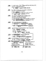
In these expressions S = Ωa y dΩa represents the first area moment of the
area Ωa with respect to the neutral axis. The resultant of these two opposite
forces – dNa – must be balanced by the longitudinal shear force dE , acting
on the contact surface between the two bodies (the squared surface). Thus,
this force takes the value ( dM = V dz , (185))
dE = Na + dNa − Na =

VS

S dM
=
dz .
I
I

(187)

If the equilibrium of the upper part were to be considered instead, an equal
force with opposite direction would be obtained, since the unbalanced force
dNa would have the opposite direction. The first area moment would be −S,
since the area moment of the whole cross-section in relation to the neutral
axis is zero. From (187) we can see that, of all possible longitudinal surfaces,
the neutral surface has the maximum longitudinal shear force, because the


254

VIII

Shear Force

maximum absolute value of the first area moment S corresponds the whole
tensioned area (or to the whole compressed area) of the cross-section.1
The longitudinal shear force per unit length is called the longitudinal shear
flow and is given by the expression
VS
dE
=
.

(188)
dz
I
In the case of inclined bending, the longitudinal shear force may be computed by superposing the forces corresponding to the decomposition of the
bending moment and the shear force in the principal axes of inertia, which
leads to the expression (cf.(150), dMx = Vy dz and dMy = −Vx dz )
f=

dE =

V y Sx
V x Sy
+
Ix
Iy

dz ,

where Sx = Ωa y dΩa and Sy = Ωa x dΩa are the first area moments of
Ωa with respect to the principal axes x and y, respectively. An alternative
expression for inclined bending is presented in Subsect. VIII.3.f.
In order to illustrate the importance of this internal force caused by the
shear force V , let us consider the cantilever beam depicted in Fig. 103, which
is made of two bars with square cross-section b × b.

P
2

b
σ

b
b

(a)

P
2

P
2

l
P
2
P
2

σ
(b)

P
2

Fig. 103. Non-uniform bending of a built-up beam: (a) without friction in the
contact surface; (b) bars perfectly connected together

If the contact surface between the two bars is lubricated, so that the friction
force between the bars is eliminated, each bar will bend independently and a
1

The same holds in the case of inclined bending, since the maximum value of dE
corresponds to the difference between the resultants of the normal stresses acting
on the whole tensioned area (or on the whole compressed area) of the cross-section.


VIII.2 The Longitudinal Shear Force

255

relative sliding in the contact surface of the bars takes place, leading to the
deformation and stress distribution represented in Fig. 103-a. The maximum
stress caused by the bending moment, which occurs in the left end crosssection, may be computed considering the force P2 acting on one beam with
square cross-section b × b, yielding
M = Mmax =

Pl
Mmax
a
⇒ σmax
= I =
2
v

Pl
2
b3
6

=3

Pl
.
b3

In the same cross-section the curvature takes the value
Pl
1
Mmax
Pl
= 2b4 = 6 4 .
=
ρa
EI
Eb
E 12

If the two bars are perfectly connected together, so that the abovementioned sliding is prevented, the two bars behave as a single unit with
a cross-section b × 2b. Thus, the deformation and the stress distribution take
the forms represented in Fig. 103-b. The maximum stress and curvature are
then given by
⎧
Mmax
Pl
3 Pl
1 a
⎪
⎪
σ b = I = b(2b)2 =
= σmax

⎪
3
⎨ max
2
b
2
v
6
M = Mmax = P l ⇒
Pl
1
M
6 Pl
1 1
⎪
max
⎪
⎪
⎩ ρ = EI = b(2b)3 = 4 Eb4 = 4 ρ .
a
E
b
12

We conclude that, by preventing the sliding in the contact surface, the
bending stiffness is multiplied by four and the loading capacity of the beam
duplicates, since the maximum stress caused by a given load P is divided by
two, i.e., twice the load may be applied for the same maximum stress. In this
case, the connection between the two bars must resist the shear flow (188)
f=

P b2 b
VS
3P
dE
=
= b(2b)23 =
.
dz
I
4 b
12

In order to see how the cross-section deforms in the presence of a shear
force, let us consider a piece with infinitesimal length dz, of a bar with a
rectangular cross-section. The bar is under non-uniform plane bending with
the action axis parallel to height h, as represented in Fig. 104. The width b of
the cross-section is very small, compared with the height h, so the shearing
stresses in the cross-section may be considered as constant and parallel to the
sides of the cross-section in the whole width.
In the horizontal surface abcd the same shearing stress τ as in the crosssection is acting, as a consequence of the reciprocity of the shearing stresses.
In this surface, the stress distribution may be admitted as uniform, since
the dimension dz is infinitesimal. The resultant of this shearing stress is the


256

VIII

Shear Force

b

h

b
a

n.a.
dE

τ

x
c

y
τ

d

V
dz

h
2

h
2

3 V

2 bh

y

Fig. 104. Shearing stresses caused by the shear force V in a rectangular cross-section
with small width

longitudinal shear force given by (187). Thus, the shearing stress takes the
value
τ b dz = dE =

V S(y)
V 1
VS
dz ⇒ τ (y) =
⇒ τ (y) =
I
Ib
I 2

h2
− y2
4

. (189)

This expression defines a parabolic stress distribution, as represented in
Fig. 104. The maximum value of the shearing stress occurs on the neutral axis
2
V

(y = 0) and takes the value τmax = V8Ih = 32 bh
.
τ
,
Since the shearing strain is proportional to the sharing stress γ = G
the cross-section must deform in such a way, that the shearing stress vanishes
in the fibres farthest from the neutral axis (y = h2 ⇒ τ = 0) and attains a
maximum value on the neutral axis (y = 0 ⇒ τ = τmax ). If the cross-section
were to remain plane, the shearing strain would be constant in the crosssection (Fig. 105-a) and the distribution of shearing stresses would not be as
represented by (189). Thus, we conclude that, either the starting hypothesis
for the analysis of the effect of the shear force is wrong (the Saint-Venant
hypothesis), or the cross-section must deform as represented in Fig. 105-b.
However, by considering all pieces of infinitesimal length dz separately,
we verify that, provided that the shear force is constant, the same warping
in all cross-sections takes place. This means that the deformations of the
different pieces are compatible, i.e., that the deformed infinitesimal pieces fit
perfectly together. Thus, no additional normal stresses are needed to make
deformations compatible, which means that the strain distribution resulting
from Saint-Venant’s hypothesis obeys all conditions of compatibility.
This example shows that the cross-section may warp without the need to
change the length of the fibres (aa = a a , Fig. 105), provided that the shear
force does not vary along the axis of the bar. Since the deformation caused by
the shear force does not require changes in the fibres’ length, this force may be
resisted without altering the distribution of the normal stresses corresponding


VIII.2 The Longitudinal Shear Force

257

γ=0
V

a

a

a
a

dz

V
π
2

(a)

− γmax
(b)

Fig. 105. Warping of a rectangular cross-section caused by the shear force V

to circular bending, i.e., there is no objection to the validity of the SaintVenant hypothesis. This conclusion may be generalized to a cross-section of
any shape, since the shearing strains corresponding to any distribution of
shearing stresses may occur without the need to change the length of the
fibres, provided that the warping is the same in all cross-sections.
These considerations are not a complete proof of the validity of the SaintVenant hypothesis in the case of constant shear force. However, they do show
that this possibility exists and the solutions of the Theory of Elasticity for particular problems confirm that, if the shear force is constant, the distribution
of normal stresses caused by the bending moment is the same as in circular

bending, i.e., it is the same as when the cross-sections remain plane and perpendicular to the bar’s axis. This means that the law of conservation of plane
sections is a sufficient condition for a linear distribution of the longitudinal
strains in the cross-section, although it may not be necessary, as we conclude
from the above considerations.
In the case of a non-constant shear force, this is no longer valid. However,
as discussed in Sect. VII.7, the error affecting the computation of the normal
stresses and, as a consequence, the computation of the longitudinal shear force
by means of (187), is very small and may even vanish (see Sect. VIII.6).
From a practical point of view, (187) may thus be considered exact. However, the computation of the shearing stress from the longitudinal shear force
always requires simplifying hypotheses, which introduce errors, whose importance depends on the shape of the cross-section. Thus, good approximations
for the shearing stress distribution are obtained for symmetrical cross-sections,
if the action axis of the shear force coincides with the symmetry axis and in the
cases of thin-walled cross-sections. In other cases it is generally not possible to
compute the shearing stresses by means of the elementary theory presented
in this book. These cases, as well as the errors introduced by the simplifying
hypotheses used are discussed below.


258

VIII

Shear Force
b

x

h

τmed

τmax

V
(a)

(b)

y

Fig. 106. Shearing stress τzy in a rectangular cross-section: (a) real distribution;
(b) admitted distribution

VIII.3 Shearing Stresses Caused by the Shear Force
VIII.3.a Rectangular Cross-Sections
In rectangular cross-sections under plane bending the simplifying hypothesis
which consists of considering the shearing strain as constant in the width of
the cross-section is usually considered: that is, the stress varies only in the
direction parallel to the action axis of the shear force. This corresponds to
the generalization to rectangular sections with any width/height ratio of the
assumptions used in previous section for the small width case. In the case of
inclined non-uniform bending, the shear force is decomposed in the symmetry
axes. Thus, in a point defined by its coordinates x and y, the two components
of the shearing stress are ((189) and Fig. 104)
⎧
2
Vy
Vy
y 2
⎪

⎨ τzy = Ix 12 h4 − y 2 = bh 32 − 6 h
(190)
⎪
⎩ τzx = Vx 1 b2 − x2 = Vx 3 − 6 x 2 .
Iy 2
4
bh 2
b
The Theory of Elasticity provides a solution for this problem, which is
obtained without the simplifying hypothesis above. This solution indicates
that the shearing stress is not constant in the direction perpendicular to the
action axis of the shear force unless the Poisson’s coefficient vanishes, but
it has a maximum in the points close to the lateral sides, as represented in
Fig. 106-a.
The maximum value of the shearing stress, which occurs for x = ± 2b and
y = 0, may be computed by the expression (cf. e.g. [4])
τmax = α

3T
2Ω

with

α=1+

ν
1+ν

h
b

2

4
2
− 2
3 π

∞
n=1,2,3,...

n2

1
cosh nπ hb

(191)
.


VIII.3 Shearing Stresses Caused by the Shear Force

259

The coefficient α represents the correction to be applied to the maximum
stress obtained from (190), in the case of plane bending, τmax = 32 VΩ . This
coefficient depends on the height/width ratio (h/b) and on the Poisson coefficient of the material, ν. The following table gives values of α, computed from
(191), for some cases.
α
h/b = 0.25

0.50
0.75
1.00
1.25
1.50
2.00
4.00

ν =0
1.0000
1.0000
1.0000
1.0000
1.0000
1.0000
1.0000
1.0000

0.05
1.2352
1.0944
1.0498
1.0301
1.0198
1.0140
1.0079
1.0020

0.1
1.4491

1.1802
1.0951
1.0574
1.0379
1.0266
1.0151
1.0038

0.15
1.6443
1.2585
1.1365
1.0823
1.0543
1.0382
1.0217
1.0054

0.2
1.8233
1.3303
1.1744
1.1052
1.0694
1.0488
1.0277
1.0069

0.25
1.9879

1.3964
1.2093
1.1263
1.0833
1.0586
1.0333
1.0083

0.3
2.1399
1.4574
1.2415
1.1457
1.0961
1.0676
1.0384
1.0096

0.4
2.4113
1.5663
1.2990
1.1804
1.1190
1.0837
1.0475
1.0119

0.5
2.6466

1.6606
1.3488
1.2104
1.1388
1.0977
1.0554
1.0139

This table shows that the error of the solution furnished by (190) increases
with the value of the Poisson coefficient and decreases as the height/width ratio increases. The dependence of the error on the relation hb has greater practical relevance, since structural materials with a Poisson coefficient smaller than
0.05 are not common, while rectangular cross-sections with height/width ratios superior to 2 are widely used.
VIII.3.b Symmetrical Cross-Sections
In practical applications cross-sections that are symmetrical with respect to
the action axis of the shear force are common. In these cases, the computation
of the shearing stresses may be carried out by considering two simplifying
hypotheses: the vertical component of the shearing stress τzy is constant in
the direction perpendicular to the symmetry axis; the total stress vectors τ in
a line perpendicular to the symmetry axis have directions converging to the
point defined by the two tangents to the cross-section’s contour on that line,
as represented in Fig. 107.
The vertical component of the shearing stress may then be computed in
the same way as in the rectangular cross-section, taking the value
τzy =

V S(y)
.
Ib(y)

(192)

The horizontal component and the resultant stress may then be obtained
from this value and angle ψ, yielding
τzx = τzy tan ψ

⇔

τ=

2 + τ2 =
τzx
zy

VS
τzy
=
.
cos ψ
Ib cos ψ

(193)


260

VIII

Shear Force

τzx
y1

x
b(y)
x

τzy

y y
2

τ

ψ
c
ψϕ
O
O
y

Fig. 107. Simplifying hypotheses for the computation of the shear force in a symmetrical cross-section

The maximum stress for a given value of y occurs clearly on the contour
S
of the cross-section, taking the value τmax = IbVcos
ϕ.
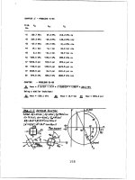
As an applied example let us consider a circular cross-section (Fig. 108).
The first area moment of the surface element defined by the central angle β
is given by the expression (Fig. 108)
dy

x

y

dS = r sin β r dβ sin β r cos β = r3 sin2 β cos β dβ .
Integrating to the whole area defined by angle α (Fig. 108), we get
α

r3 sin2 β cos β dβ =

S=
−α

2 3 3
r sin α .
3

(194)

x
r

α

β

y
y

dy

x
ϕ

b

y

Fig. 108. Computation of the shearing stress in a circular cross-section


VIII.3 Shearing Stresses Caused by the Shear Force

261

The shearing stress τzy corresponding to the area moment S (194) is then
(b = 2r sin α)
τzy (α) =

V 2 r3 sin3 α
VS
4V
4 V
= πr34
sin2 α .
sin2 α =
=
2
Ib
3
πr

3
Ω
2r
sin
α
4

For a given value α, the maximum stress occurs at the boundary. From
(193) we get
τzy
4V
τzy
=
=
sin α .
τ=
cos ϕ
sin α
3Ω
This expression attains a maximum for α = π2 (neutral axis), which means
that the maximum shear stress in the cross-section takes the value
α=

4V
π
⇒ τ = τmax =
.
2
3Ω

The solution given by the Theory of Elasticity for this problem indicates
that, unless the Poisson coefficient takes the value ν = 0.5 (incompressible
material), the stress distribution is not uniform in the neutral axis. The maximum value occurs in the centre of the circle and takes the value [4]
τmax = γ

4V
3Ω

with

γ=

9 + 6ν
.
8 (1 + ν)

The error for the approximate solution vanishes for ν = 0.5 (γ = 1) and
takes the maximum value for a vanishing Poisson’s coefficient (γ = 1.125).
For the mean value ν = 0.25, we get γ = 1.05. In the case of steel (ν = 0.3)
the error is 3.8% (γ = 1.038). We conclude that the error introduced by the
simplifying hypotheses is relatively small.
VIII.3.c Open Thin-Walled Cross-Sections
Many of the slender members currently used in structural engineering, especially in metallic constructions, have thin-walled cross-sections, i.e., cross-sections made of straight or curved elements with small thickness, in comparison
with the cross-section dimensions. Usual profile sections, such as I-beams,
channel beams, angle sections, Z-sections, T-beams, circular or rectangular
tubes, etc., are examples of this kind of member. In this Sub-section, we will
deal with open thin-walled cross-sections, i.e., simply-connected thin-walled
cross-sections.
As seen in the study of the shearing stresses in rectangular cross-sections,
if the width is small compared with the height, the simplifying hypothesis

of considering constant stresses in the thickness b is very close to the actual
distribution. The same happens in thin-walled cross-sections, like that represented in Fig. 109. Thus, by considering the longitudinal surface which is
perpendicular to the centre line of the cross-section wall and contains the


262

VIII

Shear Force

point where the shearing stress is to be computed, the shearing stress may be
obtained from the longitudinal shear force dE. From (187) we get
dE
VS
VS
⇒ τ=
=
,
(195)
I
e dz
Ie
where e represents the wall thickness in the point where τ is computed. The
computation of the area moment S of thin walls may be simplified if the area
is considered as concentrated on the centre line. Denoting by s a coordinate
which follows that line (Fig. 109), we get for the first area moment needed to
compute the shearing stress in the point defined by s2
dE = τ e dz =

M

V
M
n.a.
y

dE
s

V

s

dz

Fig. 109. Longitudinal shear force in a thin-walled cross-section

s

S (s) =

e(s )y(s ) ds .
0

In order to illustrate these considerations, the shearing stress distribution in
the cross-section represented in Fig. 110, caused by a vertical shear force V is
analysed.
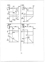
In the flange element AB the area moment corresponding to the point of
the centre line defined by the coordinate s1 may be expressed by

S(s1 ) = s1 e

h s1
+
4
2

.

The shearing stress in this point is then
τ (s1 ) =
2

V
V S(s1 )
=
Ie
I

hs1
s2
+ 1
4
2

.

If the same approximation is made for the moment of inertia, a completely
consistent theory for thin-walled cross-sections with infinitesimal wall thickness is
obtained, in the sense that the computed resultant of the shearing stress exactly

balances the applied shear force. Otherwise, a discrepancy will appear, which is
introduced by the wall curvature or by angle points in the centre line.


VIII.3 Shearing Stresses Caused by the Shear Force
s2

B
h
4

3

C

22
11

s3

s1

263

A
h

n.a.

V

× 32

h2
I

26

e
h
4

D
h
2

h
2

Fig. 110. Shearing stresses caused by a vertical positive shear force in a symmetrical
open thin-walled cross-section

The maximum stress occurs for the maximum value of s1 (point B), taking
the value
h
3 2V
AB
⇒ τ = τmax
h
.
=

s1 =
4
32 I
In the flange element BC the area moment and the shearing stress may be
expressed in terms of coordinate s2 , yielding
S (s2 ) =

V
3h2 e
h
+ s2 e ⇒ τ =
32
2
I

h
3h2
s2 +
2
32

.

In this wall segment the stress is a linear function of s2 and takes the maximum
value in point C
h
11 2 V
BC
⇒ τ = τmax
h

.
s2 =
=
2
32 I
Finally, in the web (wall segment CD) the area moment may be expressed as
a function of coordinate s3 , yielding
S(s3 ) =

22 2
h e + s3 e
32

h s3
−
2
2

⇒ τ=

V
I

22 2 s3 h s23
h +
−
32
2
2

.

This expression represents a parabolic stress distribution. The maximum value
occurs on the neutral axis and takes the value
s3 =

h
26 2 V
CD
⇒ τ = τmax
h
.
=
2
32 I

The direction of the shearing stresses may be obtained from the direction
of the longitudinal shear force. For example, in order to get the stress direction
in the flange element AB, let us consider the balance of the longitudinal forces
acting on a piece of this flange element, as represented in Fig. 111.
Let us assume a positive shear force (downward direction). As the flange
element AB is above the neutral axis, it is in the compressed zone, if the


264

VIII

Shear Force
N

N
dE

dE

τ

τ

s1
τ

τ
N + dN

dz
A

N − dN

(a)

(b)

Fig. 111. Determination of the direction of the shearing stresses in the flange
element AB (Fig. 110): (a) positive bending moment; (b) negative bending moment

bending moment is positive. A positive shear force will cause an increase in
the bending moment, as dM = V dz , which will cause an increase dN in the
compressive stress resultant N (Fig. 111-a). In the case of a negative bending

moment, the flange element AB will be in the tensioned zone. However, a
positive shear force will cause a decrease in the absolute value of the bending
moment ( dM > 0 and M < 0) and, therefore, a decrease in the tensile stress
resultant N , as represented in Fig. 111-b. In both cases, the same direction is
obtained for the shearing stress τ , as expected, since this stress is caused by
the shear force, which is the same in the two cases.
The direction of the shearing stresses in the segments BC and CD could
be obtained in the same way. The symmetry of the cross-section leads to the
directions of the shearing stresses represented in Fig. 110.
An additional tool to obtain the direction of the shearing stresses is furnished by the condition of constant shear flow in a point of convergence of two
or more centre lines of the cross-section walls, as points B and C (Fig. 110).
This condition may be obtained from the balance equation of the longitudinal
e1
dN

τ1
e2

τ2

e3

τ3

dz

dΩ

dN + ddN

Fig. 112. Shear flow in a nodal point of a thin-walled cross-section


VIII.3 Shearing Stresses Caused by the Shear Force

265

forces acting on an infinitesimal neighbourhood of one of these points (nodal
points). In the case represented in Fig. 112, this equation takes the form
infinitesimal quantity of second order

(−τ1 e1 − τ2 e2 + τ3 e3 ) dz + dσ dΩ = 0 .
infinite simal quantity of third order (ddN )

The product e dz is an infinitesimal quantity of second order, since the
thickness e is infinitesimal (cf. Footnote 55). Because dΩ is also a second
order infinitesimal quantity, dσdΩ will be an infinitesimal quantity of third
order. Thus, dσdΩ is an infinitesimal quantity of higher order, which may be
neglected, yielding
ingoing shear flow
τ1 e1 + τ2 e2 =

τ3 e3

.

(196)

outgoing shear flow
Generalizing (196) to a number n of centre lines converging to a nodal point,

we get
n

τi ei = 0 .
i=1

Taking the reciprocity of shearing stresses into consideration, this expression means that the sum of the products τ e heading into the nodal point is
equal to the sum of the products τ e heading out. In other words, the shear
flow entering the node is equal to the shear flow leaving the node. For example,
V h2 e
and the
in point C (Fig. 110) the shear flow entering the node is 2 × 11
32 I
2
22 V h e
outgoing flow is 32 I .
VIII.3.d Closed Thin-Walled Cross-Sections
If the cross-section is doubly-connected, i.e., if the centre line of the wall
is a closed line, a longitudinal cut, like the one represented in Fig. 109, is
not enough to separate the cross-section into two distinct parts. This means
that two cuts must be made and that the longitudinal shear force dE, given
by (187), is the sum of the resultants of two different longitudinal shearing
stresses, τ1 and τ2 . The value of the shearing stress cannot be computed,
therefore, unless an additional relation between τ1 and τ2 is found. However,
in the case of a symmetrical cross-section, with respect to the action axis of
the shear force, these stresses will be equal, provided that the two cuts are
made in symmetrical points of the centre line, as represented in Fig. 118. In
this case, the shearing stress may be computed by the expression
2τ e dz = dE =

VS
VS
dz ⇒ τ =
,
I
2Ie

where S is the first area moment of the shaded area in Fig. 113.

(197)


266

VIII

Shear Force

e

e
τ

τ

V

Fig. 113. Computation of the shearing stress in a closed symmetrical thin-walled
cross section

If the cross-section is not symmetrical with respect to the action axis of the
shear force, the problem becomes a statically indeterminate one, whose solution may be computed by means of the force method. As seen in Sect. VI.4, this
method consists of releasing a sufficient number of connections to get a statically determinate problem, followed by the computation of the forces needed
to avoid displacements in the released connections. In the present problem,
the longitudinal connection in a point of the cross-section wall is released, so
that an open cross-section is obtained. Under the action of the shear force, the
two sides of the cut suffer a longitudinal relative displacement, as represented
in Fig. 114-a. This displacement must then be eliminated, by applying a pair
of shear forces dE to both sides of the cut (Fig. 114-b). The resulting stress in
any point of the cross-section may be obtained by the superposition principle,
by adding the stresses corresponding to the two situations (Fig. 114-c).
B
V

V
D
B
D

τ0

A
dE

dE
τ1
A

V

V
τ0 + τ1

dz
(a)

(b)

(c)

Fig. 114. Computation of the shear stresses in a non-symmetrical closed thin-walled
cross-section


VIII.3 Shearing Stresses Caused by the Shear Force

267

The relative displacement in direction z of two points of the centre line,
located at an infinitesimal distance ds of each other, is dD = γ0 ds .3 Thus, in
the open cross-section, the relative displacement D of both sides of the cut,
caused by the shear force V (Fig. 114-a), may be computed by integrating
the shear strain γ0 along the complete centre line of the wall, which yields
(τ0 = Gγ0 )
1
V
S
ds .
(198)
D = γ0 ds =

τ0 ds =
G
IG
e
In the situation depicted in Fig. 114-b, the shear flow f = τ1 (s)e(s) is
constant along the whole centre line of the wall,4 since there are no other
forces applied to the bar apart from the pair of forces dE . This conclusion is
easily drawn by establishing the balance condition of the longitudinal forces
acting on the piece defined by the longitudinal cut AA and by any other
longitudinal surface BB (Fig. 114-b). This condition immediately means that
the product τ1 e = dE
dz = f is constant, even if e varies along the centre line.
The longitudinal relative displacement D caused by the pair of forces dE , is
then (τ1 = fe )
f
τ1
ds
ds =
.
(199)
D = γ1 ds =
G
G
e
The condition of compatibility requires that the displacement D eliminates
displacement D, which allows the computation of the shear flow f
D+D =0 ⇒ f =−

V
I

S
e ds
ds
e

⇒ τ1 (s) =

f
.
e(s)

(200)

The shearing stress in the closed cross-section (Fig. 114-c) may then be computed by adding the stresses τ0 and τ1 .
The closed line integrals appearing in the expressions above obviously refer
to the line limiting the closed part of the cross-section, that is, they do not
include simply-connected walls, as in the cross-section represented in Fig. 115.
The expressions above are valid for doubly-connected cross-sections, i.e.,
closed cross-sections with only one channel. In cross-sections with higher degrees of connection a number of longitudinal cuts equal to the degree of connection minus one is necessary to get a statically determinate problem, i.e.,
an open cross-section. As a consequence, the conditions of compatibility of
the deformations in all the longitudinal cuts yield, instead of (200), a system
3

This simple relation requires that the fibres remain parallel to each other in
the deformation caused by the shear force. This condition is satisfied if there is no
rotation of the cross-sections around a longitudinal axis of the prismatic bar, i.e., if
torsion does not take place (see example XII.8).
4
This shear flow defines a torsional moment (twisting moment or torque, see

Chap. X.3). This moment corresponds to the translation of the shear force, from the
shear centre of the open cross-section to the shear centre of the closed cross-section
(see Sect. VIII.4 and example VIII.12).


268

VIII

Shear Force

V

Fig. 115. Line, to which the closed line integrals in (198), (199) and (200) are
referred (dashed line)

with a number of equations equal to the degree of connection minus one (see
example VIII.7).
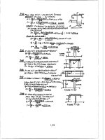
VIII.3.e Composite Members
In composite members the longitudinal shear force may be determined in the
same way as in the case of homogeneous bars (187). The normal stress is in
this case given by (169). Assuming, for simplicity, plane bending, as in the case
represented in Fig. 116, we get the following expression for the longitudinal
shear force (Fig. 116-b)
⎧
dM Ea
⎪
⎪
y
dE = Ωa1 dσa dΩa + Ωb1 dσb dΩb

⎨ dσa = J
n
⇒
⎪
dM Eb
⎪
= JVn Ea Ωa1y dΩa + Eb Ωb1y dΩb dz .
⎩ dσb =
y
Jn
(201)

Ωa

n.a.

n.a.
Ωa1

Ωb
Ωb1
V
(a)

V
(b)

Fig. 116. Determination of the longitudinal shear force in composite members

VIII.3 Shearing Stresses Caused by the Shear Force

269

In composite members, the longitudinal shear force in the contact surface
between the two materials must usually be computed. In this particular case
(201) takes a simpler form and the longitudinal shear force may be computed
by any of the following expressions
⎧
Ωa1 = Ωa
⎪
⎪
⎪
⎪
V E a Sa
dE
V Sa
⎪
⎪
=
⇒
=
with Sa =
y dΩa
⎪
⎪
dz
J
Iha
⎪

n
Ωa
⎪
⎪
⎪ Ωb1 = 0
⎨
(202)
⎪
⎪
=
0
Ω
⎪
a1
⎪
⎪
⎪
V E b Sb
V Sb
dE
⎪
⎪
=
=
with Sb =
y dΩb .
⇒
⎪
⎪
dz

J
Ihb
⎪
n
Ωb
⎪
⎩
Ωb1 = Ωb
VIII.3.f Non-Principal Reference Axes
In some cross-sections it is easy to compute the moments and product of
inertia with respect to non-principal central axes, as well as distances and
area moments. In Fig. 117 two examples of this kind of cross-section are
represented.
In these cases it may be useful to compute the normal and shearing stresses
directly from these axes, especially if one of them is parallel to the action axis.
The normal stresses may by computed by means of (140). From this equation an expression for the computation of the longitudinal shear force may
then be developed. If the bending moment has only the Mx component and
the axial force vanishes, the normal stress may be computed by the expression
σ=

Iy y − Ixy x
Mx .
2
Ix Iy − Ixy

The same line of reasoning used to develop (186), leads to the following
expression for the longitudinal shear force (cf. Figs. 102 and 117)

x

Mx

x

Mx

Ωa

Ωa
y

y

Fig. 117. Computation of the longitudinal shear force with non-principal reference
axes


270

VIII

Shear Force

dE =
Ωa

Iy y − Ixy x
Iy Sx − Ixy Sy
dMx dΩa = Vy
dz

2
2
Ix Iy − Ixy
Ix Iy − Ixy

dMx
,
with Vy =
dz

Sx =

y dΩa
Ωa

and Sy =

(203)

x dΩa .
Ωa

The shearing stresses may be computed from this expression, in the same way
as was done on the basis of (187) (see example VIII.10).

VIII.4 The Shear Centre
When inclined circular bending was analysed (Sect. VII.4), we showed that a
parallel displacement of the action axis does not change the normal stresses
induced by the bending moment in the cross-section. However, if a shear
force is acting (non-uniform bending), the equilibrium condition requires that

the action axis of the shear force has a position which coincides with the
line of action of the resultant of the shearing stresses. The position of the
action axis of the shear force is therefore not arbitrary. There are two internal
forces introducing shearing stresses in the cross-section: the shear force and
the torsional moment. The expressions presented for the shearing stresses in
this Chapter only take the shear force into consideration, since they are all
based on the relation dM = V dz (185). It is therefore assumed that the
torsional moment is zero. If it is not, additional shearing stresses will appear.
These stresses will be analysed in Chap. X.
Thus, to avoid torsion, the action axis of the shear stress must coincide with
the line of action of the resultant of the shearing stresses computed by means
of the expressions which were developed from (187) (longitudinal shear force
caused by the cross-sectional shear force). By considering two shear forces
with the directions of the principal central axes of inertia, and computing the
position of the line of action of the resultant of the shearing stresses in each
case, a point is defined by the intersection of these two lines, which has the
following property: if the line of action of the shear force passes through this
point, it will not induce torsion of the bar. This point is the shear centre of
the cross-section.
The shear centre plays the same role in relation to the transversal forces,
as the centroid in relation to the longitudinal (axial) forces: if the resultant
axial force passes through the centroid of the cross-section, it will not induce
bending; otherwise, composed bending will take place, with a bending moment
given by the product of the axial force and the distance of its line of action
to the centroid. In the same way, if the resultant of the forces acting on the
cross-section plane (the shear force) does not pass through the shear centre,
it will introduce a torsional moment, with a value given by the product of the
shear force and the distance of its line of action to the shear centre.
The computation of the torsional moment must thus be made in relation
to the shear centre, while the bending moment is computed with respect to the

VIII.4 The Shear Centre

271

centroid. In the case of a cross-section with a symmetry axis, the shear centre
is on this axis, since, for an action axis of the shear force coinciding with the
symmetry axis, the shearing stress distribution will also be symmetric, which
means that the line of action of its resultant coincides with the symmetry axis.
Thus, if the cross-section has two symmetry axes the centroid and the shear
centre will coincide. In other cases, these two points usually occupy different
positions in the cross-section’s plane.
We will demonstrate later (Chap. XII) that in prismatic bars made of
materials with linear elastic behaviour, the shear centre coincides with the
torsion centre, which is defined as the point around which the cross-section
rotates in the twisting deformation induced by the torsional moment. For this
reason, these two designations are sometimes indistinctly used.
While it is very easy to compute the position of the line of action of the resultant of the normal stresses in the case of pure axial force, since these stresses
are constant in the cross-section, the computation of the line of action of the
resultant of the shearing stresses is often complex, since the distribution of
the stresses caused by the shear force is required. As seen in the previous sections, good approximations for these stresses are obtained only in the cases of
symmetrical cross-sections with respect to the action axis of the shear force
and in thin-walled cross-sections. In the first case, the position of the resultant
is known. In the case of non-symmetrical cross-sections which cannot be considered as thin-walled, the problem of computing the shear centre’s position
cannot be solved by the approach used in the Strength of Materials. But the
knowledge of the position of the shear centre is most important in the case of
open thin walled cross-sections, since this kind of member is very weak in torsion, as will be seen in Chap. X. Fortunately, the stresses caused by the shear
force in these cross-sections are easily computed with good approximation, as
seen in Subsect. VIII.3.c.

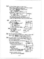
In order to illustrate these considerations, the position of the shear centre
of the channel cross-section represented in Fig. 118 is computed. As this crosssection has a symmetry axis, the shear centre will be located on this axis.
Rb

B
A
e

h

V bh
I 2

d

C
V
I

h2
8

E
D

D

b
(a)

Ra

(b)

Ra
Rb
(c)

Fig. 118. Computation of the position of the shear centre in a thin-walled crosssection


272

VIII

Shear Force

Thus, in order to determine its position, it is enough to compute the distance
d from the line of action of the resultant of the shearing stresses, introduced
by a shear force perpendicular to the symmetry axis, to the centre line of the
web (Fig. 118-c).
As the example of (Fig. 110) shows, the shearing stress has a linear distribution in the wall segments which are parallel to the neutral axis, and
a parabolic distribution in the others. Besides, we know that the maximum
stress occurs on the neutral axis. For these reasons, in example of (Fig. 118)
the stress distribution is completely defined by the values in points B and C.
For point B we get from (195)
S = be

V bh
h

⇒ τ=
.
2
I 2

For point C the same expression yields the value
S=

bh h2
+
2
8

V
beh h h
+ e ⇒ τ=
2
2 4
I

.

The resultants of the shearing stress in the web (Ra ) and in the flanges (Rb )
may be computed from the diagram areas in Fig. 118-b, multiplied by the
thickness e, yielding
Ra =

V
I

bh
2 h2
he +
he
2
3 8

=

V
I

eh3
+ 2 × be
12
Ia

2

Rb

V b he
1 V bh
be =
≈
2I 2
I 4

3
h 2

b

+ 6 hb

2

h
2

≈V
3

Ib − be
12

(204)

V .

It must be remarked here that, as mentioned in Footnote 55, an exact
balance between the shear force and the resultant of the shearing stresses is
only achieved if the moment of inertia of the flange, with respect to is centre
3
5
line ( be
12 ), is neglected. The condition of equivalence of moments with respect
to point D (Fig. 118-c) allows the computation of the distance d, which defines
the position of the shear centre
Rb h = Ra d ⇒ d =

5

3
h 2
b

+ 6 hb

h.

(205)

From a mathematical point of view, the theory expounded for thin-walled crosssections is only valid if the thickness of the walls is infinitesimal, in comparison with
the cross-section dimensions. In this case, the moment of inertia of the flange with
3
, is an infinitesimal quantity of third order, which may
respect to its centre line, be
12
be neglected in presence of the infinitesimal quantity of first order resulting from
2
.
the parallel-axis theorem, beh
4


VIII.5 Non-Prismatic Members

273

Fig. 119. Shear centre in thin-walled cross-sections with concurrent and straight

wall elements

The thin-walled cross-sections with concurrent and straight wall elements,
like those represented in Fig. 119, are a particularly simple case of determination of the shear centre. In fact, as the resultants of the shearing stresses in
the different wall elements pass through the intersection of the centre lines,
the moment of the shearing stress in relation to this point vanishes, which
means that it is the shear centre.

VIII.5 Non-Prismatic Members
VIII.5.a Introduction
The basic equation for the analysis of the effect of the shear force (187) has
been deduced for prismatic bars. So when the above expressions for the computation of shearing stresses are applied to non-prismatic members, errors
are introduced. In order to get an idea of the importance of these errors, two
examples of non-prismatic members, which are simple enough for an exact
solution to be given by the Theory of Elasticity, are analysed.
VIII.5.b Slender Members with Curved Axis
As explained in Sect. VIII.2, the expression obtained for the shearing stress
in a rectangular cross-section with a small thickness (189) coincides with the
exact solution of the Theory of Elasticity. Thus, in a bar with the same crosssection, but with a curved axis, the discrepancies between the exact solution
and the results obtained using (187) may be attributed to the fact that the
bar’s axis is not a straight line.
The bar represented in Fig. 120 has a circular axis and a rectangular crosssection with the dimensions b × h (b
h). The shear force in the cross-section
B defined by the angle θ takes the value V = −P cos θ.
The shearing stress in that cross-section may be expressed as a function of
the dimensionless coordinate η, which, multiplied by the height of the crosssection h, defines the distance to the centre line (− 12 ≤ η ≤ 12 , Fig. 120). The
exact solution obtained by the Theory of Elasticity for the shearing stress on
the cross-section defined by the angle θ may be defined by the expression [4]

274

VIII

Shear Force

h P
B
θ

rm

C
ηh

η0 h
τmax

Fig. 120. Shearing stresses induced by the shear force in a bar with a curved axis
1− α

2

2

2 1+ α

2

4

4
3 P cos θ 1 + ηα + (1+ηα)3 − 1+ηα
τ =−
2
2+α
2 bh
3 − α3 1 + α4 ln 2−α

with α =

h
.
rm

(206)

γ

In the limit case of a prismatic bar (α = 0, θ = π) this solution yields the
V
same value as (190) τmax = 32 bh
.
When the relation α between the height of the cross-section and the curvature radius of the centre line rm increases, the difference between the distributions of shearing stresses given by (206) and by the expression developed
for prismatic bars increases also. This difference remains small, however, even
for larger curvatures, as may be easily confirmed by computing the values of
η and γ corresponding to the maximum shearing stress (η = η0 ⇒ γ = γmax )
for some values of α
α
0.0000 0.1000 0.2500 0.5000 0.7500 1.0000 1.5000
η0

0.0000 0.0250 0.0626 0.1259 0.1905 0.2565 0.3885
γmax 1.0000 1.0009 1.0056 1.0233 1.0573 1.1166 1.4402

VIII.5.c Slender Members with Variable Cross-Section
In bars with variable cross-section the expressions developed on the basis of
(187) may lead to completely erroneous results, at least in relation to the location of the maximum stress in the cross-section. For example, in the problem
represented in Fig. 86, the exact solution shows that the shearing stress vanishes in the neutral axis and attains the maximum value in the farthest points


VIII.6 Influence of a Non-Constant Shear Force

275

from the neutral axis, as may be easily ascertained by a two-dimensional analysis of the stress state in those points, which totally contradicts the solution
developed for prismatic bars.
Regarding the value of the maximum shearing stress in the cross-section,
significant errors may also be introduced by the theory of prismatic bars, as
may be easily verified by computing the maximum shearing stress in crosssection AA (Fig. 86). From (164) we find that the maximum radial stress
occurs in point A and takes the value
ϕ=

α
P
α
2
⇒ σr = σr−max =
sin .
2
α − sin α br
2

A two-dimensional analysis of the stress state shows that the shearing
stress in a vertical facet takes the value
τmax =

2 sin2 α2 cos α2 P
α
1
α
σr−max sin α = sin cos σr−max =
.
2
2
2
α − sin α br

The theory of prismatic bars yields the following value for the maximum
shearing stress in the same cross-section, τmax−p
⎧
h = 2r sin α2
⎪
⎪
⎨
3 1 P
3V
=
.
⇒ τmax−p =
2 bh
4 sin α2 br

⎪
⎪
⎩
V =P
The relation between the exact value τmax and the value yield by the
theory of prismatic bars, τmax−p , depends only on angle α and may expressed
by parameter β
8 sin3 α2 cos α2
τmax
.
=
β=
τmax−p
3 α − sin α
The following Table gives the values of β corresponding to some values of
angle α.
α 1◦
10◦ 20◦ 30◦ 45◦ 60◦
β 1.999 1.988 1.952 1.892 1.764 1.593

This example shows that the actual value of the maximum shearing stress
in a slender member with a variable cross-section may be substantially higher
than the value given by the theory of prismatic bars.

VIII.6 Influence of a Non-Constant Shear Force
The solution of the Theory of Elasticity for the shearing stresses in the example depicted in Fig. 85 (162) shows that (189) is exact (V = p 2l − z ),