Ebook Number theory - An introduction to mathematics (2/E): Part 2

VII
The Arithmetic of Quadratic Forms

We have already determined the integers which can be represented as a sum of
two squares. Similarly, one may ask which integers can be represented in the form
x 2 + 2y 2 or, more generally, in the form ax 2 + 2bx y + cy 2 , where a, b, c are given
integers. The arithmetic theory of binary quadratic forms, which had its origins in
the work of Fermat, was extensively developed during the 18th century by Euler,
Lagrange, Legendre and Gauss. The extension to quadratic forms in more than two
variables, which was begun by them and is exemplified by Lagrange’s theorem that
every positive integer is a sum of four squares, was continued during the 19th century by Dirichlet, Hermite, H.J.S. Smith, Minkowski and others. In the 20th century
Hasse and Siegel made notable contributions. With Hasse’s work especially it became apparent that the theory is more perspicuous if one allows the variables to be
rational numbers, rather than integers. This opened the way to the study of quadratic
forms over arbitrary fields, with pioneering contributions by Witt (1937) and Pfister
(1965–67).
From this vast theory we focus attention on one central result, the Hasse–Minkowski
theorem. However, we first study quadratic forms over an arbitrary field in the geometric formulation of Witt. Then, following an interesting approach due to Fr¨ohlich
(1967), we study quadratic forms over a Hilbert field.

1 Quadratic Spaces
The theory of quadratic spaces is simply another name for the theory of quadratic
forms. The advantage of the change in terminology lies in its appeal to geometric
intuition. It has in fact led to new results even at quite an elementary level. The new
approach had its debut in a paper by Witt (1937) on the arithmetic theory of quadratic
forms, but it is appropriate also if one is interested in quadratic forms over the real field
or any other field.
For the remainder of this chapter we will restrict attention to fields for which
1 + 1 = 0. Thus the phrase ‘an arbitrary field’ will mean ‘an arbitrary field of characteristic = 2’. The proofs of many results make essential use of this restriction on the
W.A. Coppel, Number Theory: An Introduction to Mathematics, Universitext,
DOI: 10.1007/978-0-387-89486-7_7, © Springer Science + Business Media, LLC 2009

291


292

VII The Arithmetic of Quadratic Forms

characteristic. For any field F, we will denote by F × the multiplicative group of all
nonzero elements of F. The squares in F × form a subgroup F ×2 and any coset of this
subgroup is called a square class.
Let V be a finite-dimensional vector space over such a field F. We say that V is a
quadratic space if with each ordered pair u, v of elements of V there is associated an
element (u, v) of F such that
(i) (u 1 + u 2 , v) = (u 1 , v) + (u 2 , v) for all u 1 , u 2 , v ∈ V ;
(ii) (αu, v) = α(u, v) for every α ∈ F and all u, v ∈ V ;
(iii) (u, v) = (v, u) for all u, v ∈ V .
It follows that
(i) (u, v 1 + v 2 ) = (u, v 1 ) + (u, v 2 ) for all u, v 1 , v 2 ∈ V ;
(ii) (u, αv) = α(u, v) for every α ∈ F and all u, v ∈ V .
Let e1 , . . . , en be a basis for the vector space V . Then any u, v ∈ V can be uniquely
expressed in the form
n

n

u=

ξjej,

v=

j =1

ηjej,
j =1

where ξ j , η j ∈ F( j = 1, . . . , n), and
n

α j k ξ j ηk ,

(u, v) =
j,k=1

where α j k = (e j , ek ) = αkj . Thus
n

α j k ξ j ξk

(u, u) =
j,k=1

is a quadratic form with coefficients in F. The quadratic space is completely determined by the quadratic form, since
(u, v) = {(u + v, u + v) − (u, u) − (v, v)}/2.

(1)

Conversely, for a given basis e1 , . . . , en of V , any n × n symmetric matrix
A = (α j k ) with elements from F, or the associated quadratic form f (x) = x t Ax,
may be used in this way to give V the structure of a quadratic space.

Let e1 , . . . , en be any other basis for V . Then
n

ei =

τ jie j ,
j =1

where T = (τi j ) is an invertible n × n matrix with elements from F. Conversely, any
such matrix T defines in this way a new basis e1 , . . . , en . Since


1 Quadratic Spaces

293

n

(ei , ek ) =

τ j i β j h τhk ,
j,h=1

where β j h = (e j , eh ), the matrix B = (β j h ) is symmetric and
A = T t BT.

(2)

Two symmetric matrices A, B with elements from F are said to be congruent if (2)
holds for some invertible matrix T with elements from F. Thus congruence of symmetric matrices corresponds to a change of basis in the quadratic space. Evidently

congruence is an equivalence relation, i.e. it is reflexive, symmetric and transitive. Two
quadratic forms are said to be equivalent over F if their coefficient matrices are congruent. Equivalence over F of the quadratic forms f and g will be denoted by f ∼ F g
or simply f ∼ g.
It follows from (2) that
det A = (det T )2 det B.
Thus, although det A is not uniquely determined by the quadratic space, if it is nonzero,
its square class is uniquely determined. By abuse of language, we will call any representative of this square class the determinant of the quadratic space V and denote it by
det V .
Although quadratic spaces are better adapted for proving theorems, quadratic
forms and symmetric matrices are useful for computational purposes. Thus a familiarity with both languages is desirable. However, we do not feel obliged to give two
versions of each definition or result, and a version in one language may later be used
in the other without explicit comment.
A vector v is said to be orthogonal to a vector u if (u, v) = 0. Then also u is
orthogonal to v. The orthogonal complement U ⊥ of a subspace U of V is defined to
be the set of all v ∈ V such that (u, v) = 0 for every u ∈ U . Evidently U ⊥ is again a
subspace. A subspace U will be said to be non-singular if U ∩ U ⊥ = {0}.
The whole space V is itself non-singular if and only if V ⊥ = {0}. Thus V is
non-singular if and only if some, and hence every, symmetric matrix describing it is
non-singular, i.e. if and only if det V = 0.
We say that a quadratic space V is the orthogonal sum of two subspaces V1 and
V2 , and we write V = V1 ⊥V2 , if V = V1 + V2 , V1 ∩ V2 = {0} and (v 1 , v 2 ) = 0 for all
v 1 ∈ V1 , v 2 ∈ V2 .
If A1 is a coefficient matrix for V1 and A2 a coefficient matrix for V2 , then
A=

A1
0

0
A2

is a coefficient matrix for V = V1 ⊥V2 . Thus det V = (det V1 )(det V2 ). Evidently V is
non-singular if and only if both V1 and V2 are non-singular.
If W is any subspace supplementary to the orthogonal complement V ⊥ of the
whole space V , then V = V ⊥ ⊥W and W is non-singular. Many problems for arbitrary
quadratic spaces may be reduced in this way to non-singular quadratic spaces.


294

VII The Arithmetic of Quadratic Forms

Proposition 1 If a quadratic space V contains a vector u such that (u, u) = 0, then
V = U ⊥U ⊥ ,
where U = u is the one-dimensional subspace spanned by u.
Proof For any vector v ∈ V , put v = v − αu, where α = (v, u)/(u, u). Then (v , u) =
0 and hence v ∈ U ⊥ . Since U ∩ U ⊥ = {0}, the result follows.
✷
A vector space basis u 1 , . . . , u n of a quadratic space V is said to be an orthogonal
basis if (u j , u k ) = 0 whenever j = k.
Proposition 2 Any quadratic space V has an orthogonal basis.
Proof If V has dimension 1, there is nothing to prove. Suppose V has dimension
n > 1 and the result holds for quadratic spaces of lower dimension. If (v, v) = 0 for
all v ∈ V , then any basis is an orthogonal basis, by (1). Hence we may assume that
V contains a vector u 1 such that (u 1 , u 1 ) = 0. If U1 is the 1-dimensional subspace
spanned by u 1 then, by Proposition 1,
V = U1 ⊥U1⊥ .
By the induction hypothesis U1⊥ has an orthogonal basis u 2 , . . . , u n , and u 1 , u 2 , . . . , u n
is then an orthogonal basis for V .
✷

Proposition 2 says that any symmetic matrix A is congruent to a diagonal matrix,
or that the corresponding quadratic form f is equivalent over F to a diagonal form
δ1 ξ12 + · · · + δn ξn2 . Evidently det f = δ1 · · · δn and f is non-singular if and only if
δ j = 0 (1 ≤ j ≤ n). If A = 0 then, by Propositions 1 and 2, we can take δ1 to be any
element of F × which is represented by f .
Here γ ∈ F × is said to be represented by a quadratic space V over the field F if
there exists a vector v ∈ V such that (v, v) = γ .
As an application of Proposition 2 we prove
Proposition 3 If U is a non-singular subspace of the quadratic space V , then
V = U ⊥U ⊥ .
Proof Let u 1 , . . . , u m be an orthogonal basis for U . Then (u j , u j ) = 0 (1 ≤ j ≤ m),
since U is non-singular. For any vector v ∈ V , let u = α1 u 1 + · · · + αm u m , where
α j = (v, u j )/(u j , u j ) for each j . Then u ∈ U and (u, u j ) = (v, u j ) (1 ≤ j ≤ m).
Hence v − u ∈ U ⊥ . Since U ∩ U ⊥ = {0}, the result follows.
✷
It may be noted that if U is a non-singular subspace and V = U ⊥W for some
subspace W , then necessarily W = U ⊥ . For it is obvious that W ⊆ U ⊥ and
dim W = dim V − dim U = dim U ⊥ , by Proposition 3.
Proposition 4 Let V be a non-singular quadratic space. If v 1 , . . . , v m are linearly
independent vectors in V then, for any η1 , . . . , ηm ∈ F, there exists a vector v ∈ V
such that (v j , v) = η j (1 ≤ j ≤ m).
Moreover, if U is any subspace of V , then


1 Quadratic Spaces

295

(i) dim U + dim U ⊥ = dim V ;
(ii) U ⊥⊥ = U ;

(iii) U ⊥ is non-singular if and only if U is non-singular.
Proof There exist vectors v m+1 , . . . , v n ∈ V such that v 1 , . . . , v n form a basis for V .
If we put α j k = (v j , v k ) then, since V is non-singular, the n × n symmetric matrix
A = (α j k ) is non-singular. Hence, for any η1 , . . . , ηn ∈ F, there exist unique
ξ1 , . . . , ξn ∈ F such that v = ξ1 v 1 + · · · + ξn v n satisfies
(v 1 , v) = η1 , . . . , (v n , v) = ηn .
This proves the first part of the proposition.
By taking U = v 1 , . . . , v m and η1 = · · · = ηm = 0, we see that dim U ⊥ = n−m.
Replacing U by U ⊥ , we obtain dim U ⊥⊥ = dim U . Since it is obvious that U ⊆ U ⊥⊥ ,
this implies U = U ⊥⊥ . Since U non-singular means U ∩ U ⊥ = {0}, (iii) follows at
once from (ii).
✷
We now introduce some further definitions. A vector u is said to be isotropic if
u = 0 and (u, u) = 0. A subspace U of V is said to be isotropic if it contains an
isotropic vector and anisotropic otherwise. A subspace U of V is said to be totally
isotropic if every nonzero vector in U is isotropic, i.e. if U ⊆ U ⊥ . According to these
definitions, the trivial subspace {0} is both anisotropic and totally isotropic.
A quadratic space V over a field F is said to be universal if it represents every
γ ∈ F × , i.e. if for each γ ∈ F × there is a vector v ∈ V such that (v, v) = γ .
Proposition 5 If a non-singular quadratic space V is isotropic, then it is universal.
Proof Since V is isotropic, it contains a vector u = 0 such that (u, u) = 0. Since
V is non-singular, it contains a vector w such that (u, w) = 0. Then w is linearly
independent of u and by replacing w by a scalar multiple we may assume (u, w) = 1.
If v = αu + w, then (v, v) = γ for α = {γ − (w, w)}/2.
✷
On the other hand, a non-singular universal quadratic space need not be isotropic.
As an example, take F to be the finite field with three elements and V the
2-dimensional quadratic space corresponding to the quadratic form ξ12 + ξ22 .
Proposition 6 A non-singular quadratic form f (ξ1 , . . . , ξn ) with coefficients from a
field F represents γ ∈ F × if and only if the quadratic form

g(ξ0 , ξ1 , . . . , ξn ) = −γ ξ02 + f (ξ1 , . . . , ξn )
is isotropic.
Proof Obviously if f (x 1 , . . . , x n ) = γ and x 0 = 1, then g(x 0 , x 1 , . . . , x n ) = 0.
Suppose on the other hand that g(x 0, x 1 , . . . , x n ) = 0 for some x j ∈ F, not all zero.
If x 0 = 0, then f certainly represents γ . If x 0 = 0, then f is isotropic and hence, by
Proposition 5, it still represents γ .
✷
Proposition 7 Let V be a non-singular isotropic quadratic space. If V = U ⊥W , then
there exists γ ∈ F × such that, for some u ∈ U and w ∈ W ,
(u, u) = γ ,

(w, w) = −γ .


296

VII The Arithmetic of Quadratic Forms

Proof Since V is non-singular, so also are U and W , and since V contains an isotropic
vector v , there exist u ∈ U , w ∈ W , not both zero, such that
(u , u ) = −(w , w ).
If this common value is nonzero, we are finished. Otherwise either U or W is
isotropic. Without loss of generality, suppose U is isotropic. Since W is non-singular,
it contains a vector w such that (w, w) = 0, and U contains a vector u such that
(u, u) = −(w, w), by Proposition 5.
✷
We now show that the totally isotropic subspaces of a quadratic space are important for an understanding of its structure, even though they are themselves trivial as
quadratic spaces.
Proposition 8 All maximal totally isotropic subspaces of a quadratic space have the
same dimension.

Proof Let U1 be a maximal totally isotropic subspace of the quadratic space V . Then
U1 ⊆ U1⊥ and U1⊥ \U1 contains no isotropic vector. Since V ⊥ ⊆ U1⊥ , it follows that
V ⊥ ⊆ U1 . If V is a subspace of V supplementary to V ⊥ , then V is non-singular
and U1 = V ⊥ + U1 , where U1 ⊆ V . Since U1 is a maximal totally isotropic subspace
of V , this shows that it is sufficient to establish the result when V itself is non-singular.
Let U2 be another maximal totally isotropic subspace of V . Put W = U1 ∩ U2 and
let W1 , W2 be subspaces supplementary to W in U1 , U2 respectively. We are going to
show that W2 ∩ W1⊥ = {0}.
Let v ∈ W2 ∩ W1⊥ . Since W2 ⊆ U2 , v is isotropic and v ∈ U2⊥ ⊆ W ⊥ . Hence
v ∈ U1⊥ and actually v ∈ U1 , since v is isotropic. Since W2 ⊆ U2 this implies v ∈ W ,
and since W ∩ W2 = {0} this implies v = 0.
It follows that dim W2 + dim W1⊥ ≤ dim V . But, since V is now assumed nonsingular, dim W1 = dim V − dim W1⊥ , by Proposition 4. Hence dim W2 ≤ dim W1
and, for the same reason, dim W1 ≤ dim W2 . Thus dim W2 = dim W1 , and hence
dim U2 = dim U1 .
✷
We define the index, ind V , of a quadratic space V to be the dimension of any
maximal totally isotropic subspace. Thus V is anisotropic if and only if ind V = 0.
A field F is said to be ordered if it contains a subset P of positive elements, which
is closed under addition and multiplication, such that F is the disjoint union of the sets
{0}, P and −P = {−x : x ∈ P}. The rational field Q and the real field R are ordered
fields, with the usual interpretation of ‘positive’. For quadratic spaces over an ordered
field there are other useful notions of index.
A subspace U of a quadratic space V over an ordered field F is said to be
positive definite if (u, u) > 0 for all nonzero u ∈ U and negative definite if (u, u) < 0
for all nonzero u ∈ U . Evidently positive definite and negative definite subspaces are
anisotropic.
Proposition 9 All maximal positive definite subspaces of a quadratic space V over an
ordered field F have the same dimension.

1 Quadratic Spaces

297

Proof Let U+ be a maximal positive definite subspace of the quadratic space V . Since
U+ is certainly non-singular, we have V = U+ ⊥W , where W = U+⊥ , and since U+ is
maximal, (w, w) ≤ 0 for all w ∈ W . Since U+ ⊆ V , we have V ⊥ ⊆ W . If U− is a
maximal negative definite subspace of W , then in the same way W = U− ⊥U0 , where
U0 = U−⊥ ∩ W . Evidently U0 is totally isotropic and U0 ⊆ V ⊥ . In fact U0 = V ⊥ ,
since U− ∩ V ⊥ = {0}. Since (v, v) ≥ 0 for all v ∈ U+ ⊥V ⊥ , it follows that U− is a
maximal negative definite subspace of V .
If U+ is another maximal positive definite subspace of V , then U+ ∩ W = {0} and
hence
dim U+ + dim W = dim(U+ + W ) ≤ dim V .
Thus dim U+ ≤ dim V − dim W = dim U+ . But U+ and U+ can be interchanged. ✷
If V is a quadratic space over an ordered field F, we define the positive index
ind+ V to be the dimension of any maximal positive definite subspace. Similarly all
maximal negative definite subspaces have the same dimension, which we will call the
negative index of V and denote by ind− V . The proof of Proposition 9 shows that
ind+ V + ind− V + dim V ⊥ = dim V.
Proposition 10 Let F denote the real field R or, more generally, an ordered field in
which every positive element is a square. Then any non-singular quadratic form f in
n variables with coefficients from F is equivalent over F to a quadratic form
2
g = ξ12 + · · · + ξ p2 − ξ p+1
− · · · − ξn2 ,

where p ∈ {0, 1, . . . , n} is uniquely determined by f . In fact,
ind+ f = p, ind− f = n − p, ind f = min( p, n − p).
Proof By Proposition 2, f is equivalent over F to a diagonal form δ1 η12 + · · · + δn ηn2 ,

where δ j = 0 (1 ≤ j ≤ n). We may choose the notation so that δ j > 0 for j ≤ p and
1/2
δ j < 0 for j > p. The change of variables ξ j = δ j η j ( j ≤ p), ξ j = (−δ j )1/2 η j
( j > p) now brings f to the form g. Since the corresponding quadratic space has a
p-dimensional maximal positive definite subspace, p = ind+ f is uniquely determined. Similarly n − p = ind− f , and the formula for ind f follows readily.
✷
It follows that, for quadratic spaces over a field of the type considered in Proposition 10, a subspace is anisotropic if and only if it is either positive definite or negative
definite.
Proposition 10 completely solves the problem of equivalence for real quadratic
forms. (The uniqueness of p is known as Sylvester’s law of inertia.) It will now be
shown that the problem of equivalence for quadratic forms over a finite field can also
be completely solved.
Lemma 11 If V is a non-singular 2-dimensional quadratic space over a finite field
Fq , of (odd) cardinality q, then V is universal.


298

VII The Arithmetic of Quadratic Forms

Proof By choosing an orthogonal basis for V we are reduced to showing that if α, β,
2
2
γ ∈ F×
q , then there exist ξ, η ∈ Fq such that αξ + βη = γ . As ξ runs through Fq ,
αξ 2 takes (q + 1)/2 = 1 + (q − 1)/2 distinct values. Similarly, as η runs through Fq ,
γ − βη2 takes (q + 1)/2 distinct values. Since (q + 1)/2 + (q + 1)/2 > q, there exist
ξ, η ∈ Fq for which αξ 2 and γ − βη2 take the same value.
✷
Proposition 12 Any non-singular quadratic form f in n variables over a finite field Fq

is equivalent over Fq to the quadratic form
2
+ δξn2 ,
ξ12 + · · · + ξn−1

where δ = det f is the determinant of f .
There are exactly two equivalence classes of non-singular quadratic forms in n
variables over Fq , one consisting of those forms f whose determinant det f is a square
×
in F×
q , and the other those for which det f is not a square in Fq .
Proof Since the first statement of the proposition is trivial for n = 1, we assume that
n > 1 and it holds for all smaller values of n. It follows from Lemma 11 that f represents 1 and hence, by the remark after the proof of Proposition 2, f is equivalent over
Fq to a quadratic form ξ12 + g(ξ2 , . . . , ξn ). Since f and g have the same determinant,
the first statement of the proposition now follows from the induction hypothesis.
×
Since F×
q contains (q −1)/2 distinct squares, every element of Fq is either a square
or a square times a fixed non-square. The second statement of the proposition now follows from the first.
✷
We now return to quadratic spaces over an arbitrary field. A 2-dimensional quadratic
space is said to be a hyperbolic plane if it is non-singular and isotropic.
Proposition 13 For a 2-dimensional quadratic space V , the following statements are
equivalent:
(i)
(ii)
(iii)
(iv)

V is a hyperbolic plane;

V has a basis u 1 , u 2 such that (u 1 , u 1 ) = (u 2 , u 2 ) = 0, (u 1 , u 2 ) = 1;
V has a basis v 1 , v 2 such that (v 1 , v 1 ) = 1, (v 2 , v 2 ) = −1, (v 1 , v 2 ) = 0;
− det V is a square in F × .

Proof Suppose first that V is a hyperbolic plane and let u 1 be any isotropic
vector in V . If v is any linearly independent vector, then (u 1 , v) = 0, since V is
non-singular. By replacing v by a scalar multiple we may assume that (u 1 , v) = 1. If
we put u 2 = v + αu 1 , where α = −(v, v)/2, then
(u 2 , u 2 ) = (v, v) + 2α = 0, (u 1 , u 2 ) = (u 1 , v) = 1,
and u 1 , u 2 is a basis for V .
If u 1 , u 2 are isotropic vectors in V such that (u 1 , u 2 ) = 1, then the vectors v 1 =
u 1 + u 2 /2 and v 2 = u 1 − u 2 /2 satisfy (iii), and if v 1 , v 2 satisfy (iii) then det V = −1.
Finally, if (iv) holds then V is certainly non-singular. Let w1 , w2 be an orthogonal
basis for V and put δ j = (w j , w j ) ( j = 1, 2). By hypothesis, δ1 δ2 = −γ 2 , where
γ ∈ F × . Since γ w1 + δ1 w2 is an isotropic vector, this proves that (iv) implies (i). ✷


1 Quadratic Spaces

299

Proposition 14 Let V be a non-singular quadratic space. If U is a totally isotropic
subspace with basis u 1 , . . . , u m , then there exists a totally isotropic subspace U with
basis u 1 , . . . , u m such that
(u j , u k ) = 1 or 0 according as j = k or j = k.
Hence U ∩ U = {0} and
U + U = H1⊥ · · · ⊥Hm ,
where H j is the hyperbolic plane with basis u j , u j (1 ≤ j ≤ m).
Proof Suppose first that m = 1. Since V is non-singular, there exists a vector v ∈ V
such that (u 1 , v) = 0. The subspace H1 spanned by u 1 , v is a hyperbolic plane and

hence, by Proposition 13, it contains a vector u 1 such that (u 1 , u 1 ) = 0, (u 1 , u 1 ) = 1.
This proves the proposition for m = 1.
Suppose now that m > 1 and the result holds for all smaller values of m. Let W
be the totally isotropic subspace with basis u 2 , . . . , u m . By Proposition 4, there exists
a vector v ∈ W ⊥ such that (u 1 , v) = 0. The subspace H1 spanned by u 1 , v is a
hyperbolic plane and hence it contains a vector u 1 such that (u 1 , u 1 ) = 0, (u 1 , u 1 ) = 1.
Since H1 is non-singular, H1⊥ is also non-singular and V = H1⊥H1⊥. Since W ⊆ H1⊥ ,
the result now follows by applying the induction hypothesis to the subspace W of the
quadratic space H1⊥.
✷
Proposition 15 Any quadratic space V can be represented as an orthogonal sum
V = V ⊥ ⊥H1⊥ · · · ⊥Hm ⊥V0 ,
where H1 , . . . , Hm are hyperbolic planes and the subspace V0 is anisotropic.
Proof Let V1 be any subspace supplementary to V ⊥ . Then V1 is non-singular, by the
definition of V ⊥ . If V1 is anisotropic, we can take m = 0 and V0 = V1 . Otherwise V1
contains an isotropic vector and hence also a hyperbolic plane H1 , by Proposition 14.
By Proposition 3,
V1 = H1⊥V2 ,
where V2 = H1⊥ ∩ V1 is non-singular. If V2 is anisotropic, we can take V0 = V2 . Otherwise we repeat the process. After finitely many steps we must obtain a representation
of the required form, possibly with V0 = {0}.
✷
Let V and V be quadratic spaces over the same field F. The quadratic spaces
V , V are said to be isometric if there exists a linear map ϕ : V → V which is an
isometry, i.e. it is bijective and
(ϕv, ϕv) = (v, v)

for all v ∈ V .

By (1), this implies
(ϕu, ϕv) = (u, v)

for all u, v ∈ V .


300

VII The Arithmetic of Quadratic Forms

The concept of isometry is only another way of looking at equivalence. For if
ϕ : V → V is an isometry, then V and V have the same dimension. If u 1 , . . . , u n
is a basis for V and u 1 , . . . , u n a basis for V then, since (u j , u k ) = (ϕu j , ϕu k ), the
isometry is completely determined by the change of basis in V from ϕu 1 , . . . , ϕu n to
u1, . . . , un .
A particularly simple type of isometry is defined in the following way. Let V be a
quadratic space and w a vector such that (w, w) = 0. The map τ : V → V defined by
τ v = v − {2(v, w)/(w, w)}w
is obviously linear. If W is the non-singular one-dimensional subspace spanned by w,
then V = W ⊥W ⊥ . Since τ v = v if v ∈ W ⊥ and τ v = −v if v ∈ W , it follows that τ
is bijective. Writing α = −2(v, w)/(w, w), we have
(τ v, τ v) = (v, v) + 2α(v, w) + α2 (w, w) = (v, v).
Thus τ is an isometry. Geometrically, τ is a reflection in the hyperplane orthogonal
to w. We will refer to τ = τw as the reflection corresponding to the non-isotropic
vector w.
Proposition 16 If u, u are vectors of a quadratic space V such that (u, u) =
(u , u ) = 0, then there exists an isometry ϕ : V → V such that ϕu = u .
Proof Since
(u + u , u + u ) + (u − u , u − u ) = 2(u, u) + 2(u , u ) = 4(u, u),
at least one of the vectors u + u , u − u is not isotropic. If u − u is not isotropic,
the reflection τ corresponding to w = u − u has the property τ u = u , since
(u − u , u − u ) = 2(u, u − u ). If u + u is not isotropic, the reflection τ corresponding

to w = u + u has the property τ u = −u . Since u is not isotropic, the corresponding
reflection σ maps u onto −u , and hence the isometry σ τ maps u onto u .
✷
The proof of Proposition 16 has the following interesting consequence:
Proposition 17 Any isometry ϕ : V → V of a non-singular quadratic space V is a
product of reflections.
Proof Let u 1 , . . . , u n be an orthogonal basis for V . By Proposition 16 and its proof,
there exists an isometry ψ, which is either a reflection or a product of two reflections,
such that ψu 1 = ϕu 1 . If U is the subspace with basis u 1 and W the subspace with
basis u 2 , . . . , u n , then V = U ⊥W and W = U ⊥ is non-singular. Since the isometry
ϕ1 = ψ −1 ϕ fixes u 1 , we have also ϕ1 W = W . But if σ : W → W is a reflection,
the extension τ : V → V defined by τ u = u if u ∈ U , τ w = σ w if w ∈ W , is also
a reflection. By using induction on the dimension n, it follows that ϕ1 is a product of
reflections, and hence so also is ϕ = ψϕ1 .
✷
By a more elaborate argument E. Cartan (1938) showed that any isometry of an
n-dimensional non-singular quadratic space is a product of at most n reflections.


1 Quadratic Spaces

301

Proposition 18 Let V be a quadratic space with two orthogonal sum representations
V = U ⊥W = U ⊥W .
If there exists an isometry ϕ : U → U , then there exists an isometry ψ : V → V such
that ψu = ϕu for all u ∈ U and ψ W = W . Thus if U is isometric to U , then W is
isometric to W .
Proof Let u 1 , . . . , u m and u m+1 , . . . , u n be bases for U and W respectively. If
u j = ϕu j (1 ≤ j ≤ m), then u 1 , . . . , u m is a basis for U . Let u m+1 , . . . , u n be a basis

for W . The symmetric matrices associated with the bases u 1 , . . . , u n and u 1 , . . . , u n
of V have the form
A
0

A
0
,
0
B

0
,
C

which we will write as A ⊕ B, A ⊕ C. Thus the two matrices A ⊕ B, A ⊕ C are
congruent. It is enough to show that this implies that B and C are congruent. For
suppose C = S t B S for some invertible matrix S = (σi j ). If we define u m+1 , . . . , u n by
n

ui =

σjiu j

(m + 1 ≤ i ≤ n),

j =m+1

then (u j , u k ) = (u j , u k ) (m+1 ≤ j, k ≤ n) and the linear map ψ : V → V defined by
ψu j = u j (1 ≤ j ≤ m),

ψu j = u j (m + 1 ≤ j ≤ n),

is the required isometry.
By taking the bases for U, W, W to be orthogonal bases we are reduced to the
case in which A, B, C are diagonal matrices. We may choose the notation so that
A = diag[a1, . . . , am ], where a j = 0 for j ≤ r and a j = 0 for j > r . If a1 = 0, i.e.
if r > 0, and if we write A = diag[a2 , . . . , am ], then it follows from Propositions 1
and 16 that the matrices A ⊕ B and A ⊕ C are congruent. Proceeding in this way, we
are reduced to the case A = O.
Thus we now suppose A = O. We may assume B = O, C = O, since otherwise the result is obvious. We may choose the notation also so that B = Os ⊕ B and
C = Os ⊕ C , where B is non-singular and 0 ≤ s < n − m. If T t (Om+s ⊕ C )T =
Om+s ⊕ B , where
T =

T1
T3

T2
,
T4

then T4t C T4 = B . Since B is non-singular, so also is T4 and thus B and C are
congruent. It follows that B and C are also congruent.
✷
Corollary 19 If a non-singular subspace U of a quadratic space V is isometric to
another subspace U , then U ⊥ is isometric to U ⊥ .


302

VII The Arithmetic of Quadratic Forms

Proof This follows at once from Proposition 18, since U is also non-singular and
V = U ⊥U ⊥ = U ⊥U ⊥ .

✷

The first statement of Proposition 18 is known as Witt’s extension theorem and
the second statement as Witt’s cancellation theorem. It was Corollary 19 which was
actually proved by Witt (1937).
There is also another version of the extension theorem, stating that if ϕ : U → U
is an isometry between two subspaces U, U of a non-singular quadratic space V ,
then there exists an isometry ψ : V → V such that ψu = ϕu for all u ∈ U . For
non-singular U this has just been proved, and the singular case can be reduced to the
non-singular by applying (several times, if necessary) the following lemma.
Lemma 20 Let V be a non-singular quadratic space. If U, U are singular subspaces
of V and if there exists an isometry ϕ : U → U , then there exist subspaces U¯ , U¯ ,
properly containing U, U respectively and an isometry ϕ¯ : U¯ → U¯ such that
ϕu
¯ = ϕu for all u ∈ U.
Proof By hypothesis there exists a nonzero vector u 1 ∈ U ∩ U ⊥ . Then U has a basis
u 1 , . . . , u m with u 1 as first vector. By Proposition 4, there exists a vector w ∈ V such
that
(u 1 , w) = 1, (u j , w) = 0

for 1 < j ≤ m.

Moreover we may assume that (w, w) = 0, by replacing w by w − αu 1 , with
α = (w, w)/2. If W is the 1-dimensional subspace spanned by w, then U ∩ W = {0}

and U¯ = U + W contains U properly.
The same construction can be applied to U , with the basis ϕu 1 , . . . , ϕu m , to
obtain an isotropic vector w and a subspace U¯ = U + W . The linear map
ϕ¯ : U¯ → U¯ defined by
ϕu
¯ j = ϕu j (1 ≤ j ≤ m),
is easily seen to have the required properties.

ϕw
¯ =w,
✷

As an application of Proposition 18, we will consider the uniqueness of the representation obtained in Proposition 15.
Proposition 21 Suppose the quadratic space V can be represented as an orthogonal
sum
V = U ⊥H ⊥V0,
where U is totally isotropic, H is the orthogonal sum of m hyperbolic planes, and the
subspace V0 is anisotropic.
Then U = V ⊥ , m = ind V − dim V ⊥ , and V0 is uniquely determined up to an
isometry.
Proof Since H and V0 are non-singular, so also is W = H ⊥V0. Hence, by the remark
after the proof of Proposition 3, U = W ⊥ . Since U ⊆ U ⊥ , it follows that U ⊆ V ⊥ . In
fact U = V ⊥ , since W ∩ V ⊥ = {0}.


2 The Hilbert Symbol

303

The subspace H has two m-dimensional totally isotropic subspaces U1 , U1 such

that
H = U 1 + U1 ,

U1 ∩ U1 = {0}.

Evidently V1 := V ⊥ + U1 is a totally isotropic subspace of V . In fact V1 is maximal,
since any isotropic vector in U1 ⊥V0 is contained in U1 . Thus m = ind V − dim V ⊥ is
uniquely determined and H is uniquely determined up to an isometry. If also
V = V ⊥ ⊥H ⊥V0 ,
where H is the orthogonal sum of m hyperbolic planes and V0 is anisotropic then,
by Proposition 18, V0 is isometric to V0 .
✷
Proposition 21 reduces the problem of equivalence for quadratic forms over an arbitrary field to the case of anisotropic forms. As we will see, this can still be a difficult
problem, even for the field of rational numbers.
Two quadratic spaces V , V over the same field F may be said to be
Witt-equivalent, in symbols V ≈ V , if their anisotropic components V0 , V0 are isometric. This is certainly an equivalence relation. The cancellation law makes it possible to define various algebraic operations on the set W (F) of all quadratic spaces
over the field F, with equality replaced by Witt-equivalence. If we define −V to be the
quadratic space with the same underlying vector space as V but with (v 1 , v 2 ) replaced
by −(v 1 , v 2 ), then
V ⊥(−V ) ≈ {O}.
If we define the sum of two quadratic spaces V and W to be V ⊥W , then
V ≈ V , W ≈ W ⇒ V ⊥W ≈ V ⊥W .
Similarly, if we define the product of V and W to be the tensor product V ⊗ W of the
underlying vector spaces with the quadratic space structure defined by
({v 1 , w1 }, {v 2 , w2 }) = (v 1 , v 2 )(w1 , w2 ),
then
V ≈V , W ≈W ⇒V⊗W ≈V ⊗W .
It is readily seen that in this way W (F) acquires the structure of a commutative ring,
the Witt ring of the field F.

2 The Hilbert Symbol
Again let F be any field of characteristic = 2 and F × the multiplicative group of all
nonzero elements of F. We define the Hilbert symbol (a, b) F , where a, b ∈ F × , by
(a, b) F = 1 if there exist x, y ∈ F such that ax 2 + by 2 = 1,
= −1 otherwise.
By Proposition 6, (a, b) F = 1 if and only if the ternary quadratic form aξ 2 + bη2 − ζ 2
is isotropic.


304

VII The Arithmetic of Quadratic Forms

The following lemma shows that the Hilbert symbol can also be defined in an
asymmetric way:
Lemma 22 For any field F and any a, b ∈ F × , (a, b) F = 1 if and only if the binary
quadratic form f a = ξ 2 − aη2 represents b. Moreover, for any a ∈ F × , the set G a of
all b ∈ F × which are represented by f a is a subgroup of F × .
Proof Suppose first that ax 2 + by 2 = 1 for some x, y ∈ F. If a is a square, the
quadratic form f a is isotropic and hence universal. If a is not a square, then y = 0 and
(y −1 )2 − a(x y −1)2 = b.
Suppose next that u 2 − av 2 = b for some u, v ∈ F. If −ba −1 is a square, the
quadratic form aξ 2 + bη2 is isotropic and hence universal. If −ba −1 is not a square,
then u = 0 and a(vu −1 )2 + b(u −1 )2 = 1.
It is obvious that if b ∈ G a , then also b −1 ∈ G a , and it is easily verified that if
ζ1 = ξ1 η1 + aξ2 η2 ,

ζ2 = ξ1 η2 + ξ2 η1 ,

then

ζ12 − aζ22 = (ξ12 − aξ22 )(η12 − aη22 ).
(In fact this is just Brahmagupta’s identity, already encountered in §4 of Chapter IV.)
It follows that G a is a subgroup of F × .
✷
Proposition 23 For any field F, the Hilbert symbol has the following properties:
(i)
(ii)
(iii)
(iv)
(v)

(a, b) F = (b, a) F ,
(a, bc2) F = (a, b) F for any c ∈ F × ,
(a, 1) F = 1,
(a, −ab) F = (a, b) F ,
if (a, b) F = 1, then (a, bc) F = (a, c) F for any c ∈ F × .

Proof The first three properties follow immediately from the definition. The fourth
property follows from Lemma 22. For, since G a is a group and f a represents −a, f a
represents −ab if and only if it represents b. The proof of (v) is similar: if f a represents
b, then it represents bc if and only if it represents c.
✷
The Hilbert symbol will now be evaluated for the real field R = Q∞ and the p-adic
fields Q p studied in Chapter VI. In these cases it will be denoted simply by (a, b)∞ ,
resp. (a, b) p . For the real field, we obtain at once from the definition of the Hilbert
symbol
Proposition 24 Let a, b ∈ R × . Then (a, b)∞ = −1 if and only if both a < 0 and
b < 0.
To evaluate (a, b) p , we first note that we can write a = p α a , b = p β b , where
α, β ∈ Z and |a | p = |b | p = 1. It follows from (i), (ii) of Proposition 23 that we may

assume α, β ∈ {0, 1}. Furthermore, by (ii), (iv) of Proposition 23 we may assume that
α and β are not both 1. Thus we are reduced to the case where a is a p-adic unit and
either b is a p-adic unit or b = pb , where b is a p-adic unit. To evaluate (a, b) p under
these assumptions we will use the conditions for a p-adic unit to be a square which
were derived in Chapter VI. It is convenient to treat the case p = 2 separately.


2 The Hilbert Symbol

305

Proposition 25 Let p be an odd prime and a, b ∈ Q p with |a| p = |b| p = 1. Then
(i) (a, b) p = 1,
(ii) (a, pb) p = 1 if and only if a = c2 for some c ∈ Q p .
In particular, for any integers a,b not divisible by p, (a, b) p = 1 and (a, pb) p =
(a/ p), where (a/ p) is the Legendre symbol.
Proof Let S ⊆ Z p be a set of representatives, with 0 ∈ S, of the finite residue field
F p = Z p / pZ p . There exist non-zero a0 , b0 ∈ S such that
|a − a0 | p < 1, |b − b0 | p < 1.
But Lemma 11 implies that there exist x 0 , y0 ∈ S such that
|a0 x 02 + b0 y02 − 1| p < 1.
Since |x 0 | p ≤ 1, |y0 | p ≤ 1, it follows that
|ax 02 + by02 − 1| p < 1.
Hence, by Proposition VI.16, ax 02 + by02 = z 2 for some z ∈ Q p . Since z = 0, this
implies (a, b) p = 1. This proves (i).
If a = c2 for some c ∈ Q p , then (a, pb) p = 1, by Proposition 23. Conversely,
suppose there exist x, y ∈ Q p such that ax 2 + pby 2 = 1. Then |ax 2 | p = | pby 2 | p , since
|a| p = |b| p = 1. It follows that |x| p = 1, |y| p ≤ 1. Thus |ax 2 − 1| p < 1 and
hence ax 2 = z 2 for some z ∈ Q×
p . This proves (ii).

The special case where a and b are integers now follows from Corollary VI.17. ✷
Corollary 26 If p is an odd prime and if a, b, c ∈ Q p are p-adic units, then the
quadratic form aξ 2 + bη2 + cζ 2 is isotropic.
Proof In fact, the quadratic form −c−1 aξ 2 − c−1 bη2 − ζ 2 is isotropic, since
(−c−1 a, −c−1 b) p = 1, by Proposition 25.
✷
Proposition 27 Let a, b ∈ Q2 with |a|2 = |b|2 = 1. Then
(i) (a, b)2 = 1 if and only if at least one of a, b, a − 4, b − 4 is a square in Q2 ;
(ii) (a, 2b)2 = 1 if and only if either a or a + 2b is a square in Q2 .
In particular, for any odd integers a, b, (a, b)2 = 1 if and only if a ≡ 1 or
b ≡ 1 mod 4, and (a, 2b)2 = 1 if and only if a ≡ 1 or a + 2b ≡ 1 mod 8.
Proof Suppose there exist x, y ∈ Q2 such that ax 2 + by 2 = 1 and assume, for example, that |x|2 ≥ |y|2 . Then |x|2 ≥ 1 and |x|2 = 2α , where α ≥ 0. By Corollary VI.14,
x = 2α (x 0 + 4x ),

y = 2α (y0 + 4y ),

where x 0 ∈ {1, 3}, y0 ∈ {0, 1, 2, 3} and x , y ∈ Z2 . If a and b are not squares in Q2
then, by Proposition VI.16, |a − 1|2 > 2−3 and |b − 1|2 > 2−3 . Thus
a = a0 + 8a ,

b = b0 + 8b ,


306

VII The Arithmetic of Quadratic Forms

where a0 , b0 ∈ {3, 5, 7} and a , b ∈ Z2 . Hence
1 = ax 2 + by 2 = 22α (a0 + b0 y02 + 8z ),
where z ∈ Z2 . Since a0 ,b0 are odd and y02 ≡ 0, 1 or 4 mod 8, we must have α = 0,

y02 ≡ 4 mod 8 and a0 = 5. Thus, by Proposition VI.16 again, a − 4 is a square in Q2 .
This proves that the condition in (i) is necessary.
If a is a square in Q2 , then certainly (a, b)2 = 1. If a − 4 is a square, then
a = 5 + 8a , where a ∈ Z2 , and a + 4b = 1 + 8c , where c ∈ Z2 . Hence a + 4b
is a square in Q2 and the quadratic form aξ 2 + bη2 represents 1. This proves that the
condition in (i) is sufficient.
Suppose next that there exist x, y ∈ Q2 such that ax 2 + 2by 2 = 1. By the same
argument as for odd p in Proposition 25, we must have |x|2 = 1, |y|2 ≤ 1. Thus
x = x 0 + 4x , y = y0 + 4y , where x 0 ∈ {1, 3}, y0 ∈ {0, 1, 2, 3} and x , y ∈ Z2 .
Writing a = a0 + 8a , b = b0 + 8b , where a0 , b0 ∈ {1, 3, 5, 7} and a , b ∈ Z2 , we
obtain a0 x 02 + 2b0 y02 ≡ 1 mod 8. Since 2y02 ≡ 0 or 2 mod 8, this implies either a0 ≡ 1
or a0 + 2b0 ≡ 1 mod 8. Hence either a or a + 2b is a square in Q2 . It is obvious that,
conversely, (a, 2b)2 = 1 if either a or a + 2b is a square in Q2 .
The special case where a and b are integers again follows from Corollary VI.17. ✷
For F = R, the factor group F × /F ×2 is of order 2, with 1 and −1 as representatives of the two square classes. For F = Q p , with p odd, it follows from
Corollary VI.17 that the factor group F × /F ×2 is of order 4. Moreover, if r is
an integer such that (r/ p) = −1, then 1, r, p, r p are representatives of the four
square classes. Similarly for F = Q2 , the factor group F × /F ×2 is of order 8 and
1, 3, 5, 7, 2, 6, 10, 14 are representatives of the eight square classes. The Hilbert symbol (a, b) F for these representatives, and hence for all a, b ∈ F × , may be determined
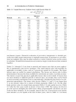
directly from Propositions 24, 25 and 27. The values obtained are listed in Table 1,
where ε = (−1/ p) and thus ε = ±1 according as p ≡ ±1 mod 4.
It will be observed that each of the three symmetric matrices in Table 1 is a
Hadamard matrix! In particular, in each row after the first row of +’s there are equally
many + and − signs. This property turns out to be of basic importance and prompts
the following definition:
A field F is a Hilbert field if some a ∈ F × is not a square and if, for every such a,
the subgroup G a has index 2 in F × .
Thus the real field R = Q∞ and the p-adic fields Q p are all Hilbert fields. We now
show that in Hilbert fields further properties of the Hilbert symbol may be derived.
Proposition 28 A field F is a Hilbert field if and only if some a ∈ F × is not a square

and the Hilbert symbol has the following additional properties:
(i) if (a, b) F = 1 for every b ∈ F × , then a is a square in F × ;
(ii) (a, bc) F = (a, b) F (a, c) F for all a, b, c ∈ F × .
Proof Let F be a Hilbert field. Then (i) holds, since G a = F × if a is not a square.
If (a, b) F = 1 or (a, c) F = 1, then (ii) follows from Proposition 23(v). Suppose
now that (a, b) F = −1 and (a, c) F = −1. Then a is not a square and f a does not
represent b or c. Since F is a Hilbert field and b, c ∈
/ G a , it follows that bc ∈ G a . Thus
(a, bc) F = 1. The converse is equally simple.
✷


2 The Hilbert Symbol

307

Table 1. Values of the Hilbert symbol (a, b) F for F = Qv
Q∞ = R
a\b
1
−1

Q p : p odd

1 −1
+ +
+ −

a\b
1

p
rp
r

1
+
+
+
+

p
+
ε
−ε
−

rp
+
−ε
ε
−

r
+
−
−
+

where r is a primitive root mod p and
ε = (−1)( p−1)/2

Q2
a\b
1
3
6
2
14
10
5
7

1
+
+
+
+
+
+
+
+

3
+
−
+
−
+
−
+
−

6
+
+
−
−
+
+
−
−

2
+
−
−
+
+
−
−
+

14
+
+
+
+
−
−
−
−

10
+
−
+
−
−
+
−
+

5
+
+
−
−
−
−
+
+

7
+
−
−
+
−
+
+
−

The definition of a Hilbert field can be reformulated in terms of quadratic forms. If
f is an anisotropic binary quadratic form with determinant d, then −d is not a square
and f is equivalent to a diagonal form a(ξ 2 + dη2 ). It follows that F is a Hilbert field
if and only if there exists an anisotropic binary quadratic form and for each such form
there is, apart from equivalent forms, exactly one other whose determinant is in the
same square class. We are going to show that Hilbert fields can also be characterized
by means of quadratic forms in 4 variables.
Lemma 29 Let F be an arbitrary field and a, b elements of F × with (a, b) F = −1.
Then the quadratic form
f a,b = ξ12 − aξ22 − b(ξ32 − aξ42 )
is anisotropic. Morover, the set G a,b of all elements of F × which are represented by
f a,b is a subgroup of F × .
Proof Since (a, b) F = −1, a is not a square and hence the binary form f a is
anisotropic. If fa,b were isotropic, some c ∈ F × would be represented by both f a
and b f a . But then (a, c) F = 1 and (a, bc) F = 1. Since (a, b) F = −1, this contradicts
Proposition 23.
Clearly if c ∈ G a,b , then also c−1 ∈ G a,b , and it is easily verified that if
ζ1 = ξ1 η1 + aξ2 η2 + bξ3 η3 − abξ4η4 , ζ2 = ξ1 η2 + ξ2 η1 − bξ3 η4 + bξ4 η3 ,
ζ3 = ξ1 η3 + ξ3 η1 + aξ2 η4 − aξ4 η2 ,

ζ4 = ξ1 η4 + ξ4 η1 + ξ2 η3 − ξ3 η2 ,


308

VII The Arithmetic of Quadratic Forms

then
ζ12 − aζ22 − bζ32 + abζ42 = (ξ12 − aξ22 − bξ32 + abξ42)(η12 − aη22 − bη32 + abη42).

It follows that G a,b is a subgroup of F × .

✷

Proposition 30 A field F is a Hilbert field if and only if one of the following mutually
exclusive conditions is satisfied:
(A) F is an ordered field and every positive element of F is a square;
(B) there exists, up to equivalence, one and only one anisotropic quaternary quadratic
form over F.
Proof Suppose first that the field F is of type (A). Then −1 is not a square, since
−1 + 1 = 0 and any nonzero square is positive. By Proposition 10, any anisotropic
binary quadratic form is equivalent over F to exactly one of the forms ξ 2 +η2 , −ξ 2 −η2
and therefore F is a Hilbert field. Since the quadratic forms ξ12 + ξ22 + ξ32 + ξ42 and
−ξ12 − ξ22 − ξ32 − ξ42 are anisotropic and inequivalent, the field F is not of type (B).
Suppose next that the field F is of type (B). The anisotropic quaternary quadratic
form must be universal, since it is equivalent to any nonzero scalar multiple. Hence,
for any a ∈ F × there exists an anisotropic diagonal form
−aξ12 − b ξ22 − c ξ32 − d ξ42 ,
where b , c , d ∈ F × . In particular, for a = −1, this shows that not every element
of F × is a square. The ternary quadratic form h = −b ξ22 − c ξ32 − d ξ42 is certainly
anisotropic. If h does not represent 1, the quaternary quadratic form −ξ12 + h is also
anisotropic and hence, by Witt’s cancellation theorem, a must be a square. Consequently, if a ∈ F × is not a square, then there exists an anisotropic form
−aξ12 + ξ22 − bξ32 − cξ42 .
Thus for any a ∈ F × which is not a square, there exists b ∈ F × such that
(a, b) F = −1. If (a, b) F = (a, b ) F = −1 then, by Lemma 29, the forms
ξ12 − aξ22 − b(ξ32 − aξ42 ), ξ12 − aξ22 − b (ξ32 − aξ42 )
are anisotropic and thus equivalent. It follows from Witt’s cancellation theorem that
the binary forms b(ξ32 − aξ42 ) and b (ξ32 − aξ42 ) are equivalent. Consequently ξ32 − aξ42
represents bb and (a, bb ) F = 1. Thus G a has index 2 in F × for any a ∈ F × which
is not a square, and F is a Hilbert field.

Suppose now that F is a Hilbert field. Then there exists a ∈ F × which is not a
square and, for any such a, there exists b ∈ F × such that (a, b) F = −1. Consequently,
by Lemma 29, the quaternary quadratic form f a,b is anisotropic and represents 1. Conversely, any anisotropic quaternary quadratic form which represents 1 is equivalent to
some form
g = ξ12 − aξ22 − b(ξ32 − cξ42 )


2 The Hilbert Symbol

309

with a, b, c ∈ F × . Evidently a and c are not squares, and if d is represented by
ξ32 −cξ42 , then bd is not represented by ξ12 −aξ22 . Thus (c, d) F = 1 implies (a, bd) F =
−1. In particular, (a, b) F = −1 and hence (c, d) F = 1 implies (a, d) F = 1.
By interchanging the roles of ξ12 − aξ22 and ξ32 − cξ42 , we see that (a, d) F = 1 also
implies (c, d) F = 1. Hence (ac, d) F = 1 for all d ∈ F × . Thus ac is a square and g is
equivalent to
f a,b = ξ12 − aξ22 − b(ξ32 − aξ42 ).
We now show that f a,b and f a ,b are equivalent if (a, b) F = (a , b ) F = −1.
Suppose first that (a, b ) F = −1. Then (a, bb ) F = 1 and there exist x 3 , x 4 ∈ F such
that b = b(x 32 − ax 42 ). Since
(x 32 − ax 42 )(ξ32 − aξ42 ) = η32 − aη42 ,
where η3 = x 3 ξ3 + ax 4ξ4 , η4 = x 4 ξ3 + x 3 ξ4 , it follows that f a,b is equivalent to f a,b .
For the same reason f a,b is equivalent to f a ,b and thus f a,b is equivalent to f a ,b . By
symmetry, the same conclusion holds if (a , b) F = −1. Thus we now suppose
(a, b ) F = (a , b) F = 1.
But then (a, bb ) F = (a , bb ) F = −1 and so, by what we have already proved,
f a,b ∼ fa,bb ∼ fa ,bb ∼ f a ,b .
Together, the last two paragraphs show that if F is a Hilbert field, then all
anisotropic quaternary quadratic forms which represent 1 are equivalent. Hence the

Hilbert field F is of type (B) if every anisotropic quaternary quadratic form represents 1.
Suppose now that some anisotropic quaternary quadratic form does not represent 1.
Then some scalar multiple of this form represents 1, but is not universal. Thus f a,b is
not universal for some a, b ∈ F × with (a, b) F = −1. By Lemma 29, the set G a,b of
all c ∈ F × which are represented by f a,b is a subgroup of F × . In fact G a,b = G a ,
since G a ⊆ G a,b , G a,b = F × and G a has index 2 in F × . Since fa,b ∼ fb,a , we have
also G a,b = G b . Thus (a, c) F = (b, c) F for all c ∈ F × , and hence (ab, c) F = 1 for
all c ∈ F × . Thus ab is a square and (a, a) F = (a, b) F = −1. Since (a, −a) F = 1, it
follows that (a, −1) F = −1. Hence f a,b ∼ f a,a ∼ fa,−1 . Replacing a, b by −1, a we
now obtain (−1, −1) F = −1 and f a,−1 ∼ f−1,−1 .
Thus the form
f = ξ12 + ξ22 + ξ32 + ξ42
is not universal and the subgroup P of all elements of F × represented by f coincides
with the set of all elements of F × represented by ξ 2 + η2 . Hence P + P ⊆ P and P
is the set of all c ∈ F × such that (−1, c) F = 1. Consequently −1 ∈
/ P and F is the
disjoint union of the sets {O}, P and −P. Thus F is an ordered field with P as the set
of positive elements.
For any c ∈ F × , c2 ∈ P. It follows that if a, b ∈ P then (−a, −b) F = −1,
since aξ 2 + bη2 does not represent −1. Hence it follows that, if a, b ∈ P,


310

VII The Arithmetic of Quadratic Forms

then (−a, −b) F = −1 = (−1, −b) F and (−a, b) F = 1 = (−1, b) F . Thus, for
all c ∈ F × , (−a, c) F = (−1, c) F and hence (a, c) F = 1. Therefore a is a square and
the Hilbert field F is of type (A).
✷

Proposition 31 If F is a Hilbert field of type (B), then any quadratic form f in more
than 4 variables is isotropic.
For any prime p, the field Q p of p-adic numbers is a Hilbert field of type (B).
Proof The quadratic form f is equivalent to a diagonal form a1 ξ12 +· · ·+an ξn2 , where
n > 4. If g = a1 ξ12 + · · · + a4 ξ42 is isotropic, then so also is f . If g is anisotropic then,
since F is of type (B), it is universal and represents −a5 . This proves the first part of
the proposition.
We already know that Q p is a Hilbert field and we have already shown, after the
proof of Corollary VI.17, that Q p is not an ordered field. Hence Q p is a Hilbert field of
type (B).
✷
Proposition 10 shows that two non-singular quadratic forms in n variables, with
coefficients from a Hilbert field of type (A), are equivalent over F if and only if they
have the same positive index. We consider next the equivalence of quadratic forms
with coefficients from a Hilbert field of type (B). We will show that they are classified
by their determinant and their Hasse invariant.
If a non-singular quadratic form f , with coefficients from a Hilbert field F, is
equivalent to a diagonal form a1 ξ12 + · · · + an ξn2 , then its Hasse invariant is defined to
be the product of Hilbert symbols
sF ( f ) =

(a j , ak ) F .
1≤ j
We write s p ( f ) for s F ( f ) when F = Q p . (It should be noted that some authors define
the Hasse invariant with j ≤k in place of j indeed an invariant of f , and for this we make use of Witt’s chain equivalence theorem:
Lemma 32 Let V be a non-singular quadratic space over an arbitrary field F. If
B = {u 1 , . . . , u n } and B = {u 1 , . . . , u n } are both orthogonal bases of V , then there
exists a chain of orthogonal bases B0 , B1 , . . . , Bm , with B0 = B and Bm = B ,

such that B j −1 and B j differ by at most 2 vectors for each j ∈ {1, . . . , m}.
Proof Since there is nothing to prove if dim V = n ≤ 2, we assume that n ≥ 3 and
the result holds for all smaller values of n. Let p = p(B) be the number of nonzero
coefficients in the representation of u 1 as a linear combination of u 1 , . . . , u n . Without
loss of generality we may suppose
p

u1 =

aju j,
j =1

where a j = 0 (1 ≤ j ≤ p). If p = 1, we may replace u 1 by u 1 and the result now
follows by applying the induction hypothesis to the subspace of all vectors orthogonal
to u 1 . Thus we now assume p ≥ 2. We have


2 The Hilbert Symbol

311

a12 (u 1 , u 1 ) + · · · + a 2p (u p , u p ) = (u 1 , u 1 ) = 0,
and each summand on the left is nonzero. If the sum of the first two terms is zero, then
p > 2 and either the sum of the first and third terms is nonzero or the sum of the second
and third terms is nonzero. Hence we may suppose without loss of generality that
a12 (u 1 , u 1 ) + a22 (u 2 , u 2 ) = 0.
If we put
v 1 = a1 u 1 + a2 u 2 ,

v 2 = u 1 + bu 2 ,

vj = uj

for 3 ≤ j ≤ n,

where b = −a1 (u 1 , u 1 )/a2 (u 2 , u 2 ), then B1 = {v 1 , . . . , v n } is an orthogonal basis
and u 1 = v 1 + a3 v 3 + · · · + a p v p . Thus p(B1 ) < p(B). By replacing B by B1 and
repeating the procedure, we must arrive after s < n steps at an orthogonal basis Bs for
which p(Bs ) = 1. The induction hypothesis can now be applied to Bs in the same way
as for B.
✷
Proposition 33 Let F be a Hilbert field. If the non-singular diagonal forms
a1 ξ12 + · · · + an ξn2 and b1 ξ12 + · · · + bn ξn2 are equivalent over F, then
(a j , ak ) F =
1≤ j
(b j , bk ) F .
1≤ j
Proof Suppose first that n = 2. Since a1 ξ12 + a2 ξ22 represents b1 , ξ12 + a1−1 a2 ξ22 represents a1−1 b1 and hence (−a1−1 a2 , a1−1 b1 ) F = 1. Thus (a1 b1 , −a1 a2 b12 ) F = 1 and
hence (a1 b1 , a2 b1 ) F = 1. But (Proposition 28 (ii)) the Hilbert symbol is multiplicative,
since F is a Hilbert field. It follows that (a1 , a2 ) F (b1 , a1 a2 b1 ) F = 1. Since the determinants a1 a2 and b1 b2 are in the same square class, this implies (a1 , a2 ) F = (b1 , b2 ) F ,
as we wished to prove.
Suppose now that n > 2. Since the Hilbert symbol is symmetric, the product
1≤ j Lemma 32 that we may restrict attention to the case where a1 ξ12 + a2 ξ22 is equivalent to b1 ξ12 + b2 ξ22 and a j = b j for all j > 2. Then (a1 , a2 ) F = (b1 , b2 ) F , by what
we have already proved, and it is enough to show that
(a1 , c) F (a2 , c) F = (b1 , c) F (b2 , c) F

for any c ∈ F × .

But this follows from the multiplicativity of the Hilbert symbol and the fact that a1 a2
and b1 b2 are in the same square class.
✷
Proposition 33 shows that the Hasse invariant is well-defined.
Proposition 34 Two non-singular quadratic forms in n variables, with coefficients
from a Hilbert field F of type (B), are equivalent over F if and only if they have the
same Hasse invariant and their determinants are in the same square class.
Proof Only the sufficiency of the conditions needs to be proved. Since this is trivial
for n = 1, we suppose first that n = 2. It is enough to show that if
f = a(ξ12 + dξ22 ),

g = b(η12 + dη22 ),


312

VII The Arithmetic of Quadratic Forms

where (a, ad) F = (b, bd) F , then f is equivalent to g. The hypothesis implies
(−d, a) F = (−d, b) F and hence (−d, ab) F = 1. Thus ξ12 + dξ22 represents ab and
f represents b. Since det f and det g are in the same square class, it follows that f is
equivalent to g.
Suppose next that n ≥ 3 and the result holds for all smaller values of n. Let
f (ξ1 , . . . , ξn ) and g(η1 , . . . , ηn ) be non-singular quadratic forms with det f = det g =
d and s F ( f ) = s F (g). By Proposition 31, the quadratic form
h(ξ1 , . . . , ξn , η1 , . . . , ηn ) = f (ξ1 , . . . , ξn ) − g(η1 , . . . , ηn )
is isotropic and hence, by Proposition 7, there exists some a1 ∈ F × which is represented by both f and g. Thus
f ∼ a1 ξ12 + f ∗ ,

g ∼ a1 η12 + g ∗ ,

where
f ∗ = a2 ξ22 + · · · + an ξn2 ,

g ∗ = b2 η22 + · · · + bn ηn2 .

Evidently det f ∗ and det g ∗ are in the same square class and s F ( f ) = cs F ( f ∗ ),
s F (g) = c s F (g ∗ ), where
c = (a1 , a2 · · · an ) F = (a1 , a1 ) F (a1 , d) F = (a1 , b2 · · · bn ) F = c .
Hence s F ( f ∗ ) = s F (g ∗ ). It follows from the induction hypothesis that f ∗ ∼ g ∗ , and
so f ∼ g.
✷

3 The Hasse–Minkowski Theorem
Let a, b, c be nonzero squarefree integers which are relatively prime in pairs. It was
proved by Legendre (1785) that the equation
ax 2 + by 2 + cz 2 = 0
has a nontrivial solution in integers x, y, z if and only if a, b, c are not all of the same
sign and the congruences
u 2 ≡ −bc mod a,

v 2 ≡ −ca mod b,

w2 ≡ −ab mod c

are all soluble.
It was first completely proved by Gauss (1801) that every positive integer which is
not of the form 4n (8k + 7) can be represented as a sum of three squares. Legendre had
given a proof, based on the assumption that if a and m are relatively prime positive

integers, then the arithmetic progression
a, a + m, a + 2m, . . .
contains infinitely many primes. Although his proof of this assumption was faulty,
his intuition that it had a role to play in the arithmetic theory of quadratic forms


3 The Hasse–Minkowski Theorem

313

was inspired. The assumption was first proved by Dirichlet (1837) and will be
referred to here as ‘Dirichlet’s theorem on primes in an arithmetic progression’. In
the present chapter Dirichlet’s theorem will simply be assumed, but it will be proved
(in a quantitative form) in Chapter X.
It was shown by Meyer (1884), although the published proof was incomplete, that
a quadratic form in five or more variables with integer coefficients is isotropic if it is
neither positive definite nor negative definite.
The preceding results are all special cases of the Hasse–Minkowski theorem, which
is the subject of this section. Let Q denote the field of rational numbers. By Ostrowski’s
theorem (Proposition VI.4), the completions Qv of Q with respect to an arbitrary absolute value | |v are the field Q∞ = R of real numbers and the fields Q p of p-adic
numbers, where p is an arbitrary prime. The Hasse–Minkowski theorem has the
following statement:
A non-singular quadratic form f (ξ1 , . . . , ξn ) with coefficients from Q is isotropic
in Q if and only if it is isotropic in every completion of Q.
This concise statement contains, and to some extent conceals, a remarkable amount
of information. (Its equivalence to Legendre’s theorem when n = 3 may be established
by elementary arguments.) The theorem was first stated and proved by Hasse (1923).
Minkowski (1890) had derived necessary and sufficient conditions for the equivalence
over Q of two non-singular quadratic forms with rational coefficients by using known
results on quadratic forms with integer coefficients. The role of p-adic numbers was

taken by congruences modulo prime powers. Hasse drew attention to the simplifications obtained by studying from the outset quadratic forms over the field Q, rather
than the ring Z, and soon afterwards (1924) he showed that the theorem continues to
hold if the rational field Q is replaced by an arbitrary algebraic number field (with its
corresponding completions).
The condition in the statement of the theorem is obviously necessary and it is only
its sufficiency which requires proof. Before embarking on this we establish one more
property of the Hilbert symbol for the field Q of rational numbers.
Proposition 35 For any a, b ∈ Q× , the number of completions Qv for which one has
(a, b)v = −1 (where v denotes either ∞ or an arbitrary prime p) is finite and even.
Proof By Proposition 23, it is sufficient to establish the result when a and b are
square-free integers such that ab is also square-free. Then (a, b)r = 1 for any
odd prime r which does not divide ab, by Proposition 25. We wish to show that
v (a, b)v = 1. Since the Hilbert symbol is multiplicative, it is sufficient to establish this in the following special cases: for a = −1 and b = −1, 2, p; for a = 2 and
b = p; for a = p and b = q, where p and q are distinct odd primes. But it follows
from Propositions 24, 25 and 27 that
(−1, −1)v = (−1, −1)∞ (−1, −1)2 = (−1)(−1) = 1;
v

(−1, 2)v = (−1, 2)∞ (−1, 2)2 = 1 · 1 = 1;
v


314

VII The Arithmetic of Quadratic Forms

(−1, p)v = (−1, p) p (−1, p)2 = (−1/ p)(−1)( p−1)/2;
v

(2, p)v = (2, p) p (2, p)2 = (2/ p)(−1)( p

2 −1)/8

;

v

( p, q)v = ( p, q) p ( p, q)q ( p, q)2 = (q/ p)( p/q)(−1)( p−1)(q−1)/4.
v

Hence the proposition holds if and only if
(−1/ p) = (−1)( p−1)/2, (2/ p) = (−1)( p

2 −1)/8

, (q/ p)( p/q) = (−1)( p−1)(q−1)/4.

Thus it is actually equivalent to the law of quadratic reciprocity and its two
‘supplements’.
✷
We are now ready to prove the Hasse–Minkowski theorem:
Theorem 36 A non-singular quadratic form f (ξ1 , . . . , ξn ) with rational coefficients
is isotropic in Q if and only if it is isotropic in every completion Qv .
Proof We may assume that the quadratic form is diagonal:
f = a1 ξ12 + · · · + an ξn2 ,
where ak ∈ Q× (k = 1, . . . , n). Moreover, by replacing ξk by rk ξk , we may assume
that each coefficient ak is a square-free integer.
The proof will be broken into three parts, according as n = 2, n = 3 or n ≥ 4. The
proofs for n = 2 and n = 3 are quite independent. The more difficult proof for n ≥ 4
uses induction on n and Dirichlet’s theorem on primes in an arithmetic progression.

(i) n = 2: We show first that if a ∈ Q× is a square in Q×
v for all v, then a is already
α p be the
a square in Q× . Since a is a square in Q×
∞ , we have a > 0. Let a =
p p
factorization of a into powers of distinct primes, where α p ∈ Z and α p = 0 for at most
finitely many primes p. Since |a| p = p −α p and a is a square in Q p , α p must be even.
But if α p = 2β p then a = b 2 , where b = p pβ p .
Suppose now that f = a1 ξ12 + a2 ξ22 is isotropic in Qv for all v. Then a := −a1 a2
is a square in Qv for all v and hence, by what we have just proved, a is a square in Q.
But if a = b2 , then a1 a22 + a2 b2 = 0 and thus f is isotropic in Q.
(ii) n = 3: By replacing f by −a3 f and ξ3 by a3 ξ3 , we see that it is sufficient to prove
the theorem for
f = aξ 2 + bη2 − ζ 2 ,
where a and b are nonzero sq� · · ,
where a, b, c ∈ F p and the unwritten terms are of degree > 2. Otherwise, the singular
point is a node.
For any prime p, let N p denote the number of F p -points of W p , including the point
at infinity O, and put
cp = p + 1 − Np.
It was conjectured by Artin (1924), and proved by Hasse (1934), that
|c p | ≤ 2 p 1/2

if p ∆.

Since 2 p1/2 is not an integer, this inequality says that the quadratic polynomial
1 − c p T + pT 2
has conjugate complex roots γ p , γ¯ p of absolute value p−1/2 or, if we put T = p −s ,
that the zeros of

1 − c p p−s + p 1−2s
lie on the line Rs = 1/2. Thus it is an analogue of the Riemann hypothesis on the zeros
of ζ (s), but differs from it by having been proved. (As mentioned in §5 of Chapter IX,
Hasse’s result was considerably generalized by Weil (1948) and Deligne (1974).)
The L-function of the original elliptic curve W is defined by
(1 − c p p−s )−1

L(s) = L(s, W ) :=
p|∆

(1 − c p p−s + p 1−2s )−1 .
p∆

The first product on the right side has only finitely many factors. The infinite second
product is convergent for Rs > 3/2, since
1 − c p p−s + p 1−2s = ( p1/2−s − p 1/2 γ p )( p 1/2−s − p 1/2 γ¯ p )


572

XIII Connections with Number Theory

and |γ p | = |γ¯ p | = p−1/2 . Multiplying out the products, we obtain for Rs > 3/2
an absolutely convergent Dirichlet series
cn n −s

L(s) =
n≥1

with integer coefficients cn . (If n = p is prime, then cn is the previously defined c p .)

The conductor N = N(W ) of the elliptic curve W is defined by the singular
reductions W p of W :
p fp,

N=
p|∆

where f p = 1 if W p has a node, whereas f p = 2 if p > 3 and W p has a cusp. We
will not define f p if p ∈ {2, 3} and W p has a cusp, but we mention that f p is then an
integer ≥ 2 which can be calculated by an algorithm due to Tate (1975). (It may be
shown that f2 ≤ 8 and f3 ≤ 5.)
The elliptic curve W is said to be semi-stable if W p has a node for every p|∆. Thus,
for a semi-stable elliptic curve, the conductor N is precisely the product of the distinct
primes dividing the discriminant ∆. (The semi-stable case is the only one in which the
conductor is square-free.)
Three important conjectures about elliptic curves, involving their L-functions and
conductors, will now be described.
It was conjectured by Hasse (1954) that the function
ζ (s, W ) := ζ(s)ζ (s − 1)/L(s, W )
may be analytically continued to a function which is meromorphic in the whole
complex plane and that ζ (2 − s, W ) is connected with ζ(s, W ) by a functional
equation similar to that satisfied by the Riemann zeta-function ζ(s). In terms of
L-functions, Hasse’s conjecture was given the following precise form by Weil (1967):
HW-Conjecture: If the elliptic curve W has L-function L(s) and conductor N, then
L(s) may be analytically continued, so that the function
Λ(s) = (2π)−s Γ (s)L(s),
where Γ (s) denotes Euler’s gamma-function, is holomorphic throughout the whole
complex plane and satisfies the functional equation
Λ(s) = ±N 1−s Λ(2 − s).
(In fact it is the functional equation which determines the precise definition of the

conductor.)
The second conjecture, due to Birch and Swinnerton-Dyer (1965), connects the
L-function with the group of rational points:
BSD-Conjecture: The L-function L(s) of the elliptic curve W has a zero at s = 1 of
order exactly equal to the rank r ≥ 0 of the group E = E(W , Q) of all rational points
of W .