Ebook Quantum theory of magnetism - Magnetic properties of materials (3/E): Part 2
Bạn đang xem bản rút gọn của tài liệu. Xem và tải ngay bản đầy đủ của tài liệu tại đây (7.86 MB, 190 trang )
5
The Static Susceptibility
of Interacting Systems: Metals
The long-range magnetic order in metals is very similar to that observed in insulators as illustrated by the magnetization curve of nickel shown in Fig. 5.1.
However, the electrons participating in this magnetic state are itinerant as
determined by the existence of a Fermi surface; that is, they also have translational degrees of freedom. How such a system of interacting electrons responds
to a magnetic field is a many-body problem with all its attendant difficulties.
The many-body corrections to the Landau susceptibility and the Pauli
susceptibility must be treated separately. Kanazawa and Matsudaira [104]
found that the many-body corrections to the Landau susceptibility are small
(less than one per cent) for high electron densities.
We shall approach the effect of electron-electron interactions on the spin
susceptibility in two ways. The first, Fermi liquid theory, is a phenomenological approach. It involves parameters completely analogous to the parameters entering the spin Hamiltonian. These parameters may be determined
experimentally or they may be obtained from the second approach which is to
assume a specific microscopic model from which various physical properties
can be calculated.
5.1 Fermi Liquid Theory
The phenomenological theory of an interacting fermion system was developed
by Landau in 1956 [106]. Although Landau was mainly interested in the properties of liquid He3 , his theory may also be applied to metals. Modifications
of this theory in terms of the introduction of a magnetic field have been made
by Silin [107].
Let us begin by considering the ground state of a system of N electrons.
For a noninteracting system the ground state corresponds to a well-defined
Fermi sphere. Landau assumed that as the interaction between the electrons
is gradually “turned on” the new ground state evolves smoothly out of the
170
5 The Static Susceptibility of Interacting Systems
1.0
M − M 0 ~ T 3/2
0.9
Ni
T c = 632.7 +− 0.4 K
0.8
0.7
M
M0
0.6
0.5
0.4
0.3
0.2
M ~ (T c − T) 0.355
0.1
0
0
1
T/Tc
Fig. 5.1. Magnetization of nickel as a function of temperature. The original data
of Weiss and Forrer [105] taken at constant pressure has been corrected to constant
volume to eliminate the effects of thermal expansion
original Fermi sphere; if |0 is this new ground state, it is related to the original
Fermi sphere |F S by a unitary transformation,
|0 = U |F S .
(5.1)
Let us denote the energy associated with |0 as E0 .
Landau also applied this assumption to the excitations of the interacting
system. For example, suppose we add one electron, with momentum k, to
the non-interacting system. This state has the form a†kσ |F S , where a†kσ is
the creation operator for an electron. If the interactions are gradually turned
on, let us approximate the new state as
|kσ = U a†kσ |F S .
(5.2)
Because the electron possesses spin, this wave function is a spinor.
Let us define the difference between the energy of |kσ and |0 as 0 (k, σ).
Since the wave function is a spinor, this energy will be a 2 × 2 matrix. If the
system is isotropic, and in particular if there is no external magnetic field,
then this energy is independent of the spin,
0
(k, σ)αβ =
0
(k)δαβ .
Because the whole Fermi sphere has readjusted itself as a result of the interactions, the energy 0 (k) will be quite different from the energy of a free
particle. As we do not know this energy, we shall assume that k is close to kF
and expand in powers of k − kF . Thus we obtain
0
2
(k) = µ +
kF
(k − kF ) + . . . ,
m∗
(5.3)
5.1 Fermi Liquid Theory
where
kF
∂ 0 (k)
≡
∗
m
∂k
171
2
.
(5.4)
k=kF
This electron, “dressed” by all the other electrons, is called a quasiparticle.
Notice that the energy required to create a quasiparticle at the Fermi surface
is µ, the chemical potential. Its increase in energy as it moves away from the
Fermi surface is characterized by its effective mass m∗ . We restrict ourselves
to the region close to the Fermi surface because it is only in this region that
quasiparticle lifetimes are long enough to make their description meaningful.
We could just as well have removed an electron from some point within the
Fermi sphere. This would have created a “hole”, which the interactions would
convert into a quasi-hole. The energy associated with a hole is the energy
required to remove an electron at the Fermi surface, −µ, plus the energy
it takes to move the electron at k up to the surface, ( 2 kF /m∗ )(kF − k).
However, if we define the total energy of the system containing a quasi-hole
as E0 − 0 (k), then
2
kF
0
(k) = µ +
|k − kF | .
m∗
Thus the excitation spectrum associated with our Fermi liquid has the form
shown in Fig. 5.2.
Suppose that other quasiparticles are now introduced into the system. This
could occur, for example, as a result of an external field producing electronhole pairs. Since the energy of a quasiparticle depends on the distribution of
all the other quasiparticles, any change in distribution will lead to a change
in the quasiparticle energy. Let us denote the change in the distribution by
δn(k, σ).
The quasiparticle distribution is essentially the density matrix associated with the quasiparticle. In particular, it is a 2 × 2 matrix. For example,
δn(k, σ)11 gives the probability of finding an electron of momentum k with
Excitation
energy
Qu
as
ole
s
a
sip
s
cle
rti
i-h
a
Qu
k
kF
Fig. 5.2. Single-particle excitation spectrum of a Fermi liquid
172
5 The Static Susceptibility of Interacting Systems
spin up. Therefore the quasiparticle energy may be written in phenomenological terms as
(k, σ) =
0
(k, σ) +
1
Tr
V σ
k
f (k, σ; k , σ )δn(k , σ )
.
(5.5)
The quantity f (k, σ; k , σ ) is a product of 2×2 matrices analogous to a dyadic
vector product. Again, if the system is isotropic, the most general form this
quantity can have is
f (k, σ; k , σ ) = ϕ(k, k )11 + ψ(k, k )σ · σ ,
(5.6)
where 1 is the 2 × 2 unit matrix. Furthermore, since this theory is valid only
near the Fermi surface, we may take |k | |k| = kF . Then ϕ and ψ depend
only upon the angle θ between k and k, and we may expand ϕ and ψ in
Legendre polynomials:
ϕ(k, k ) =
2 2
π2 2
ˆ·k
ˆ)= π
A(
k
[A0 + A1 P1 (cos θ) + . . .] ,
m∗ kF
m∗ kF
(5.7)
ψ(k, k ) =
2 2
π2 2
ˆ·k
ˆ)= π
B(k
[B0 + B1 P1 (cos θ) + . . .] .
∗
m kF
m∗ kF
(5.8)
If we know the quasiparticle distribution function, then we can compute, just
as for the electron gas, all the relevant physical quantities. These will involve
the parameters An and Bn . The beauty of this theory is that some of the same
parameters enter different physical quantities. Therefore by measuring certain
quantities we can predict others. The difficulty, of course, is in determining
the distribution function δn(k, σ). For static situations this is relatively easy.
However, for dynamic situations, as we shall see in the following chapters, we
have to solve a Boltzmann-like equation.
Since the k dependence of the quasiparticle energy is a result of interactions, there should be a relation between m∗ and the parameters An and Bn .
To obtain this relation let us consider the situation at T = 0 in which we have
one quasiparticle at k with spin up, as illustrated in Fig. 5.3a. Now, suppose
the momentum of this system is increased by q, giving us the situation in
δ n(k , σ ) = -1
k +q
k
Fermi
Sphere
q
(a)
(b)
δ n(k , σ ) = +1
Fig. 5.3. Effect of a uniform translation in momentum space on a state containing
one extra particle
5.1 Fermi Liquid Theory
173
Fig. 5.3b. This corresponds to placing the whole system on a train moving
with a velocity q/m. To an observer at rest with respect to the train it will
appear that the quasiparticle has acquired an additional energy
2
δ (k, σ)11 =
k · q/m
(5.9)
for small q. However, the quasiparticle itself experiences a change in energy
associated with its own motion in momentum space, which, from (5.3), is just
2
k · q/m∗ . In addition, it sees the redistribution of quasiparticles indicated
in Fig. 5.3b. Since this momentum displacement does not produce any spin
flipping, δn(k, σ)αβ will have the form δn(k)δαβ , where δn(k) is +1 for the
quasiparticles and −1 for the quasi-holes. This gives a contribution of
2
V
ϕ(k, k )δn(k )
k
to the 1,1 component of the energy, where the factor 2 arises from the spin
trace. Equating these two changes in energy, which is what is meant by
Galilean invariance, and converting the sum over k to an integral leads to
our desired relation,
m∗ = m 1 +
A1
3
.
(5.10)
It can be shown that the specific heat of a Fermi liquid has the same form as
that for an ideal Fermi gas, with m replaced by m∗ . Thus by measuring the
specific heat we can determine the Fermi liquid parameter A1 .
Exchange Enhancement of the Pauli Susceptibility. We are now ready to consider our original question of the response of a Fermi liquid to a magnetic
field. In the presence of a magnetic field the noninteracting quasiparticle
energy 0 (k, σ) is no longer independent of the spin, but contains a Zeeman
contribution,
0
(k, σ) = 0 (k)1 + µB Hσz .
(5.11)
We shall assume that any field-induced contributions to the interaction term
are small. Therefore the total quasiparticle energy is
(k, σ) =
0
(k)1 + µB Hσz +
1
Tr
V σ
f (k, σ; k , σ )δn(k σ )
.
(5.12)
k
It is energetically more favorable for the quasiparticles to align themselves
opposite to the field, since their gyromagnetic ratio is negative. However, each
time a quasiparticle flips over it changes the distribution, thereby bringing in
contributions from the last term in (5.12). Thus, if we start with two equal spin
174
5 The Static Susceptibility of Interacting Systems
δk F
δk F
(a)
(b)
Fig. 5.4. Effect of a dc magnetic field on the spin-up and the spin-down Fermi
spheres
distributions, as shown in Fig. 5.4a, an equilibrium situation will eventually be
reached, as illustrated in Fig. 5.4b, in which the energy of a quasiparticle on
the up-spin Fermi surface is equal to that of a quasiparticle on the down-spin
surface; that is,
(kF + δkF , σ)22 = (kF − δkF , σ)11 .
(5.13)
From (5.3), (5.12) this condition becomes
2
kF
1
δkF − µB H + Tr
m∗
V σ
=−
ˆ·k
ˆ )1 − ψ(k
ˆ·k
ˆ )σ δn(k , σ )
ϕ(k
z
k
2
kF
1
δkF + µB H + Tr
m∗
V σ
ˆ·k
ˆ )1 + ψ(k
ˆ·k
ˆ )σ δn(k , σ )
ϕ(k
z
.
k
(5.14)
The change in quasiparticle distribution shown in Fig. 5.4b is characterized by
⎧
00
⎪
⎪
kF < |k| < kF + δkF
⎨ 01
(5.15)
δn(k, σ) =
⎪
−1 0
⎪
⎩
k − δkF < |k| < kF .
00 F
Therefore
ˆ·k
ˆ )1δn (k , σ )
ϕ(k
Tr
σ
= 0,
(5.16)
k
while
ˆ·k
ˆ )σ δn(k , σ)
ψ(k
z
Tr
σ
=−
k
4πV 2
k δkF
(2π)3 F
+1
ˆk
ˆ ) . (5.17)
d(cos θ)ψ(k·
−1
Equation (5.14) then reduces to
2 2 kF δkF
2 2 kF
δk
−
2µ
H
+
B0 = 0 .
F
B
m∗
m∗
(5.18)
5.1 Fermi Liquid Theory
175
Since the magnetization is
Mz = −
µB
Tr
V σ
σz δn(k, σ)
= 2µB
k
πkF2 δkF
.
(2π)3
(5.19)
the uniform susceptibility of a Fermi liquid at T = 0 is
χ(0) =
1 + 13 A1
χPauli .
1 + B0
(5.20)
Thus we find that in addition to the appearance of the effective mass in place
of the bare mass, the susceptibility is also modified by the factor (1 + B0 )−1 .
In the Hartree–Fock approximation
B0 = −
me2
= −0.166rs
π 2 kF
(5.21)
and we speak of the susceptibility as being exchange enhanced. As the electron
density decreases and rs → 6.03 the susceptibility diverges. This is usually
taken to imply that such a material will be ferrogmagnetic. There has been
a great deal of discussion [108] about the magnetic state of an interacting
electron system, and it is generally agreed that such a system will not become
ferromagnetic at any electron density. That is, the Hartree-Fock approximation favors ferromagnetism. The reason is that in this approximation parallel spins are kept apart by the exclusion principle while antiparallel spins
are spatially uncorrelated. Thus the antiparallel spins have a relatively large
Coulomb energy to gain by becoming parallel. In an exact treatment one would
expect the antiparallel spins to be somewhat correlated, thereby reducing the
Coulomb difference. The differences between the exact properties of an interacting electron system and those obtained in the Hartree-Fock approximation
are referred to as correlation effects. Estimates of these correlation corrections
indicate that the nonmagnetic ground state of the electron gas has a lower
energy than the ferromagnetic one.
The predictions of Fermi-liquid theory, namely that the low temperature
heat capcity varies as γT and that the resistivity varies as T 2 are found to
describe most metals. During the last decade, however, non-Fermi-liquid
behavior has been observed in a number of systems. One of the most studied
is the high-temperature superconductor, Laz−x Srx CuO4 . The phase diagram
for this system is shown in Fig. 4.16. The “normal” region above the superconducting region shows anamolous features. Anderson, for example, argues
that the absence of a residual resistivity in the ab plane invalidates a Fermiliquid description. It is known that a Fermi-liquid approach certainly fails
in one dimension, for in one dimension the Fermi “surface” consists of only
two points at k = ±kF . Any interaction with momentum transfer q = 2kF
leads to an instability that produces a gap in the energy spectrum. In 1963
176
5 The Static Susceptibility of Interacting Systems
Luttinger introduced a model of 1D interacting Fermions. His solution does
not give quasiparticles, but rather spin and charge excitations that propagate
independently. Whether the 2D CuO2 planes in La2−x Srx CuO4 can be described by such a “Luttinger liquid” is a subject of debate. Other materials
exhibiting non-Fermi-liquid behavior are the so-called heavy Fermions.
5.2 Heavy Fermion Systems
At low temperatures the electrons in a “normal” metal contribute a term
to the specific heat that is linear in the temperature, i.e., C = γT as we
2
N (EF ).
mentioned above. Simple theoretical considerations give γ = 23 π 2 kB
In particular, for a free electron metal the density of states is given by
1/2
N (EF ) = (2m/ 2 )3/2 EF which gives a value of γ of the order of one
−1
−2
mJ/K mol . There exist, however, metallic systems with low temperature heat capacity coefficients of the order of 1000 mJ/K−2 mol−1 . Examples
include CeCu2 Si2 , UBe13 , and UPt3 . Almost all the examples involve rare
earths, such as Ce, or actinides, such as U. These elements have their f n and
f n±1 electronic configurations close enough in energy to allow valence fluctuations with hybridization. This can lead to Kondo behavior (see Sect. 3.4.3)
and is why some refer to heavy Fermion systems as “Kondo lattices”. In this
description the large electronic mass is associated with a large density of states
at the Fermi level that derives from the many-body resonance we found in our
treatment of the Kondo impurity. When d-electron ions are used to create a
Kondo lattice their large spatial extent results in too strong a hybridization
to show heavy Fermion behavior. LiV2 O4 appears to be an exception.
Once one has a heavy Fermion system it is subject to the same sorts
of Fermi surface instabilities found in more normal metals. In particular,
CeCu2 Si2 shows both a spin density wave and superconductivity as one
changes the 4f-conduction electron coupling by substituting Ge for the Si.
The Kondo lattice is not the only mechanism that may lead to heavy
Fermions. When Nd2 CuO4 is doped with electrons by introducing Ce for Nd,
i.e., Nd2−x Cex CuO4 , the linear specific heat coefficient is γ = 4 J/K−2 mol−1 .
The conduction occurs through hopping among the Cu sites. As a result of
the double exchange we described in Sect. 2.2.10, these hopping electrons see
an effective antiferromagnetic field. The conduction electron Hamiltonian is
therefore taken to be
(a†iσ ajσ + h.c.) + h
−t
i,j,σ
σeiQ·Ri a†iσ aiσ ,
iσ
where Q is a reciprocal lattice vector (π/a, π/a) and h is the effective field that
accounts for the antiferromagnetic correlations. The 4f electrons are described
by the term
†
fiσ
fiσ .
f
iσ
5.3 Itinerant Magnetism
177
Fig. 5.5. Schematic plot of the quasiparticle bands of Ndz−x Cex CuO4 for x = 0.
The Fermi energy is indicated by a dotted line. Solid lines: f -like excitations, and
dashed lines: d-like excitations [109]
Finally, we add a hybridization
(a†iσ fiσ + h.c.) .
V
iσ
This is a very simplified model since it only considers one 4f orbital instead of
seven. Nevertheless, when this Hamiltonian is diagonalized [109] one obtains
the four bands shown in Fig. 5.5. The Fermi level in the doped case sits in the
narrow f -band giving rise to a large electronic mass.
5.3 Itinerant Magnetism
The appearance of ferromagnetism in real metals is related to the presence of
the ionic cores which tend to localize the intinerant electrons and introduce
structure in the electronic density of states. We shall now consider two models
that incorporate these features.
5.3.1 The Stoner Model
In the 1930s both Slater [110] and Stoner [111] combined Fermi statistics
with the molecular field concept to explain itinerant ferromagnetism. This
one-electron approach is now generally referred to as the Stoner model. It
bears similarities to Landau’s Fermi liquid theory in that the effect of the
electron-electron interactions is to produce a spin-dependent potential that
simply shifts the original Bloch states.
Stoner’s result is contained within the generalized susceptibility χ(q) of an
interacting electron system. As a model Hamiltonian we take a form similar
to (1.139) where k now refers to the Bloch band energy. Since the Coulomb
interaction in a metal is screened, let us take a delta-function interaction of
178
5 The Static Susceptibility of Interacting Systems
the form Iδ(r i −r j ). In this case one need not add a compensating background
charge density and (1.139) becomes
†
k akσ akσ
H0 =
+
kσ
I
V
a†k−q,σ a†k +q,−σ ak,σ ak σ . (5.22)
k
k
q
k
σ
ˆ cos(q · r), the Zeeman Hamiltonian
If we now add a spatially varying field H z
becomes
H
(5.23)
HZ = − [Mz (q) + Mz (−q)] ,
2
where
1
a†k−q,↑ ak↑ − a†k−q,↓ ak↓ .
(5.24)
Mz (q) = gµB
2
k
Susceptibility. The susceptibility is obtained by calculating the average value
of Mz (q) to lowest order in H. In particular, we must calculate the average of
mk,q ≡ a†k−q,↑ ak,↑ − a†k−q,↓ ak,↓ .
Following Wolff [112] we shall do this by writing the equation of motion for
mk,q and using the fact that in equilibrium ∂ mk,q ∂t = 0. Thus,
[mk,q , H0 + HZ ] = 0 .
(5.25)
This commutator involves a variety of twofold and fourfold products of electron operators. These are simplified by making a random-phase approximation in which we retain only those pairs which are diagonal or have the forms
appearing in mk,q itself. Furthermore, the diagonal pairs are replaced by their
average in the noninteracting ground state. This is equivalent to a HartreeFock approximation. The result is
( k−
k+q )
mk,q −
Dividing by (
k+q
−
2I
(nk+q −nk )
V
k)
mk ,q −gµB H(nk+q −nk ) = 0 . (5.26)
k
and summing over k gives
gµB H
mk,q =
k
1−
2I
V
k
k
nk − nk+q
k+q − k
.
nk − nk+q
k+q − k
(5.27)
Since the equilibrium occupation number nk is just the Fermi function fk ,
we recognize the sum appearing in this expression as the same as that which
appears in the noninteracting susceptibility (3.93), which we shall denote as
χ0 (q). Thus,
5.3 Itinerant Magnetism
χ(q) =
χ0 (q)
.
1 − g22Iµ2 χ0 (q)
179
(5.28)
B
We could also have calculated mk,q directly by the formulation indicated in
(1.81). However, the appearance of the interaction term in the exponentials
which enter mk,q (t) requires many-body perturbation techniques which are
beyond the scope of this monograph. We shall use the diagrams introduced
in Chap. 1 to make the results of such a treatment plausible. The interaction
term in (5.22) has the diagramatic form
In calculating average values such as the energy or the magnetization the
electron and hole lines must be closed.
There are two ways one can close the electron and hole lines:
In (a) the vertices indicated by the small squares involve a momentum change
q but no spin flip. This longitudinal spin fluctuation represents the first-order
correction to χzz . The susceptibility (5.28) corresponds to the summation of
all such diagrams:
In diagram (b) the vertices also involve a spin flip. This diagram is the firstorder correction to the transverse susceptibility χ−+ (q) whose noninteracting
form is given by (3.97). Summing all such transverse spin fluctuations gives
the transverse susceptibility.
180
5 The Static Susceptibility of Interacting Systems
In the paramagnetic state rotational invariance requires χ−+ (q) = 2χzz (q).
Returning to (5.28), since limq→0 χ0 (q) = 13 g 2 µ2B D( F ), we see that
χ(0) =
χ0 (0)
.
1 − ID( F )
(5.29)
This has the same form as our Fermi liquid result (5.20). Thus we have an
expression, at least in the random-phase approximation, for the Fermi liquid
parameter B0 in terms of the intraatomic exchange integral I and the density
of states.
Notice that the criterion for the appearance of ferromagnetism is that
ID( F ) ≥ 1. This is referred to as the Stoner criterion.
One might wonder how ferromagnetism can occur with only an intraatomic
Coulomb interaction. To see the physical origin of this, suppose we have a
spin up at some site α. If the spin on a neighboring site α is also up, it
is forbidden by the exclusion principle from hopping onto site α. Therefore
the two electrons do not interact, and we might define the energy of such a
configuration as 0. However, if the spin of site α is down, it has a nonzero
probability of hopping onto site α. Thus the energy of this configuration is
higher than that of the “ferromagnetic” one. However, hopping around can
lower the kinetic energy of the electrons. This is reflected in the appearance of
the density of states in the Stoner criterion. The occurrence of ferromagnetism
depends, therefore, on the relative values of the Coulomb interaction and the
kinetic energy.
Equation (5.29) has interesting consequences for metals which are paramagnetic but have a large enhancement factor. For example, an impurity spin
placed in such a host produces a large polarization of the conduction electrons in its vicinity. Such giant moments have been observed in palladium
and certain of its alloys. This seems reasonable, since palladium falls just
below nickel in the periodic table and has similar electronic properties. Thus
we might suspect that although palladium is not ferromagnetic like nickel, it
at least possesses a large exchange enhancement.
Spin-Density Waves. Just as in the case of localized moments, a divergence
of χ(q) for q = 0 would imply a transition to a state of nonuniform magnetization. In fact, Overhauser [113] has shown that the χ(q) associated with
an unscreened Coulomb interaction in the Hartree-Fock approximation does
diverge as q → 2kF , as shown in Fig. 5.6. This would lead to a ground state
characterized by a period spin density, called a spin-density wave. The effects
of screening and electron correlations, however, tend to suppress this divergence. Consequently, a spin-density wave can form only under rather special conditions. We get some feeling for these conditions by considering the
behavior of the non-interacting susceptibility χ0 (q) in one and two dimensions
5.3 Itinerant Magnetism
181
Fig. 5.6. Effect of electron-electron interactions on the susceptibility (3 dimensions)
Fig. 5.7. Effect of dimensionality on the free electron susceptibility
as shown in Fig. 5.7. We see that lower dimensional systems are more likely
to become unstable with respect to spin-density wave formation.
The reason for this has to do with the fact that in a state characterized
by a wave vector q electrons with wave vectors which differ by q become
correlated. This effectively removes them from the Fermi sea. This is often
described as a “nesting” of the corresponding states. In one and two dimensions Fermi surfaces are geometrically simpler, which means that nesting will
have more dramatic effects. These same considerations, however, also apply
182
5 The Static Susceptibility of Interacting Systems
to charge-density instabilities. And, in fact, most of the materials which do
show such Fermi-surfaced-related instabilities show charge-density waves.
To date, chromium and its alloys are the best examples of materials possessing a spin-density-wave ground state. The reason for this has to do with
the band structure of chromium.
If the susceptibility does not actually diverge at some nonzero wave vector,
but nevertheless becomes very large, the system may be said to exhibit antiferromagnetic exchange enhancement. Experiments on dilute alloys of Sc:Gd
indicate that scandium metal may be an example of such a type [114].
Exchange Splitting. If the system is ferromagnetic, then mk,q=0 = (nk↑ −
nk↓ ) = 0 even in the absence of an applied field. In this case the Hamiltonian may be written in a particularly revealing form by considering only
the diagonal terms in (5.22):
1
1
nk ↓ a†k↑ ak↑ + nk ↑ a†k↓ ak↓ .
2
2
Since
M=
gµB
2V
(5.30)
(nk↑ − nk↓ ) ,
(5.31)
†
kσ akσ akσ
,
(5.32)
IM
NI
−
σ.
4V
2gµB
(5.33)
k
the Hamiltonian becomes
H0 = E0 +
k,σ
where
kσ
=
k
+
Thus the spin-up and spin-down energy bands are split by an amount proportional to the magnetization. This was the basic idea in Stoner’s original
theory of ferromagnetism. More generally, this splitting arises from the difference between the spin-up and spin-down exchange-correlation potentials seen
by the electrons. Since the Stoner model was first proposed there has been a
great deal of progress in specifying these potentials.
In 1951 Slater [115] suggested that we approximate the effect of exchange
by the potential
Vx (r) = −6[(3/8π)ρ(r)]1/3 .
This approximation form has been used extensively both in atomic and solidstate calculations. Physically, this density to the one-third power arises from
the fact that in the Hartree-Fock approximation parallel spins are kept farther
apart than antiparallel spins. Therefore, there is an “exchange hole” around
any particular spin associated with a deficiency of similar spins. The radius
of this hole must be such that ( 34 )πr3 ρ = 1. Since the potential associated
with this deficiency is proportional to 1/r, we obtain an exchange potential
proportional to ρ1/3 .
5.3 Itinerant Magnetism
183
In 1965 Kohn and Sham [116] rederived the exchange potential by a different method and obtained a value two thirds that of Slater’s. This led workers
to multiply Vx (r) by an adjustable constant, α, which can be determined for
each atom by requiring that the so-called Xα energy be equal to the HartreeFock energy for that atom. An interesting application of the Xα method has
been made by Hattox et al. [117]. They calculated the magnetic moment of
bcc vanadium as a function of lattice spacing. The result is shown in Fig. 5.8.
We see that the moment falls suddenly to zero at a spacing 20% larger than
the actual observed spacing. This decrease is due to the broadening of the
3d band as the lattice spacing decreases. This is consistent √
with the fact that
A,
bcc vanadium, where the vanadium-vanadium distance is 3 a0 /2 = 2.49 ˚
is observed to be nonmagnetic. In Au4 V, however, the vanadium-vanadium
distance has increased to 3.78 ˚
A and the vanadium has a moment near one
Bohr magneton.
If one uses this approach to find α for the magnetic transition metals one
finds that the resulting magnetic moments are not in agreement with those
observed.
This is not surprising when we consider that we have replaced a nonlocal
potential (the Hartree-Fock potential) by a local potential (the Slater ρ1/3 ).
Furthermore, the fact that these are different means that the Slater potential
must, by definition, include some correlation. However, we do not know if it
is in the right direction.
The arbitrariness inherent in the Xα method may be avoided by using the
“spin-density functional” formalism. This essentially enables one to utilize
the results of many-body calculations for the homogeneous electron gas in
determining the exchange and correlation potentials in transition metals. This
Fig. 5.8. Calculated magnetic moment of vanadium metal as a function of lattice
parameter. The two points for a = 3.5 ˚
A correspond to two distinct self-consistent
solutions associated with different starting potentials. These two solutions are the
result of a double minimum in the total energy versus magnetization curve. At 4.25 ˚
A
and 3.15 ˚
A the calculations converged to unique values [117]
184
5 The Static Susceptibility of Interacting Systems
approach is based on a theorem by Hohenberg and Kohn [118] which states
that the ground-state energy of an inhomogeneous electron gas is a functional
of the electron density ρ(r) and the spin density m(r). The effective potential,
for example, is given by
Veff = v(r) + e2
δExc {ρ}
ρ(r )dr
+
,
|r − r |
δρ(r)
(5.34)
where v(r) is the one-electron potential, the second term is the Hartree term,
and Exc {ρ} is the exchange and correlation energy. The importance of this
theorem is that it reduces the many-body problem to a set of one-body problems for the one-electron wave functions φkσ (r) which make up the density,
φ∗kσ (r)φkσ (r) .
ρ(r) =
(5.35)
k,σ
The local density approximation consists of replacing the unknown functional
Exc {ρ} by d3 rρ(r) hxc [ρ(r)] where hxc [ρ(r)] is the exchange and correlation
contribution to the energy of a homogeneous interacting electron gas of density
ρ(r). Although one might question the use of such an approximation in transition metals where there are rapid variations in the charge density, the fact that
it is only the spherical average of the exchange-correlation hole which enters
the calculation makes Exc {ρ} fairly insensitive to the details of this hole.
The density functional approach leads to a set of self-consistent Hartree
equations. It is tempting to identify the eigenvalues as effective single particle
energies. However, detailed studies of the energy bands indicate that this identification may not be appropriate in certain cases. Photoemission has become a
powerful technique for probing the electronic states of solids. In this technique,
light (actually ultraviolet or X-rays) is absorbed by a solid. Those electrons excited above the vacuum level leave the solid and are collected. Initially, all the
electrons emitted were collected and analyzed. However, with the availability
of high-intensity synchrotron X-ray sources, it became possible to resolve the
direction of the emitted electrons. This enables one to reconstruct the energymomentum relation of the electrons in the solid. Figure 5.9a compares the results of such an experiment on copper [119] with the calculated band structure.
The agreement is remarkable. This technique has now been extended to determine the spin polarization of the photoemitted electrons. This extension was
pioneered by H.C. Siegmann in Z¨
urich. The photoemitted electrons are accelerated to relativistic velocities and then scattered from a gold foil. Any initial
spin polarization is reflected in asymmetric, or Mott, scattering. Figure 5.9b
shows the results of such measurements on Ni [120]. Although the overall features are described by the theory, the detailed fit is not nearly as good as in Cu.
Despite this problem with the identification of single-particle energies, one
can calculate ground-state properties such as the bulk modulus and the magnetic moment. The results are in very good agreement with the experimental
values. What makes this agreement all the more impressive is that the only
input to such calculations are the atomic numbers and the crystal structures.
5.3 Itinerant Magnetism
(a)
(b)
E (eV)
E (eV)
Cu
−1
∆1
∆5
−2
L3
∆2
Γ25Ј
−3
L2
Γ12
Γ12
Γ25Ј
L3
X3
X1
−6
∆1
−7
Γ25Ј
−3
∆2Ј
−5
X5
X2
X5
X2
XF = 0
X5
X2 L3
Γ25Ј
L1
Ni
L3
L2Ј
L3
XF = 0
L2Ј
185
X3
−4
L1
L1
X3
X1
X1
−5
−6
−8
−7
−9
−10
−8
−11
Γ
L
∆
X
L
Γ
X
Fig. 5.9. Comparison of angle-resolved photoemission data with calculated band
structures for (a) copper and (b) nickel (open data points correspond to spin up,
solid points to spin down). The triangles are de Haas van Alphen data
(µΒ)
3.0
Fe-V
+ Fe-Cr
2.5
Fe-Ni
Fe-Co
MAGNETIC MOMENT
+
Ni-Co
+
2.0
+
Ni-Cu
Ni-Zn
+
+
+
Ni-V
1.5
Ni-Cr
+
Ni-Mn
+
1.0
Co-Cr
Co-Mn
PURE
METALS
+
0.5
Sc 3 ln
ZrZn 2
0.0
Cr
6
Mn
7
Fe
8
Co
9
Ni
10
Cu
11
VALENCE ELECTRONS PER ATOM
Fig. 5.10. Saturation magnetization as a function of electron concentration
Alloys. A band description also works well for alloys. Fig. 5.10 shows the magnetic moments for various transition metal alloys. This curve is known as the
Slater-Pauling curve. Slater [121] noted that the magnetic properties of 3d
solid solutions, particularly their moments, could be averaged over the periodic
table and plotted as a function of the filling of the d-band. If the pairs of atoms
have too much charge contrast, then the electronic states tend to become
localized and the simple averaging fails as indicated by the lines branching off
the main trend. The Slater–Pauling curve may be understood by considering
186
5 The Static Susceptibility of Interacting Systems
the d-electron bands to be exchange split as shown for Ni in Fig. 5.9b. In the
“rigid-band” approximation, one assumes that the only effect of alloying is to
shift the Fermi level. The majority spin band in nickel is completely full (in
recognition of which it is sometimes referred to as “strong” meaning further
splitting cannot increase the magnetism). The maximum moment between
cobalt and iron in the Slater–Pauling curve reflects the composition where
the majority band is just completely full. Further removal of electrons as one
moves across the compositional axis towards iron results in depletion of both
majority and minority bands. Pauling [122] offered an alternative explanation
based on the idea that 2.56 d-orbitals hybridize with s- and p-orbitals to form
nonmagnetic bonding orbitals. The remaining 2.44 d-orbitals fill according to
Hund’s rule to give the magnetic moments.
There is no doubt that the magnetic electrons partake in the transport
properties of the transition metal ferromagnets, i.e., that they are itinerant. Nevertheless, there are some physical properties where a localized model
is a reasonable and tractable approximation. The situation that pertains is,
of course, somewhere between completely localized and free. Using neutron
diffraction, which is discussed in Chap. 10, Mook [123] has apportioned the
moment, in µB , in nickel as follows:
3d spin (n↑ − n↓ ) = +0.656
3d orbital
= +0.055
4s polarization = −0.105
+0.606
The moment density is quite asymmetric about the lattice sites. About 80% of
the 3d magnetic electrons occupy t2g orbitals. For hexagonal cobalt Moon [124]
finds:
3d spin (n↑ − n↓ ) = +1.86
3d orbital
= +0.13
4s polarization = −0.28
+1.71
In this case, the magnetic moment looks like an almost spherical distribution
of positive moment localized around each atomic site decreasing to a negative
level in the region between atoms.
Although the Stoner theory works reasonably well for magnetic properties
at T = 0, it fails when applied to finite temperature properties. For example,
the only place that temperature enters the susceptibility (5.28) is in the arguments of the Fermi functions. The Curie temperature is calculated from the
relation
gµB
(fk↑ − fk↓ ) ,
(5.36)
M=
2V
k
where fkσ is the Fermi function with kσ = k + N I/4V − (IM/2gµB )σ. Since
at Tc M is very small, the Fermi functions may be expanded about M = 0.
The condition for Tc then becomes
5.3 Itinerant Magnetism
187
T > Tc
0
c
T=0
STONER MODEL
MORE LIKELY
Fig. 5.11. Pictorial comparison of the exchange fields seen by an electron in the
Stoner model and what is more likely the case
I
d
∂f (Tc )
D( ) + 1 = 0 .
∂
(5.37)
Using the values of I that give the correct moments at T = 0 for Fe, Co, and
Ni, we obtain Tc ’s from (5.37) that are about 5 times larger than the observed
values.
The problem with this application of the Stoner model is that the introduction of “up” and “down” spin directions destroys the rotational symmetry.
That is, at nonzero temperatures the direction of the effective field arising from
the electron–electron interactions as well as its magnitude will vary from site
to site as illustrated in Fig. 5.11. Independent calculations by Hubbard [125]
and Heine and collaborators [126] show that the energy associated with such
local changes in the direction of the magnetization is much less than that
associated with changes in the magnitude of the magnetization. That is, the
exchange stiffness which characterizes the directional variation is less than the
Stoner parameter I. The problem remains, however, to relate this observation
to the thermodynamic properties.
5.3.2 The Hubbard Model
The one-electron Stoner model described above is expected to apply to systems
with fairly broad bands. As the bands become narrower intraionic correlation
effects become more important. In this case it is convenient to work in the
Wannier representation which emphasizes the atomic aspect of the problem.
In this representation the one-electron terms becomes
tαα a†α σ aασ ,
(5.38)
αα σ
where
tαα =
1
V
k
k
exp[ik · (Rα − Rα )]
(5.39)
188
5 The Static Susceptibility of Interacting Systems
describes the hopping of an electron from site α to site α . The interaction
terms are given by (2.89). Since we are now dealing with an itinerant situation,
we shall assume that screening effects restrict the interaction to one site. If
there is a single nondegenerate orbital ϕ0 (r − Rα ) associated with each site,
then the interaction becomes
U0 nασ nα,−σ ,
(5.40)
α,σ
where
U0 = 00|V |00 =
dr dr ϕ∗0 (r − Rα )ϕ∗0 (r − Rα )V (r − r )
×ϕ0 (r − Rα )ϕ0 (r − Rα ) .
(5.41)
Because of the screening, which we can think of as s–d correlation effects, the
value of U0 is of the order of several eV.
Equations (5.38), (5.40) constitute the Hubbard Hamiltonian. It contains
the same physics as the Stoner model. In fact, it gives the same susceptibility
(5.28) in the mean-field approximation with U0 in place of I. In a series of
papers Hubbard [127] investigated the effects of correlation within this model.
He found, for example, that for large correlation the electronic band is split
into two subbands separated by U0 . The transition-metal oxides such as NiO
and CoO are generally cited as examples of materials where such correlation
effects are responsible for their insulating properties.
In order to understand the variation in magnetic properties as one moves
across the transition-metal series, it is necessary to generalize the model above
to include orbital degeneracy. This obviously introduces many more Coulomb
and exchange integrals. The first simplification is to neglect interactions
involving more than two orbitals. One then assumes that all the off-diagonal
Coulomb and exchange integrals are the same, i.e.,
mm |V |mm = U
mm |V |m m = J
m = m.
(5.42)
The exchange integral J is smaller than U . We also take all the diagonal
integrals to have the same value. If we require that our model Hamiltonian
preserve the rotational invariance of the original Hamiltonian, then the diagonal integral is related to the off-diagonal integrals by
mm|V |mm = U + J .
(5.43)
The resulting generalized Hubbard Hamiltonian becomes
H =
1
1
(U + J)
nαmσ nαm,−σ +
2
2
α,m,σ
(1 − δmm )
(5.44)
α,m,m σ
×[U nαmσ nαm ,−σ + (U − J)nαmσ nαm σ − Ja†αmσ aαm−σ a†αm −σ aαm σ ] .
5.3 Itinerant Magnetism
189
By making use of the spin representation (2.85)–(2.87) the last term may be
written
1
nαmσ nαm σ − 2J
S αm · S αm ,
(5.45)
(U − J)
2
α,m
α,m
which clearly reveals the Hund’s rule exchange coupling. Let us now consider
how these exchange interactions modify the generalized susceptibility. As in
the derivation (5.28) we shall employ the Hartree–Fock approximation. This
amounts to writing
nαmσ = nαmσ + (nαmσ − nαmσ )
(5.46)
and assuming the term in parentheses is small. Thus,
nαmσ nαm σ = nαmσ nαm σ + nαm σ nαmσ − nαmσ nαm σ ,
(5.47)
and the Hartree–Fock Hamiltonian becomes
tαα a†αmσ aα mσ + (U + J)
HHF =
nαmσ nαm,−σ
α,mσ
α,α m,σ
+U
( nαmσ nαmσ,−σ + nαm ,−σ nαmσ )
α,α m,σ
+(U − J)
( nαmσ nαm σ + nαm σ nαmσ ) .
(5.48)
α,m
The magnetic moment per ion is
gµB
mα = −
2
( nαm↑ − nαm↓ ) .
(5.49)
m
If the average number of electrons per ion is n, then
n=
( nαm↑ + nαm↓ ) .
(5.50)
m
If we take the case of a transition metal where m = 1, . . . 5, then
nαm↑ =
1
10
n−
2mα
gµB
,
nαm↓ =
1
10
n+
2mα
gµB
,
(5.51)
and the Hartree–Fock Hamiltonian becomes
tαα a†αmσ aα mσ +
HHF =
α,α m,σ
+
U + 5J
gµB
1
N (9U − 3J)n2
10
mα (nαm↑ − nαm↓ ) .
α,m
(5.52)
190
Problems (Chapter 5)
In the presence of an external field H cos(q · r)ˆ
z the Zeeman interaction has
the form
gµB H
HZ =
(nαm↑ − nαm↓ ) cos q · Rα .
(5.53)
2 α,m
If we assume that the induced moments mα have the same spatial variation
as the applied field, i.e.,
mα = m cos(q · Rα ) ,
then by comparing the last term in (5.52) with (5.53) we see that the effect
of the interactions is to give an effective field
H(r)eff =
2m
(U + 5J) cos(q · r) .
gµB
(5.54)
Taking the Fourier transform of the total effective field and using the fact that
M (q) = χ0 (q)H(q)eff ,
(5.55)
where χ0 (q) is the susceptibility of the noninteracting electron system, we
find for the susceptibility of this Hubbard model
χ(q) =
1−
χ0 (q)
2(U +5J)
χ0 (q)
g 2 µ2B
.
(5.56)
This has the same form as the Stoner susceptibility with an effective Stoner
parameter Ieff = U + 5J. The corresponding Stoner criterion becomes
Ieff D( F ) > 1. Thus the presence of intraatomic exchange favors ferromagnetism. However, again, we expect correlation effects to be very important.
There have been many calculations of correlation effects within the Hubbard
model but their description is beyond the scope of the monograph. The general result of including correlation is to reduce the region of parameter space
where ferromagnetism, or antiferromagnetism, is expected.
Problems
5.1. To obtain some familiarity with the Fermi liquid formalism, this problem
asks you to determine the particle current associated with a quasiparticle of
momentum k. From the definition of the particle current,
jk = vk −
fkk
k
∂nk
vF .
∂ k
Problems (Chapter 5)
191
show that
jk = vk +
m∗
− 1 vF .
m
The last term on the right is a “drag” term associated with the flow of the
other quasiparticles.
5.2. Evaluate (5.28) for 1-dimension at T = 0K.
5.3. Considering the exchange split bands having the form
E
2E0
15/4E0
N↑ (ε) =
Ns (E)
15
1−
4ε0
ε − ε0
ε0
2
.
Compute the magnetic moment as a function of εF for ε0 < εF < 4ε0 for the
two exchange splittings ∆ = ε0 and ∆ = 3ε0 /2.
5.4. For the band structure shown in Problem 5.3, calculate the total energy
as a function of the number of electrons per atom, n. Find the value of ∆
which minimizes the total energy and plot ∆(n).
6
The Dynamic Susceptibility
of Weakly Interacting Systems:
Local Moments
We now turn to the response of magnetic systems to time-dependent
excitations. In this chapter we shall restrict our consideration to systems
in which the interactions among the constituents are not strong enough to
produce a spontaneous magnetization. The study of the frequency response
of such systems is essentially the study of paramagnetic resonance and relaxation phenomena. This is obviously an enormous subject, and we shall not be
able to go into it in great detail. However, we shall examine some of the basic
ideas within the framework of our generalized susceptibility.
6.1 Equation of Motion
Let us begin by considering a system of identical localized spins characterized
by a noninteracting Hamiltonian H0 . In Sect. 3.1 we found that in the presence
ˆ such a system develops a magnetization, which
of a uniform static field H0 z
ˆ . Let us now apply an additional time-dependent field
we shall denote by M0 z
H 1 cos ωt and investigate the response to this field.
Since the applied field is uniform, we shall drop explicit reference to spatial
considerations. Thus we may write the magnetization as
M=
1
T r{ρM} .
V
(6.1)
The presence of the volume in this relation and not in (1.49) is due to our
definition of the space-dependent operator in (1.48). Because the Zeeman
Hamiltonian is time dependent, the density matrix, and hence the magnetization, will be time dependent. Differentiating (6.1) with respect to time and
making use of (1.47), which implies dρ/dt = 0, we obtain
dM
i
=−
T r{ρ[M, H]} .
dt
V
(6.2)
194
6 The Dynamic Susceptibility of Weakly Interacting Systems
For the present let us assume that the Hamiltonian consists of a part which
commutes with M plus a Zeeman part
HZ = −M · H .
(6.3)
Equation (6.2) then becomes
dM
= −γM × H ,
dt
(6.4)
where γ = gµB . The minus sign arises because we are explicitly dealing with
electrons which have a negative gyromagnetic ratio.
If the dynamic field H 1 (t) = H 1 cos ωt is applied in the z direction, then,
ˆ.
according to (6.4), it exerts no torque on the equilibrium magnetization M0 z
Therefore the response to such a field is 0. This raises an interesting point.
If the frequency ω goes to 0, (6.4) tells us that there is no response to such
a static field. But in Chap. 3 we found that the magnetization does respond
to a static field, with the resulting magnetization given by Curie’s law. The
answer to this paradox lies in the fact that in Chap. 3 we assumed that the
spin system was always in equilibrium. This implies that there is a coupling
between the individual spins and their environment which enables them to
reach equilibrium. The time it might take the spin system to do this is not
important in the static case, since we can always keep the field on until equilibrium has been achieved. In the dynamic case, however, this assumption is
not valid, since we may want the response at a frequency that is much faster
than this relaxation frequency. In fact, this is generally the experimental situation. In the dynamic case we must actually solve for the nonequilibrium
density matrix. We shall see later that the only way to get a response in the
z direction is to introduce a relaxation mechanism (see Problem 6.1).
Let us now consider a system which has come to equilibrium in an applied
dc-field, H0 , and ask what the response will be to a time-varying transverse
x. If we write the magnetization as
field H 1 . In particular, let H 1 (t) = H1 (t)ˆ
ˆ + my y
ˆ + (M0 − mz )ˆ
z.
M = mx x
(6.5)
(6.4) becomes, in component form,
dmx
= −γH0 my ,
(6.6a)
dt
dmy
= −γH1 (t)(M0 − mz ) + γH0 mx ,
(6.6b)
dt
dmz
= −γH1 (t)my .
(6.6c)
dt
These equations are nonlinear. As a consequence, magnetic systems exhibit a
number of interesting features, such as “spin echoes”, which we shall discuss