Ebook Modern epidemiology (3/E): Part 1

P1: IML/OTB

P2: IML/OTB

GRBT241-FM

GRBT241-v4.cls

QC: IML/OTB

T1: IML

February 5, 2008

Printer: RRD

11:43

THIRD EDITION

MODERN
EPIDEMIOLOGY
Kenneth J. Rothman
Vice President, Epidemiology Research
RTI Health Solutions
Professor of Epidemiology and Medicine
Boston University
Boston, Massachusetts

Sander Greenland
Professor of Epidemiology and Statistics

University of California
Los Angeles, California

Timothy L. Lash
Associate Professor of Epidemiology and Medicine
Boston University
Boston, Massachusetts

i


P1: IML/OTB

P2: IML/OTB

GRBT241-FM

GRBT241-v4.cls

QC: IML/OTB

T1: IML

February 5, 2008

Printer: RRD

11:43

Acquisitions Editor: Sonya Seigafuse

Developmental Editor: Louise Bierig
Project Manager: Kevin Johnson
Senior Manufacturing Manager: Ben Rivera
Marketing Manager: Kimberly Schonberger
Art Director: Risa Clow
Compositor: Aptara, Inc.
© 2008 by LIPPINCOTT WILLIAMS & WILKINS
530 Walnut Street
Philadelphia, PA 19106 USA
LWW.com
All rights reserved. This book is protected by copyright. No part of this book may be reproduced in any form
or by any means, including photocopying, or utilized by any information storage and retrieval system without
written permission from the copyright owner, except for brief quotations embodied in critical articles and
reviews. Materials appearing in this book prepared by individuals as part of their official duties as U.S.
government employees are not covered by the above-mentioned copyright.
Printed in the USA
Library of Congress Cataloging-in-Publication Data
Rothman, Kenneth J.
Modern epidemiology / Kenneth J. Rothman, Sander Greenland, and Timothy L. Lash. – 3rd ed.
p. ; cm.
2nd ed. edited by Kenneth J. Rothman and Sander Greenland.
Includes bibliographical references and index.
ISBN-13: 978-0-7817-5564-1
ISBN-10: 0-7817-5564-6
1. Epidemiology–Statistical methods. 2. Epidemiology–Research–Methodology. I. Greenland, Sander,
1951- II. Lash, Timothy L. III. Title.
[DNLM: 1. Epidemiology. 2. Epidemiologic Methods. WA 105 R846m 2008]
RA652.2.M3R67 2008
614.4–dc22
2007036316

Care has been taken to confirm the accuracy of the information presented and to describe
generally accepted practices. However, the authors, editors, and publisher are not responsible for
errors or omissions or for any consequences from application of the information in this book and
make no warranty, expressed or implied, with respect to the currency, completeness, or accuracy
of the contents of the publication. Application of this information in a particular situation remains
the professional responsibility of the reader.
The publishers have made every effort to trace copyright holders for borrowed material. If they
have inadvertently overlooked any, they will be pleased to make the necessary arrangements at the
first opportunity.
To purchase additional copies of this book, call our customer service department at (800)
638-3030 or fax orders to 1-301-223-2400. Lippincott Williams & Wilkins customer service
representatives are available from 8:30 am to 6:00 pm, EST, Monday through Friday, for
telephone access. Visit Lippincott Williams & Wilkins on the Internet: .
10 9 8 7 6 5 4 3 2 1

ii


P1: IML/OTB

P2: IML/OTB

GRBT241-FM

GRBT241-v4.cls

QC: IML/OTB

T1: IML

February 5, 2008

Printer: RRD

11:43

Contents

Preface and Acknowledgments
Contributors

1 Introduction

vii
ix
1

Kenneth J. Rothman, Sander Greenland, and Timothy L. Lash

SECTION I

Basic Concepts
2 Causation and Causal Inference

5

Kenneth J. Rothman, Sander Greenland, Charles Poole, and Timothy L. Lash

3 Measures of Occurrence

32

Sander Greenland and Kenneth J. Rothman

4 Measures of Effect and Measures of Association

51

Sander Greenland, Kenneth J. Rothman, and Timothy L. Lash

5 Concepts of Interaction

71

Sander Greenland, Timothy L. Lash, and Kenneth J. Rothman

SECTION II

Study Design and Conduct
6 Types of Epidemiologic Studies

87

Kenneth J. Rothman, Sander Greenland, and Timothy L. Lash

7 Cohort Studies

100

Kenneth J. Rothman and Sander Greenland

8 Case-Control Studies

111

Kenneth J. Rothman, Sander Greenland, and Timothy L. Lash

9 Validity in Epidemiologic Studies

128

Kenneth J. Rothman, Sander Greenland, and Timothy L. Lash

10 Precision and Statistics in Epidemiologic Studies

148

Kenneth J. Rothman, Sander Greenland, and Timothy L. Lash

11 Design Strategies to Improve Study Accuracy

168

Kenneth J. Rothman, Sander Greenland, and Timothy L. Lash

12 Causal Diagrams

183

M. Maria Glymour and Sander Greenland

iii


P1: IML/OTB

P2: IML/OTB

GRBT241-FM

GRBT241-v4.cls

QC: IML/OTB

T1: IML

February 5, 2008

Printer: RRD

11:43

iv

Contents

SECTION III

Data Analysis

13 Fundamentals of Epidemiologic Data Analysis

213

Sander Greenland and Kenneth J. Rothman

14 Introduction to Categorical Statistics

238

Sander Greenland and Kenneth J. Rothman

15 Introduction to Stratified Analysis

258

Sander Greenland and Kenneth J. Rothman

16 Applications of Stratified Analysis Methods

283

Sander Greenland

17 Analysis of Polytomous Exposures and Outcomes

303

Sander Greenland

18 Introduction to Bayesian Statistics

328

Sander Greenland

19 Bias Analysis

345

Sander Greenland and Timothy L. Lash

20 Introduction to Regression Models

381

Sander Greenland

21 Introduction to Regression Modeling

418

Sander Greenland

SECTION IV

Special Topics
22 Surveillance

459

James W. Buehler

23 Using Secondary Data

481

Jørn Olsen

24 Field Methods in Epidemiology

492

Patricia Hartge and Jack Cahill

25 Ecologic Studies

511

Hal Morgenstern

26 Social Epidemiology

532

Jay S. Kaufman

27 Infectious Disease Epidemiology

549

C. Robert Horsburgh, Jr., and Barbara E. Mahon

28 Genetic and Molecular Epidemiology

564

Muin J. Khoury, Robert Millikan, and Marta Gwinn

29 Nutritional Epidemiology

580

Walter C. Willett

30 Environmental Epidemiology

598

Irva Hertz-Picciotto

31 Methodologic Issues in Reproductive Epidemiology
Clarice R. Weinberg and Allen J. Wilcox

620


P1: IML/OTB

P2: IML/OTB

GRBT241-FM

GRBT241-v4.cls

QC: IML/OTB

T1: IML

February 5, 2008

Printer: RRD

11:43

Contents

v

32 Clinical Epidemiology

641

Noel S. Weiss

33 Meta-Analysis

652

Sander Greenland and Keith O’Rourke

References
Index

683
733


P1: IML/OTB

P2: IML/OTB

GRBT241-FM

GRBT241-v4.cls

QC: IML/OTB

T1: IML

February 5, 2008

Printer: RRD

11:43

vi


P1: IML/OTB

P2: IML/OTB

GRBT241-FM

GRBT241-v4.cls

QC: IML/OTB

T1: IML

February 5, 2008

Printer: RRD

11:43

Preface and
Acknowledgments

This third edition of Modern Epidemiology arrives more than 20 years after the first edition, which
was a much smaller single-authored volume that outlined the concepts and methods of a rapidly
growing discipline. The second edition, published 12 years later, was a major transition, as the
book grew along with the field. It saw the addition of a second author and an expansion of topics
contributed by invited experts in a range of subdisciplines. Now, with the help of a third author,
this new edition encompasses a comprehensive revision of the content and the introduction of new
topics that 21st century epidemiologists will find essential.
This edition retains the basic organization of the second edition, with the book divided into four
parts. Part I (Basic Concepts) now comprises five chapters rather than four, with the relocation
of Chapter 5, “Concepts of Interaction,” which was Chapter 18 in the second edition. The topic

of interaction rightly belongs with Basic Concepts, although a reader aiming to accrue a working
understanding of epidemiologic principles could defer reading it until after Part II, “Study Design
and Conduct.” We have added a new chapter on causal diagrams, which we debated putting into
Part I, as it does involve basic issues in the conceptualization of relations between study variables.
On the other hand, this material invokes concepts that seemed more closely linked to data analysis,
and assumes knowledge of study design, so we have placed it at the beginning of Part III, “Data
Analysis.” Those with basic epidemiologic background could read Chapter 12 in tandem with
Chapters 2 and 4 to get a thorough grounding in the concepts surrounding causal and non-causal
relations among variables. Another important addition is a chapter in Part III titled, “Introduction to
Bayesian Statistics,” which we hope will stimulate epidemiologists to consider and apply Bayesian
methods to epidemiologic settings. The former chapter on sensitivity analysis, now entitled “Bias
Analysis,” has been substantially revised and expanded to include probabilistic methods that have
entered epidemiology from the fields of risk and policy analysis. The rigid application of frequentist
statistical interpretations to data has plagued biomedical research (and many other sciences as well).
We hope that the new chapters in Part III will assist in liberating epidemiologists from the shackles
of frequentist statistics, and open them to more flexible, realistic, and deeper approaches to analysis
and inference.
As before, Part IV comprises additional topics that are more specialized than those considered in
the first three parts of the book. Although field methods still have wide application in epidemiologic
research, there has been a surge in epidemiologic research based on existing data sources, such as
registries and medical claims data. Thus, we have moved the chapter on field methods from Part II
into Part IV, and we have added a chapter entitled, “Using Secondary Data.” Another addition is
a chapter on social epidemiology, and coverage on molecular epidemiology has been added to the
chapter on genetic epidemiology. Many of these chapters may be of interest mainly to those who are
focused on a particular area, such as reproductive epidemiology or infectious disease epidemiology,
which have distinctive methodologic concerns, although the issues raised are well worth considering
for any epidemiologist who wishes to master the field. Topics such as ecologic studies and metaanalysis retain a broad interest that cuts across subject matter subdisciplines. Screening had its own
chapter in the second edition; its content has been incorporated into the revised chapter on clinical
epidemiology.
The scope of epidemiology has become too great for a single text to cover it all in depth. In this

book, we hope to acquaint those who wish to understand the concepts and methods of epidemiology
with the issues that are central to the discipline, and to point the way to key references for further
study. Although previous editions of the book have been used as a course text in many epidemiology
vii


P1: IML/OTB

P2: IML/OTB

GRBT241-FM

GRBT241-v4.cls

viii

QC: IML/OTB

T1: IML

February 5, 2008

Printer: RRD

11:43

Preface and Acknowledgments

teaching programs, it is not written as a text for a specific course, nor does it contain exercises or
review questions as many course texts do. Some readers may find it most valuable as a reference

or supplementary-reading book for use alongside shorter textbooks such as Kelsey et al. (1996),
Szklo and Nieto (2000), Savitz (2001), Koepsell and Weiss (2003), or Checkoway et al. (2004).
Nonetheless, there are subsets of chapters that could form the textbook material for epidemiologic
methods courses. For example, a course in epidemiologic theory and methods could be based on
Chapters 1 through 12, with a more abbreviated course based on Chapters 1 through 4 and 6 through
11. A short course on the foundations of epidemiologic theory could be based on Chapters 1 through
5 and Chapter 12. Presuming a background in basic epidemiology, an introduction to epidemiologic
data analysis could use Chapters 9, 10, and 12 through 19, while a more advanced course detailing
causal and regression analysis could be based on Chapters 2 through 5, 9, 10, and 12 through 21.
Many of the other chapters would also fit into such suggested chapter collections, depending on the
program and the curriculum.
Many topics are discussed in various sections of the text because they pertain to more than one
aspect of the science. To facilitate access to all relevant sections of the book that relate to a given
topic, we have indexed the text thoroughly. We thus recommend that the index be consulted by
those wishing to read our complete discussion of specific topics.
We hope that this new edition provides a resource for teachers, students, and practitioners
of epidemiology. We have attempted to be as accurate as possible, but we recognize that any
work of this scope will contain mistakes and omissions. We are grateful to readers of earlier
editions who have brought such items to our attention. We intend to continue our past practice
of posting such corrections on an internet page, as well as incorporating such corrections into
subsequent printings. Please consult < to find the latest
information on errata.
We are also grateful to many colleagues who have reviewed sections of the current text and
provided useful feedback. Although we cannot mention everyone who helped in that regard, we
give special thanks to Onyebuchi Arah, Matthew Fox, Jamie Gradus, Jennifer Hill, Katherine
Hoggatt, Marshal Joffe, Ari Lipsky, James Robins, Federico Soldani, Henrik Toft Sørensen, Soe
Soe Thwin and Tyler VanderWeele. An earlier version of Chapter 18 appeared in the International Journal of Epidemiology (2006;35:765–778), reproduced with permission of Oxford University Press. Finally, we thank Mary Anne Armstrong, Alan Dyer, Gary Friedman, Ulrik Gerdes,
Paul Sorlie, and Katsuhiko Yano for providing unpublished information used in the examples of
Chapter 33.
Kenneth J. Rothman

Sander Greenland
Timothy L. Lash


P1: IML/OTB

P2: IML/OTB

GRBT241-FM

GRBT241-v4.cls

QC: IML/OTB

T1: IML

February 5, 2008

Printer: RRD

11:43

Contributors

James W. Buehler
Research Professor
Department of Epidemiology
Rollins School of Public Health
Emory University
Atlanta, Georgia

Jack Cahill
Vice President
Department of Health Studies Sector
Westat, Inc.
Rockville, Maryland

Sander Greenland
Professor of Epidemiology and
Statistics
University of California
Los Angeles, California

M. Maria Glymour
Robert Wood Johnson Foundation Health
and Society Scholar
Department of Epidemiology
Mailman School of Public Health
Columbia University
New York, New York
Department of Society, Human Development
and Health
Harvard School of Public Health
Boston, Massachusetts

Marta Gwinn
Associate Director
Department of Epidemiology
National Office of Public Health
Genomics

Centers for Disease Control and
Prevention
Atlanta, Georgia

Patricia Hartge
Deputy Director
Department of Epidemiology and
Biostatistics Program
Division of Cancer Epidemiology and Genetics
National Cancer Institute,
National Institutes of Health
Rockville, Maryland
Irva Hertz-Picciotto
Professor
Department of Public Health
University of California, Davis
Davis, California
C. Robert Horsburgh, Jr.
Professor of Epidemiology,
Biostatistics and Medicine
Department Epidemiology
Boston University School of Public Health
Boston, Massachusetts
Jay S. Kaufman
Associate Professor
Department of Epidemiology
University of North Carolina at Chapel Hill,
School of Public Health
Chapel Hill, North Carolina
Muin J. Khoury

Director
National Office of Public Health Genomics
Centers for Disease Control and Prevention
Atlanta, Georgia
Timothy L. Lash
Associate Professor of Epidemiology
and Medicine
Boston University
Boston, Massachusetts
ix


P1: IML/OTB

P2: IML/OTB

GRBT241-FM

GRBT241-v4.cls

QC: IML/OTB

T1: IML

February 5, 2008

Printer: RRD

11:43

x

Contributors

Barbara E. Mahon
Assistant Professor
Department of Epidemiology and Pediatrics
Boston University
Novartis Vaccines and Diagnostics
Boston, Massachusetts

Charles Poole
Associate Professor
Department of Epidemiology
University of North Carolina at Chapel Hill,
School of Public Health
Chapel Hill, North Carolina

Robert C. Millikan
Professor
Department of Epidemiology
University of North Carolina at Chapel Hill,
School of Public Health
Chapel Hill, North Carolina

Kenneth J. Rothman
Vice President, Epidemiology Research
RTI Health Solutions
Professor of Epidemiology and Medicine
Boston University

Boston, Massachusetts

Hal Morgenstern
Professor and Chair
Department of Epidemiology
University of Michigan School of
Public Health
Ann Arbor, Michigan

Clarice R. Weinberg
National Institute of Environmental
Health Sciences
Biostatistics Branch
Research Triangle Park, North Carolina

Jørn Olsen
Professor and Chair
Department of Epidemiology
UCLA School of Public Health
Los Angeles, California
Keith O’Rourke
Visiting Assistant Professor
Department of Statistical Science
Duke University
Durham, North Carolina
Adjunct Professor
Department of Epidemiology and
Community Medicine
University of Ottawa
Ottawa, Ontario

Canada

Noel S. Weiss
Professor
Department of Epidemiology
University of Washington
Seattle, Washington
Allen J. Wilcox
Senior Investigator
Epidemiology Branch
National Institute of Environmental
Health Sciences/NIH
Durham, North Carolina
Walter C. Willett
Professor and Chair
Department of Nutrition
Harvard School of Public Health
Boston, Massachusetts


P1: TNL/OVY
GRBT241-1

P2: SCF/OVY
GRBT241-v4.cls

QC: SCF/OVY
October 24, 2007

T1: SCF

Printer: RRD

23:26

CHAPTER

1

Introduction
Kenneth J. Rothman, Sander Greenland, and
Timothy L. Lash

A

lthough some excellent epidemiologic investigations were conducted before the 20th century, a systematized body of principles by which to design and evaluate epidemiology studies began
to form only in the second half of the 20th century. These principles evolved in conjunction with
an explosion of epidemiologic research, and their evolution continues today.
Several large-scale epidemiologic studies initiated in the 1940s have had far-reaching influences
on health. For example, the community-intervention trials of fluoride supplementation in water that
were started during the 1940s have led to widespread primary prevention of dental caries (Ast,
1965). The Framingham Heart Study, initiated in 1949, is notable among several long-term followup studies of cardiovascular disease that have contributed importantly to understanding the causes
of this enormous public health problem (Dawber et al., 1957; Kannel et al., 1961, 1970; McKee
et al., 1971). This remarkable study continues to produce valuable findings more than 60 years after
it was begun (Kannel and Abbott, 1984; Sytkowski et al., 1990; Fox et al., 2004; Elias et al., 2004;
www.nhlbi.nih.gov/about/framingham). Knowledge from this and similar epidemiologic studies
has helped stem the modern epidemic of cardiovascular mortality in the United States, which
peaked in the mid-1960s (Stallones, 1980). The largest formal human experiment ever conducted
was the Salk vaccine field trial in 1954, with several hundred thousand school children as subjects
(Francis et al., 1957). This study provided the first practical basis for the prevention of paralytic

poliomyelitis.
The same era saw the publication of many epidemiologic studies on the effects of tobacco
use. These studies led eventually to the landmark report, Smoking and Health, issued by the
Surgeon General (United States Department of Health, Education and Welfare, 1964), the first
among many reports on the adverse effects of tobacco use on health issued by the Surgeon General
(www.cdc.gov/Tobacco/sgr/index.htm). Since that first report, epidemiologic research has steadily
attracted public attention. The news media, boosted by a rising tide of social concern about health
and environmental issues, have vaulted many epidemiologic studies to prominence. Some of these
studies were controversial. A few of the biggest attention-getters were studies related to

•
•
•
•
•
•
•
•
•
•

Avian influenza
Severe acute respiratory syndrome (SARS)
Hormone replacement therapy and heart disease
Carbohydrate intake and health
Vaccination and autism
Tampons and toxic-shock syndrome
Bendectin and birth defects
Passive smoking and health
Acquired immune deficiency syndrome (AIDS)

The effect of diethylstilbestrol (DES) on offspring
1


P1: TNL/OVY
GRBT241-1

P2: SCF/OVY
GRBT241-v4.cls

2

QC: SCF/OVY
October 24, 2007

T1: SCF

Printer: RRD

23:26

Chapter 1

●

Introduction

Disagreement about basic conceptual and methodologic points led in some instances to profound
differences in the interpretation of data. In 1978, a controversy erupted about whether exogenous
estrogens are carcinogenic to the endometrium: Several case-control studies had reported an extremely strong association, with up to a 15-fold increase in risk (Smith et al., 1975; Ziel and Finkle,

1975; Mack et al., 1976). One group argued that a selection bias accounted for most of the observed
association (Horwitz and Feinstein, 1978), whereas others argued that the alternative design proposed by Horwitz and Feinstein introduced a downward selection bias far stronger than any upward
bias it removed (Hutchison and Rothman, 1978; Jick et al., 1979; Greenland and Neutra, 1981).
Such disagreements about fundamental concepts suggest that the methodologic foundations of the
science had not yet been established, and that epidemiology remained young in conceptual terms.
The last third of the 20th century saw rapid growth in the understanding and synthesis of epidemiologic concepts. The main stimulus for this conceptual growth seems to have been practice
and controversy. The explosion of epidemiologic activity accentuated the need to improve understanding of the theoretical underpinnings. For example, early studies on smoking and lung cancer
(e.g., Wynder and Graham, 1950; Doll and Hill, 1952) were scientifically noteworthy not only for
their substantive findings, but also because they demonstrated the efficacy and great efficiency of
the case-control study. Controversies about proper case-control design led to recognition of the
importance of relating such studies to an underlying source population (Sheehe, 1962; Miettinen,
1976a; Cole, 1979; see Chapter 8). Likewise, analysis of data from the Framingham Heart Study
stimulated the development of the most popular modeling method in epidemiology today, multiple
logistic regression (Cornfield, 1962; Truett et al., 1967; see Chapter 20).
Despite the surge of epidemiologic activity in the late 20th century, the evidence indicates that
epidemiology remains in an early stage of development (Pearce and Merletti, 2006). In recent years
epidemiologic concepts have continued to evolve rapidly, perhaps because the scope, activity, and
influence of epidemiology continue to increase. This rise in epidemiologic activity and influence has
been accompanied by growing pains, largely reflecting concern about the validity of the methods
used in epidemiologic research and the reliability of the results. The disparity between the results
of randomized (Writing Group for the Woman’s Health Initiative Investigators, 2002) and nonrandomized (Stampfer and Colditz, 1991) studies of the association between hormone replacement
therapy and cardiovascular disease provides one of the most recent and high-profile examples of
hypotheses supposedly established by observational epidemiology and subsequently contradicted
(Davey Smith, 2004; Prentice et al., 2005).
Epidemiology is often in the public eye, making it a magnet for criticism. The criticism has
occasionally broadened to a distrust of the methods of epidemiology itself, going beyond skepticism
of specific findings to general criticism of epidemiologic investigation (Taubes, 1995, 2007). These
criticisms, though hard to accept, should nevertheless be welcomed by scientists. We all learn best
from our mistakes, and there is much that epidemiologists can do to increase the reliability and
utility of their findings. Providing readers the basis for achieving that goal is the aim of this textbook.

P1: TNL/OVY

P2: SCF/OVY

GRBT241-02

GRBT241-v4.cls

QC: SCF/OVY
January 28, 2008

T1: SCF

Printer: RRD

23:32

Section

Basic Concepts

3

I


P1: TNL/OVY

P2: SCF/OVY

GRBT241-02

GRBT241-v4.cls

QC: SCF/OVY
January 28, 2008

T1: SCF

Printer: RRD

23:32

4


P1: TNL/OVY

P2: SCF/OVY

GRBT241-02

GRBT241-v4.cls

QC: SCF/OVY
January 28, 2008

T1: SCF

Printer: RRD

23:32

CHAPTER

2

Causation and Causal
Inference
Kenneth J. Rothman, Sander Greenland,
Charles Poole, and Timothy L. Lash

Causality

5

A Model of Sufficient Cause and Component
Causes 6
The Need for a Specific Reference Condition 7
Application of the Sufficient-Cause Model
to Epidemiology 8
Probability, Risk, and Causes 9
Strength of Effects 10
Interaction among Causes 13
Proportion of Disease due to Specific
Causes 13
Induction Period 15

Scope of the Model 17
Other Models of Causation

18

Philosophy of Scientific Inference

18

Inductivism 18
Refutationism 20
Consensus and Naturalism 21
Bayesianism 22
Impossibility of Scientific Proof 24

Causal Inference in Epidemiology

25

Tests of Competing Epidemiologic Theories
Causal Criteria 26

25

CAUSALITY
A rudimentary understanding of cause and effect seems to be acquired by most people on their own
much earlier than it could have been taught to them by someone else. Even before they can speak,
many youngsters understand the relation between crying and the appearance of a parent or other
adult, and the relation between that appearance and getting held, or fed. A little later, they will
develop theories about what happens when a glass containing milk is dropped or turned over, and

what happens when a switch on the wall is pushed from one of its resting positions to another. While
theories such as these are being formulated, a more general causal theory is also being formed. The
more general theory posits that some events or states of nature are causes of specific effects. Without
a general theory of causation, there would be no skeleton on which to hang the substance of the
many specific causal theories that one needs to survive.
Nonetheless, the concepts of causation that are established early in life are too primitive to
serve well as the basis for scientific theories. This shortcoming may be especially true in the health
and social sciences, in which typical causes are neither necessary nor sufficient to bring about
effects of interest. Hence, as has long been recognized in epidemiology, there is a need to develop
a more refined conceptual model that can serve as a starting point in discussions of causation.
In particular, such a model should address problems of multifactorial causation, confounding,
interdependence of effects, direct and indirect effects, levels of causation, and systems or webs of
causation (MacMahon and Pugh, 1967; Susser, 1973). This chapter describes one starting point,
the sufficient-component cause model (or sufficient-cause model), which has proven useful in
elucidating certain concepts in individual mechanisms of causation. Chapter 4 introduces the widely
used potential-outcome or counterfactual model of causation, which is useful for relating individuallevel to population-level causation, whereas Chapter 12 introduces graphical causal models (causal
diagrams), which are especially useful for modeling causal systems.
5


P1: TNL/OVY

P2: SCF/OVY

GRBT241-02

GRBT241-v4.cls

QC: SCF/OVY

T1: SCF

January 28, 2008

6

Printer: RRD

23:32

Section I

●

Basic Concepts

Except where specified otherwise (in particular, in Chapter 27, on infectious disease), throughout
the book we will assume that disease refers to a nonrecurrent event, such as death or first occurrence
of a disease, and that the outcome of each individual or unit of study (e.g., a group of persons) is not
affected by the exposures and outcomes of other individuals or units. Although this assumption will
greatly simplify our discussion and is reasonable in many applications, it does not apply to contagious
phenomena, such as transmissible behaviors and diseases. Nonetheless, all the definitions and most
of the points we make (especially regarding validity) apply more generally. It is also essential to
understand simpler situations before tackling the complexities created by causal interdependence
of individuals or units.

A MODEL OF SUFFICIENT CAUSE AND COMPONENT CAUSES
To begin, we need to define cause. One definition of the cause of a specific disease occurrence is an
antecedent event, condition, or characteristic that was necessary for the occurrence of the disease
at the moment it occurred, given that other conditions are fixed. In other words, a cause of a disease

occurrence is an event, condition, or characteristic that preceded the disease onset and that, had
the event, condition, or characteristic been different in a specified way, the disease either would
not have occurred at all or would not have occurred until some later time. Under this definition,
if someone walking along an icy path falls and breaks a hip, there may be a long list of causes.
These causes might include the weather on the day of the incident, the fact that the path was not
cleared for pedestrians, the choice of footgear for the victim, the lack of a handrail, and so forth.
The constellation of causes required for this particular person to break her hip at this particular
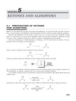
time can be depicted with the sufficient cause diagrammed in Figure 2–1. By sufficient cause we
mean a complete causal mechanism, a minimal set of conditions and events that are sufficient for
the outcome to occur. The circle in the figure comprises five segments, each of which represents a
causal component that must be present or have occured in order for the person to break her hip at that
instant. The first component, labeled A, represents poor weather. The second component, labeled
B, represents an uncleared path for pedestrians. The third component, labeled C, represents a poor
choice of footgear. The fourth component, labeled D, represents the lack of a handrail. The final
component, labeled U, represents all of the other unspecified events, conditions, and characteristics
that must be present or have occured at the instance of the fall that led to a broken hip. For etiologic
effects such as the causation of disease, many and possibly all of the components of a sufficient
cause may be unknown (Rothman, 1976a). We usually include one component cause, labeled U, to
represent the set of unknown factors.
All of the component causes in the sufficient cause are required and must be present or have
occured at the instance of the fall for the person to break a hip. None is superfluous, which means
that blocking the contribution of any component cause prevents the sufficient cause from acting.
For many people, early causal thinking persists in attempts to find single causes as explanations
for observed phenomena. But experience and reasoning show that the causal mechanism for any
effect must consist of a constellation of components that act in concert (Mill, 1862; Mackie, 1965).
In disease etiology, a sufficient cause is a set of conditions sufficient to ensure that the outcome
will occur. Therefore, completing a sufficient cause is tantamount to the onset of disease. Onset
here may refer to the onset of the earliest stage of the disease process or to any transition from one
well-defined and readily characterized stage to the next, such as the onset of signs or symptoms.

A
B
U
C
D

FIGURE 2–1 ● Depiction of the constellation of component
causes that constitute a sufficient cause for hip fracture for a particular
person at a particular time. In the diagram, A represents poor weather,
B represents an uncleared path for pedestrians, C represents a poor
choice of footgear, D represents the lack of a handrail, and U
represents all of the other unspecified events, conditions, and
characteristics that must be present or must have occured at the
instance of the fall that led to a broken hip.


P1: TNL/OVY

P2: SCF/OVY

GRBT241-02

GRBT241-v4.cls

QC: SCF/OVY

Chapter 2

January 28, 2008

●

T1: SCF

Printer: RRD

23:32

Causation and Causal Inference

7

Consider again the role of the handrail in causing hip fracture. The absence of such a handrail
may play a causal role in some sufficient causes but not in others, depending on circumstances such
as the weather, the level of inebriation of the pedestrian, and countless other factors. Our definition
links the lack of a handrail with this one broken hip and does not imply that the lack of this handrail
by itself was sufficient for that hip fracture to occur. With this definition of cause, no specific event,
condition, or characteristic is sufficient by itself to produce disease. The definition does not describe
a complete causal mechanism, but only a component of it. To say that the absence of a handrail is
a component cause of a broken hip does not, however, imply that every person walking down the
path will break a hip. Nor does it imply that if a handrail is installed with properties sufficient to
prevent that broken hip, that no one will break a hip on that same path. There may be other sufficient
causes by which a person could suffer a hip fracture. Each such sufficient cause would be depicted
by its own diagram similar to Figure 2–1. The first of these sufficient causes to be completed by
simultaneous accumulation of all of its component causes will be the one that depicts the mechanism
by which the hip fracture occurs for a particular person. If no sufficient cause is completed while a
person passes along the path, then no hip fracture will occur over the course of that walk.
As noted above, a characteristic of the naive concept of causation is the assumption of a oneto-one correspondence between the observed cause and effect. Under this view, each cause is seen
as “necessary” and “sufficient” in itself to produce the effect, particularly when the cause is an
observable action or event that takes place near in time to the effect. Thus, the flick of a switch

appears to be the singular cause that makes an electric light go on. There are less evident causes,
however, that also operate to produce the effect: a working bulb in the light fixture, intact wiring
from the switch to the bulb, and voltage to produce a current when the circuit is closed. To achieve
the effect of turning on the light, each of these components is as important as moving the switch,
because changing any of these components of the causal constellation will prevent the effect. The
term necessary cause is therefore reserved for a particular type of component cause under the
sufficient-cause model. If any of the component causes appears in every sufficient cause, then that
component cause is called a “necessary” component cause. For the disease to occur, any and all
necessary component causes must be present or must have occurred. For example, one could label
a component cause with the requirement that one must have a hip to suffer a hip fracture. Every
sufficient cause that leads to hip fracture must have that component cause present, because in order
to fracture a hip, one must have a hip to fracture.
The concept of complementary component causes will be useful in applications to epidemiology that follow. For each component cause in a sufficient cause, the set of the other component
causes in that sufficient cause comprises the complementary component causes. For example, in
Figure 2–1, component cause A (poor weather) has as its complementary component causes the
components labeled B, C, D, and U. Component cause B (an uncleared path for pedestrians) has as
its complementary component causes the components labeled A, C, D, and U.

THE NEED FOR A SPECIFIC REFERENCE CONDITION
Component causes must be defined with respect to a clearly specified alternative or reference
condition (often called a referent). Consider again the lack of a handrail along the path. To say that
this condition is a component cause of the broken hip, we have to specify an alternative condition
against which to contrast the cause. The mere presence of a handrail would not suffice. After all,
the hip fracture might still have occurred in the presence of a handrail, if the handrail was too short
or if it was old and made of rotten wood. We might need to specify the presence of a handrail
sufficiently tall and sturdy to break the fall for the absence of that handrail to be a component cause
of the broken hip.
To see the necessity of specifying the alternative event, condition, or characteristic as well as the
causal one, consider an example of a man who took high doses of ibuprofen for several years and
developed a gastric ulcer. Did the man’s use of ibuprofen cause his ulcer? One might at first assume

that the natural contrast would be with what would have happened had he taken nothing instead
of ibuprofen. Given a strong reason to take the ibuprofen, however, that alternative may not make
sense. If the specified alternative to taking ibuprofen is to take acetaminophen, a different drug that
might have been indicated for his problem, and if he would not have developed the ulcer had he used
acetaminophen, then we can say that using ibuprofen caused the ulcer. But ibuprofen did not cause


P1: TNL/OVY

P2: SCF/OVY

GRBT241-02

GRBT241-v4.cls

QC: SCF/OVY
January 28, 2008

T1: SCF

Printer: RRD

23:32

8

Section I

●

Basic Concepts

his ulcer if the specified alternative is taking aspirin and, had he taken aspirin, he still would have
developed the ulcer. The need to specify the alternative to a preventive is illustrated by a newspaper
headline that read: “Rare Meat Cuts Colon Cancer Risk.” Was this a story of an epidemiologic
study comparing the colon cancer rate of a group of people who ate rare red meat with the rate in
a group of vegetarians? No, the study compared persons who ate rare red meat with persons who
ate highly cooked red meat. The same exposure, regular consumption of rare red meat, might have
a preventive effect when contrasted against highly cooked red meat and a causative effect or no
effect in contrast to a vegetarian diet. An event, condition, or characteristic is not a cause by itself
as an intrinsic property it possesses in isolation, but as part of a causal contrast with an alternative
event, condition, or characteristic (Lewis, 1973; Rubin, 1974; Greenland et al., 1999a; Maldonado
and Greenland, 2002; see Chapter 4).

APPLICATION OF THE SUFFICIENT-CAUSE MODEL
TO EPIDEMIOLOGY
The preceding introduction to concepts of sufficient causes and component causes provides the
lexicon for application of the model to epidemiology. For example, tobacco smoking is a cause of
lung cancer, but by itself it is not a sufficient cause, as demonstrated by the fact that most smokers do
not get lung cancer. First, the term smoking is too imprecise to be useful beyond casual description.
One must specify the type of smoke (e.g., cigarette, cigar, pipe, or environmental), whether it is
filtered or unfiltered, the manner and frequency of inhalation, the age at initiation of smoking,
and the duration of smoking. And, however smoking is defined, its alternative needs to be defined
as well. Is it smoking nothing at all, smoking less, smoking something else? Equally important,
even if smoking and its alternative are both defined explicitly, smoking will not cause cancer in
everyone. So who is susceptible to this smoking effect? Or, to put it in other terms, what are the
other components of the causal constellation that act with smoking to produce lung cancer in this
contrast?
Figure 2–2 provides a schematic diagram of three sufficient causes that could be completed
during the follow-up of an individual. The three conditions or events—A, B, and E—have been

defined as binary variables, so they can only take on values of 0 or 1. With the coding of A used
in the figure, its reference level, A = 0, is sometimes causative, but its index level, A = 1, is never
causative. This situation arises because two sufficient causes contain a component cause labeled
“A = 0,” but no sufficient cause contains a component cause labeled “A = 1.” An example of a
condition or event of this sort might be A = 1 for taking a daily multivitamin supplement and
A = 0 for taking no vitamin supplement. With the coding of B and E used in the example depicted
by Figure 2–2, their index levels, B = 1 and E = 1, are sometimes causative, but their reference
levels, B = 0 and C = 0, are never causative. For each variable, the index and reference levels may
represent only two alternative states or events out of many possibilities. Thus, the coding of B might
be B = 1 for smoking 20 cigarettes per day for 40 years and B = 0 for smoking 20 cigarettes per
day for 20 years, followed by 20 years of not smoking. E might be coded E = 1 for living in an
urban neighborhood with low average income and high income inequality, and E = 0 for living in
an urban neighborhood with high average income and low income inequality.
A = 0, B = 1, and E = 1 are individual component causes of the sufficient causes in Figure 2–2.
U1 , U2 , and U3 represent sets of component causes. U1 , for example, is the set of all components
other than A = 0 and B = 1 required to complete the first sufficient cause in Figure 2–2. If we
decided not to specify B = 1, then B = 1 would become part of the set of components that are
causally complementary to A = 0; in other words, B = 1 would then be absorbed into U1 .
Each of the three sufficient causes represented in Figure 2–2 is minimally sufficient to produce
the disease in the individual. That is, only one of these mechanisms needs to be completed for

U1

U2

U3

A=0B=1

A=0E=1

B=1E=1

FIGURE 2–2 ● Three classes of sufficient
causes of a disease (sufficient causes I, II, and III
from left to right).


P1: TNL/OVY

P2: SCF/OVY

GRBT241-02

GRBT241-v4.cls

QC: SCF/OVY

Chapter 2

January 28, 2008

●

T1: SCF

Printer: RRD

23:32

Causation and Causal Inference

9

disease to occur (sufficiency), and there is no superfluous component cause in any mechanism
(minimality)—each component is a required part of that specific causal mechanism. A specific
component cause may play a role in one, several, or all of the causal mechanisms. As noted earlier,
a component cause that appears in all sufficient causes is called a necessary cause of the outcome.
As an example, infection with HIV is a component of every sufficient cause of acquired immune
deficiency syndrome (AIDS) and hence is a necessary cause of AIDS. It has been suggested that
such causes be called “universally necessary,” in recognition that every component of a sufficient
cause is necessary for that sufficient cause (mechanism) to operate (Poole 2001a).
Figure 2–2 does not depict aspects of the causal process such as sequence or timing of action of
the component causes, dose, or other complexities. These can be specified in the description of the
contrast of index and reference conditions that defines each component cause. Thus, if the outcome
is lung cancer and the factor B represents cigarette smoking, it might be defined more explicitly
as smoking at least 20 cigarettes a day of unfiltered cigarettes for at least 40 years beginning at age
20 years or earlier (B = 1), or smoking 20 cigarettes a day of unfiltered cigarettes, beginning at age
20 years or earlier, and then smoking no cigarettes for the next 20 years (B = 0).
In specifying a component cause, the two sides of the causal contrast of which it is composed
should be defined with an eye to realistic choices or options. If prescribing a placebo is not a
realistic therapeutic option, a causal contrast between a new treatment and a placebo in a clinical
trial may be questioned for its dubious relevance to medical practice. In a similar fashion, before
saying that oral contraceptives increase the risk of death over 10 years (e.g., through myocardial
infarction or stroke), we must consider the alternative to taking oral contraceptives. If it involves
getting pregnant, then the risk of death attendant to childbirth might be greater than the risk from
oral contraceptives, making oral contraceptives a preventive rather than a cause. If the alternative
is an equally effective contraceptive without serious side effects, then oral contraceptives may be
described as a cause of death.
To understand prevention in the sufficient-component cause framework, we posit that the alternative condition (in which a component cause is absent) prevents the outcome relative to the

presence of the component cause. Thus, a preventive effect of a factor is represented by specifying
its causative alternative as a component cause. An example is the presence of A = 0 as a component
cause in the first two sufficient causes shown in Figure 2–2. Another example would be to define a
variable, F (not depicted in Fig. 2–2), as “vaccination (F = 1) or no vaccination (F = 0)”. Prevention
of the disease by getting vaccinated (F = 1) would be expressed in the sufficient-component cause
model as causation of the disease by not getting vaccinated (F = 0). This depiction is unproblematic because, once both sides of a causal contrast have been specified, causation and prevention are
merely two sides of the same coin.
Sheps (1958) once asked, “Shall we count the living or the dead?” Death is an event, but
survival is not. Hence, to use the sufficient-component cause model, we must count the dead. This
model restriction can have substantive implications. For instance, some measures and formulas
approximate others only when the outcome is rare. When survival is rare, death is common. In that
case, use of the sufficient-component cause model to inform the analysis will prevent us from taking
advantage of the rare-outcome approximations.
Similarly, etiologies of adverse health outcomes that are conditions or states, but not events, must
be depicted under the sufficient-cause model by reversing the coding of the outcome. Consider spina
bifida, which is the failure of the neural tube to close fully during gestation. There is no point in time
at which spina bifida may be said to have occurred. It would be awkward to define the “incidence
time” of spina bifida as the gestational age at which complete neural tube closure ordinarily occurs.
The sufficient-component cause model would be better suited in this case to defining the event of
complete closure (no spina bifida) as the outcome and to view conditions, events, and characteristics
that prevent this beneficial event as the causes of the adverse condition of spina bifida.

PROBABILITY, RISK, AND CAUSES
In everyday language, “risk” is often used as a synonym for probability. It is also commonly used
as a synonym for “hazard,” as in, “Living near a nuclear power plant is a risk you should avoid.”
Unfortunately, in epidemiologic parlance, even in the scholarly literature, “risk” is frequently used
for many distinct concepts: rate, rate ratio, risk ratio, incidence odds, prevalence, etc. The more


P1: TNL/OVY

P2: SCF/OVY

GRBT241-02

GRBT241-v4.cls

QC: SCF/OVY
January 28, 2008

10

T1: SCF

Printer: RRD

23:32

Section I

●

Basic Concepts

specific, and therefore more useful, definition of risk is “probability of an event during a specified
period of time.”
The term probability has multiple meanings. One is that it is the relative frequency of an event.
Another is that probability is the tendency, or propensity, of an entity to produce an event. A third
meaning is that probability measures someone’s degree of certainty that an event will occur. When
one says “the probability of death in vehicular accidents when traveling >120 km/h is high,” one

means that the proportion of accidents that end with deaths is higher when they involve vehicles
traveling >120 km/h than when they involve vehicles traveling at lower speeds (frequency usage),
that high-speed accidents have a greater tendency than lower-speed accidents to result in deaths
(propensity usage), or that the speaker is more certain that a death will occur in a high-speed accident
than in a lower-speed accident (certainty usage).
The frequency usage of “probability” and “risk,” unlike the propensity and certainty usages,
admits no meaning to the notion of “risk” for an individual beyond the relative frequency of 100%
if the event occurs and 0% if it does not. This restriction of individual risks to 0 or 1 can only be
relaxed to allow values in between by reinterpreting such statements as the frequency with which
the outcome would be seen upon random sampling from a very large population of individuals
deemed to be “like” the individual in some way (e.g., of the same age, sex, and smoking history).
If one accepts this interpretation, whether any actual sampling has been conducted or not, the
notion of individual risk is replaced by the notion of the frequency of the event in question in the
large population from which the individual was sampled. With this view of risk, a risk will change
according to how we group individuals together to evaluate frequencies. Subjective judgment will
inevitably enter into the picture in deciding which characteristics to use for grouping. For instance,
should tomato consumption be taken into account in defining the class of men who are “like” a
given man for purposes of determining his risk of a diagnosis of prostate cancer between his 60th
and 70th birthdays? If so, which study or meta-analysis should be used to factor in this piece of
information?
Unless we have found a set of conditions and events in which the disease does not occur at all,
it is always a reasonable working hypothesis that, no matter how much is known about the etiology
of a disease, some causal components remain unknown. We may be inclined to assign an equal
risk to all individuals whose status for some components is known and identical. We may say, for
example, that men who are heavy cigarette smokers have approximately a 10% lifetime risk of
developing lung cancer. Some interpret this statement to mean that all men would be subject to a
10% probability of lung cancer if they were to become heavy smokers, as if the occurrence of lung
cancer, aside from smoking, were purely a matter of chance. This view is untenable. A probability
may be 10% conditional on one piece of information and higher or lower than 10% if we condition
on other relevant information as well. For instance, men who are heavy cigarette smokers and who

worked for many years in occupations with historically high levels of exposure to airborne asbestos
fibers would be said to have a lifetime lung cancer risk appreciably higher than 10%.
Regardless of whether we interpret probability as relative frequency or degree of certainty, the
assignment of equal risks merely reflects the particular grouping. In our ignorance, the best we can
do in assessing risk is to classify people according to measured risk indicators and then assign the
average risk observed within a class to persons within the class. As knowledge or specification of
additional risk indicators expands, the risk estimates assigned to people will depart from average
according to the presence or absence of other factors that predict the outcome.

STRENGTH OF EFFECTS
The causal model exemplified by Figure 2–2 can facilitate an understanding of some key concepts
such as strength of effect and interaction. As an illustration of strength of effect, Table 2–1 displays
the frequency of the eight possible patterns for exposure to A, B, and E in two hypothetical populations. Now the pie charts in Figure 2–2 depict classes of mechanisms. The first one, for instance,
represents all sufficient causes that, no matter what other component causes they may contain, have
in common the fact that they contain A = 0 and B = 1. The constituents of U1 may, and ordinarily
would, differ from individual to individual. For simplification, we shall suppose, rather unrealistically, that U1 , U2 , and U3 are always present or have always occured for everyone and Figure 2–2
represents all the sufficient causes.


P1: TNL/OVY

P2: SCF/OVY

GRBT241-02

GRBT241-v4.cls

QC: SCF/OVY

T1: SCF

January 28, 2008

Chapter 2

Causation and Causal Inference

●

ˆT A B L E
ˆ

Printer: RRD

23:32

11

ˆ
ˆ

2–1

Exposure Frequencies and Individual Risks in Two Hypothetical Populations
According to the Possible Combinations of the Three Specified Component
Causes in Fig. 2–1
Exposures

Frequency of Exposure Pattern

A

B

E

Sufficient Cause Completed

Risk

Population 1

Population 2

1
1
1
1
0
0
0
0

1
1
0
0
1
1
0

0

1
0
1
0
1
0
1
0

III
None
None
None
I, II, or III
I
II
none

1
0
0
0
1
1
1
0

900

900
100
100
100
100
900
900

100
100
900
900
900
900
100
100

Under these assumptions, the response of each individual to the exposure pattern in a given row
can be found in the response column. The response here is the risk of developing a disease over a
specified time period that is the same for all individuals. For simplification, a deterministic model
of risk is employed, such that individual risks can equal only the value 0 or 1, and no values in
between. A stochastic model of individual risk would relax this restriction and allow individual
risks to lie between 0 and 1.
The proportion getting disease, or incidence proportion, in any subpopulation in Table 2–1 can be
found by summing the number of persons at each exposure pattern with an individual risk of 1 and
dividing this total by the subpopulation size. For example, if exposure A is not considered (e.g., if it
were not measured), the pattern of incidence proportions in population 1 would be those in Table 2–2.
As an example of how the proportions in Table 2–2 were calculated, let us review how the
incidence proportion among persons in population 1 with B = 1 and E = 0 was calculated: There
were 900 persons with A = 1, B = 1, and E = 0, none of whom became cases because there are no

sufficient causes that can culminate in the occurrence of the disease over the study period in persons
with this combination of exposure conditions. (There are two sufficient causes that contain B = 1
as a component cause, but one of them contains the component cause A = 0 and the other contains
the component cause E = 1. The presence of A = 1 or E = 0 blocks these etiologic mechanisms.)
There were 100 persons with A = 0, B = 1, and E = 0, all of whom became cases because they
all had U1 , the set of causal complements for the class of sufficient causes containing A = 0 and

ˆT A B L E
ˆ

ˆ
ˆ

2–2

Incidence Proportions (IP) for Combinations of Component
Causes B and E in Hypothetical Population 1, Assuming That
Component Cause A Is Unmeasured

Cases
Total
IP

B = 1, E = 1

B = 1, E = 0

B = 0, E = 1

B = 0, E = 0

1,000
1,000
1.00

100
1,000
0.10

900
1,000
0.90

0
1,000
0.00


P1: TNL/OVY

P2: SCF/OVY

GRBT241-02

GRBT241-v4.cls

QC: SCF/OVY

T1: SCF

January 28, 2008

Printer: RRD

23:32

12

Section I

ˆT A B L E
ˆ

●

Basic Concepts

ˆ
ˆ

2–3

Incidence Proportions (IP) for Combinations of Component
Causes B and E in Hypothetical Population 2, Assuming That
Component Cause A Is Unmeasured

Cases
Total
IP

B = 1, E = 1

B = 1, E = 0

B = 0, E = 1

B = 0, E = 0

1,000
1,000
1.00

900
1,000
0.90

100
1,000
0.10

0
1,000
0.00

B = 1. Thus, among all 1,000 persons with B = 1 and E = 0, there were 100 cases, for an incidence
proportion of 0.10.
If we were to measure strength of effect by the difference of the incidence proportions, it is
evident from Table 2–2 that for population 1, E = 1 has a much stronger effect than B = 1, because
E = 1 increases the incidence proportion by 0.9 (in both levels of B), whereas B = 1 increases the
incidence proportion by only 0.1 (in both levels of E). Table 2–3 shows the analogous results for

population 2. Although the members of this population have exactly the same causal mechanisms
operating within them as do the members of population 1, the relative strengths of causative factors
E = 1 and B = 1 are reversed, again using the incidence proportion difference as the measure of
strength. B = 1 now has a much stronger effect on the incidence proportion than E = 1, despite
the fact that A, B, and E have no association with one another in either population, and their index
levels (A = 1, B = 1 and E = 1) and reference levels (A = 0, B = 0, and E = 0) are each present
or have occured in exactly half of each population.
The overall difference of incidence proportions contrasting E = 1 with E = 0 is (1,900/2,000) −
(100/2,000) = 0.9 in population 1 and (1,100/2,000) − (900/2,000) = 0.1 in population 2. The
key difference between populations 1 and 2 is the difference in the prevalence of the conditions
under which E = 1 acts to increase risk: that is, the presence of A = 0 or B = 1, but not both.
(When A = 0 and B = 1, E = 1 completes all three sufficient causes in Figure 2–2; it thus does not
increase anyone’s risk, although it may well shorten the time to the outcome.) The prevalence of the
condition, “A = 0 or B = 1 but not both” is 1,800/2,000 = 90% in both levels of E in population 1.
In population 2, this prevalence is only 200/2,000 = 10% in both levels of E. This difference in
the prevalence of the conditions sufficient for E = 1 to increase risk explains the difference in the
strength of the effect of E = 1 as measured by the difference in incidence proportions.
As noted above, the set of all other component causes in all sufficient causes in which a causal
factor participates is called the causal complement of the factor. Thus, A = 0, B = 1, U2 , and U3
make up the causal complement of E = 1 in the above example. This example shows that the strength
of a factor’s effect on the occurrence of a disease in a population, measured as the absolute difference
in incidence proportions, depends on the prevalence of its causal complement. This dependence has
nothing to do with the etiologic mechanism of the component’s action, because the component is
an equal partner in each mechanism in which it appears. Nevertheless, a factor will appear to have
a strong effect, as measured by the difference of proportions getting disease, if its causal complement is common. Conversely, a factor with a rare causal complement will appear to have a weak
effect.
If strength of effect is measured by the ratio of proportions getting disease, as opposed to
the difference, then strength depends on more than a factor’s causal complement. In particular, it
depends additionally on how common or rare the components are of sufficient causes in which the
specified causal factor does not play a role. In this example, given the ubiquity of U1 , the effect of

E = 1 measured in ratio terms depends on the prevalence of E = 1’s causal complement and on the
prevalence of the conjunction of A = 0 and B = 1. If many people have both A = 0 and B = 1,
the “baseline” incidence proportion (i.e., the proportion of not-E or “unexposed” persons getting
disease) will be high and the proportion getting disease due to E will be comparatively low. If few


P1: TNL/OVY

P2: SCF/OVY

GRBT241-02

GRBT241-v4.cls

QC: SCF/OVY

Chapter 2

January 28, 2008

●

T1: SCF

Printer: RRD

23:32

Causation and Causal Inference

13

people have both A = 0 and B = 1, the baseline incidence proportion will be low and the proportion
getting disease due to E = 1 will be comparatively high. Thus, strength of effect measured by the
incidence proportion ratio depends on more conditions than does strength of effect measured by
the incidence proportion difference.
Regardless of how strength of a causal factor’s effect is measured, the public health significance
of that effect does not imply a corresponding degree of etiologic significance. Each component cause
in a given sufficient cause has the same etiologic significance. Given a specific causal mechanism,
any of the component causes can have strong or weak effects using either the difference or ratio
measure. The actual identities of the components of a sufficient cause are part of the mechanics of
causation, whereas the strength of a factor’s effect depends on the time-specific distribution of its
causal complement (if strength is measured in absolute terms) plus the distribution of the components
of all sufficient causes in which the factor does not play a role (if strength is measured in relative
terms). Over a span of time, the strength of the effect of a given factor on disease occurrence may
change because the prevalence of its causal complement in various mechanisms may also change,
even if the causal mechanisms in which the factor and its cofactors act remain unchanged.

INTERACTION AMONG CAUSES
Two component causes acting in the same sufficient cause may be defined as interacting causally
to produce disease. This definition leaves open many possible mechanisms for the interaction,
including those in which two components interact in a direct physical fashion (e.g., two drugs that
react to form a toxic by-product) and those in which one component (the initiator of the pair) alters
a substrate so that the other component (the promoter of the pair) can act. Nonetheless, it excludes
any situation in which one component E is merely a cause of another component F, with no effect
of E on disease except through the component F it causes.
Acting in the same sufficient cause is not the same as one component cause acting to produce a
second component cause, and then the second component going on to produce the disease (Robins
and Greenland 1992, Kaufman et al., 2004). As an example of the distinction, if cigarette smoking
(vs. never smoking) is a component cause of atherosclerosis, and atherosclerosis (vs. no atherosclerosis) causes myocardial infarction, both smoking and atherosclerosis would be component causes

(cofactors) in certain sufficient causes of myocardial infarction. They would not necessarily appear
in the same sufficient cause. Rather, for a sufficient cause involving atherosclerosis as a component
cause, there would be another sufficient cause in which the atherosclerosis component cause was
replaced by all the component causes that brought about the atherosclerosis, including smoking.
Thus, a sequential causal relation between smoking and atherosclerosis would not be enough for
them to interact synergistically in the etiology of myocardial infarction, in the sufficient-cause
sense. Instead, the causal sequence means that smoking can act indirectly, through atherosclerosis,
to bring about myocardial infarction.
Now suppose that, perhaps in addition to the above mechanism, smoking reduces clotting time
and thus causes thrombi that block the coronary arteries if they are narrowed by atherosclerosis. This
mechanism would be represented by a sufficient cause containing both smoking and atherosclerosis
as components and thus would constitute a synergistic interaction between smoking and atherosclerosis in causing myocardial infarction. The presence of this sufficient cause would not, however,
tell us whether smoking also contributed to the myocardial infarction by causing the atherosclerosis. Thus, the basic sufficient-cause model does not alert us to indirect effects (effects of some
component causes mediated by other component causes in the model). Chapters 4 and 12 introduce potential-outcome and graphical models better suited to displaying indirect effects and more
general sequential mechanisms, whereas Chapter 5 discusses in detail interaction as defined in the
potential-outcome framework and its relation to interaction as defined in the sufficient-cause model.

PROPORTION OF DISEASE DUE TO SPECIFIC CAUSES
In Figure 2–2, assuming that the three sufficient causes in the diagram are the only ones operating,
what fraction of disease is caused by E = 1? E = 1 is a component cause of disease in two of the
sufficient-cause mechanisms, II and III, so all disease arising through either of these two mechanisms
is attributable to E = 1. Note that in persons with the exposure pattern A = 0, B = 1, E = 1, all three


P1: TNL/OVY

P2: SCF/OVY

GRBT241-02

GRBT241-v4.cls

14

QC: SCF/OVY
January 28, 2008

T1: SCF

Printer: RRD

23:32

Section I

●

Basic Concepts

sufficient causes would be completed. The first of the three mechanisms to be completed would
be the one that actually produces a given case. If the first one completed is mechanism II or III,
the case would be causally attributable to E = 1. If mechanism I is the first one to be completed,
however, E = 1 would not be part of the sufficient cause producing that case. Without knowing the
completion times of the three mechanisms, among persons with the exposure pattern A = 0, B =
1, E = 1 we cannot tell how many of the 100 cases in population 1 or the 900 cases in population
2 are etiologically attributable to E = 1.
Each of the cases that is etiologically attributable to E = 1 can also be attributed to the other
component causes in the causal mechanisms in which E = 1 acts. Each component cause interacts
with its complementary factors to produce disease, so each case of disease can be attributed to every
component cause in the completed sufficient cause. Note, though, that the attributable fractions

added across component causes of the same disease do not sum to 1, although there is a mistaken
tendency to think that they do. To illustrate the mistake in this tendency, note that a necessary
component cause appears in every completed sufficient cause of disease, and so by itself has an
attributable fraction of 1, without counting the attributable fractions for other component causes.
Because every case of disease can be attributed to every component cause in its causal mechanism,
attributable fractions for different component causes will generally sum to more than 1, and there
is no upper limit for this sum.
A recent debate regarding the proportion of risk factors for coronary heart disease attributable
to particular component causes illustrates the type of errors in inference that can arise when the
sum is thought to be restricted to 1. The debate centers around whether the proportion of coronary
heart disease attributable to high blood cholesterol, high blood pressure, and cigarette smoking
equals 75% or “only 50%” (Magnus and Beaglehole, 2001). If the former, then some have argued
that the search for additional causes would be of limited utility (Beaglehole and Magnus, 2002),
because only 25% of cases “remain to be explained.” By assuming that the proportion explained
by yet unknown component causes cannot exceed 25%, those who support this contention fail to
recognize that cases caused by a sufficient cause that contains any subset of the three named causes
might also contain unknown component causes. Cases stemming from sufficient causes with this
overlapping set of component causes could be prevented by interventions targeting the three named
causes, or by interventions targeting the yet unknown causes when they become known. The latter
interventions could reduce the disease burden by much more than 25%.
As another example, in a cohort of cigarette smokers exposed to arsenic by working in a smelter,
an estimated 75% of the lung cancer rate was attributable to their work environment and an estimated
65% was attributable to their smoking (Pinto et al., 1978; Hertz-Picciotto et al., 1992). There is
no problem with such figures, which merely reflect the multifactorial etiology of disease. So, too,
with coronary heart disease; if 75% of that disease is attributable to high blood cholesterol, high
blood pressure, and cigarette smoking, 100% of it can still be attributable to other causes, known,
suspected, and yet to be discovered. Some of these causes will participate in the same causal
mechanisms as high blood cholesterol, high blood pressure, and cigarette smoking. Beaglehole and
Magnus were correct in thinking that if the three specified component causes combine to explain
75% of cardiovascular disease (CVD) and we somehow eliminated them, there would be only 25%

of CVD cases remaining. But until that 75% is eliminated, any newly discovered component could
cause up to 100% of the CVD we currently have.
The notion that interventions targeting high blood cholesterol, high blood pressure, and cigarette
smoking could eliminate 75% of coronary heart disease is unrealistic given currently available
intervention strategies. Although progress can be made to reduce the effect of these risk factors, it
is unlikely that any of them could be completely eradicated from any large population in the near
term. Estimates of the public health effect of eliminating diseases themselves as causes of death
(Murray et al., 2002) are even further removed from reality, because they fail to account for all the
effects of interventions required to achieve the disease elimination, including unanticipated side
effects (Greenland, 2002a, 2005a).
The debate about coronary heart disease attribution to component causes is reminiscent of an
earlier debate regarding causes of cancer. In their widely cited work, The Causes of Cancer, Doll and
Peto (1981, Table 20) created a table giving their estimates of the fraction of all cancers caused by
various agents. The fractions summed to nearly 100%. Although the authors acknowledged that any
case could be caused by more than one agent (which means that, given enough agents, the attributable


P1: TNL/OVY

P2: SCF/OVY

GRBT241-02

GRBT241-v4.cls

QC: SCF/OVY

Chapter 2

January 28, 2008

●

T1: SCF

Printer: RRD

23:32

Causation and Causal Inference

15

fractions would sum to far more than 100%), they referred to this situation as a “difficulty” and
an “anomaly” that they chose to ignore. Subsequently, one of the authors acknowledged that the
attributable fraction could sum to greater than 100% (Peto, 1985). It is neither a difficulty nor an
anomaly nor something we can safely ignore, but simply a consequence of the fact that no event
has a single agent as the cause. The fraction of disease that can be attributed to known causes will
grow without bound as more causes are discovered. Only the fraction of disease attributable to a
single component cause cannot exceed 100%.
In a similar vein, much publicity attended the pronouncement in 1960 that as much as 90%
of cancer is environmentally caused (Higginson, 1960). Here, “environment” was thought of as
representing all nongenetic component causes, and thus included not only the physical environment,
but also the social environment and all individual human behavior that is not genetically determined.
Hence, environmental component causes must be present to some extent in every sufficient cause
of a disease. Thus, Higginson’s estimate of 90% was an underestimate.
One can also show that 100% of any disease is inherited, even when environmental factors are
component causes. MacMahon (1968) cited the example given by Hogben (1933) of yellow shanks,
a trait occurring in certain genetic strains of fowl fed on yellow corn. Both a particular set of genes
and a yellow-corn diet are necessary to produce yellow shanks. A farmer with several strains of

fowl who feeds them all only yellow corn would consider yellow shanks to be a genetic condition,
because only one strain would get yellow shanks, despite all strains getting the same diet. A different
farmer who owned only the strain liable to get yellow shanks but who fed some of the birds yellow
corn and others white corn would consider yellow shanks to be an environmentally determined
condition because it depends on diet. In humans, the mental retardation caused by phenylketonuria
is considered by many to be purely genetic. This retardation can, however, be successfully prevented
by dietary intervention, which demonstrates the presence of an environmental cause. In reality,
yellow shanks, phenylketonuria, and other diseases and conditions are determined by an interaction
of genes and environment. It makes no sense to allocate a portion of the causation to either genes
or environment separately when both may act together in sufficient causes.
Nonetheless, many researchers have compared disease occurrence in identical and nonidentical
twins to estimate the fraction of disease that is inherited. These twin-study and other heritability
indices assess only the relative role of environmental and genetic causes of disease in a particular
setting. For example, some genetic causes may be necessary components of every causal mechanism.
If everyone in a population has an identical set of the genes that cause disease, however, their effect
is not included in heritability indices, despite the fact that the genes are causes of the disease.
The two farmers in the preceding example would offer very different values for the heritability
of yellow shanks, despite the fact that the condition is always 100% dependent on having certain
genes.
Every case of every disease has some environmental and some genetic component causes, and
therefore every case can be attributed both to genes and to environment. No paradox exists as long
as it is understood that the fractions of disease attributable to genes and to environment overlap
with one another. Thus, debates over what proportion of all occurrences of a disease are genetic
and what proportion are environmental, inasmuch as these debates assume that the shares must add
up to 100%, are fallacious and distracting from more worthwhile pursuits.
On an even more general level, the question of whether a given disease does or does not have
a “multifactorial etiology” can be answered once and for all in the affirmative. All diseases have
multifactorial etiologies. It is therefore completely unremarkable for a given disease to have such
an etiology, and no time or money should be spent on research trying to answer the question of
whether a particular disease does or does not have a multifactorial etiology. They all do. The job of

etiologic research is to identify components of those etiologies.

INDUCTION PERIOD
Pie-chart diagrams of sufficient causes and their components such as those in Figure 2–2 are not
well suited to provide a model for conceptualizing the induction period, which may be defined as
the period of time from causal action until disease initiation. There is no way to tell from a piechart diagram of a sufficient cause which components affect each other, which components must
come before or after others, for which components the temporal order is irrelevant, etc. The crucial