mật mã va an ninh mạng nguyễn đức thái bp orig sinhvienzone com
Bạn đang xem bản rút gọn của tài liệu. Xem và tải ngay bản đầy đủ của tài liệu tại đây (698.82 KB, 82 trang )
⑥✇✁✂✄☎✆✝✞✟✡☛☞✌✍✏✑✒✓✔✕✖✗✘✙✚✤✥✦✧★✩✪✫✬✭✮✰✱✲✳✴✵✶✷✸✹✺❁②❆⑤
M ASARYK U NIVERSITY
FACULTY OF I NFORMATICS
Coding theory, cryptography and
cryptographic protocols – exercises
with solutions
(given in 2006)
B ACHELOR THESIS
Zuzana Kuklov´a
Brno, Spring 2007
SinhVienZone.com
/>
Declaration
Hereby I declare, that this paper is my original authorial work, which I have worked out by
my own. All sources, references and literature used or excerpted during elaboration of this
work are properly cited and listed in complete reference to the due source.
Advisor: prof. RNDr. Jozef Gruska, DrSc.
ii
SinhVienZone.com
/>
Acknowledgement
I would like to thank prof. RNDr. Jozef Gruska, DrSc. and Mgr. Luk´asˇ Boh´acˇ for their inspiring comments which have essentially contributed to fulfilling of the presented work.
I am obliged to my family for understanding and furtherance.
iii
SinhVienZone.com
/>
Abstract
The main goal of this work is to present detailed solutions of exercises that have been submitted to students of the course Coding, cryptography and cryptographic protocols, given
by prof. RNDr. Jozef Gruska, DrSc. in 2006 as homeworks. This way a handbook of solved
exercises from coding theory and cryptography is created. Ahead of each set of new exercises we include main concepts and results from the corresponding lecture that are needed
to solve exercises.
iv
SinhVienZone.com
/>
Keywords
Coding theory, code, linear code, cyclic code, cryptography, cryptosystem, cryptoanalysis,
secret key cryptography, public key cryptography, digital signature, subliminal channel, elliptic curve, factorization, prime recognition, identification, authentication, bit commitment,
zero knowledge proof
v
SinhVienZone.com
/>
Contents
Introduction . . . . . . . . . . . . . . . . . . . . . . . . . . . . . .
1 Basics of Coding Theory . . . . . . . . . . . . . . . . . . . . .
1.1 Definition of Code . . . . . . . . . . . . . . . . . . . . .
1.2 Equivalence of Codes . . . . . . . . . . . . . . . . . . . .
1.3 Properties of Code . . . . . . . . . . . . . . . . . . . . .
1.4 Entropy . . . . . . . . . . . . . . . . . . . . . . . . . . . .
1.5 Exercises . . . . . . . . . . . . . . . . . . . . . . . . . . .
2 Linear Codes . . . . . . . . . . . . . . . . . . . . . . . . . . .
2.1 Definition of Linear Code . . . . . . . . . . . . . . . . .
2.2 Equivalence of Linear Codes . . . . . . . . . . . . . . . .
2.3 Dual Code . . . . . . . . . . . . . . . . . . . . . . . . . .
2.4 Encoding with Linear Codes . . . . . . . . . . . . . . . .
2.5 Decoding of Linear Codes . . . . . . . . . . . . . . . . .
2.6 Hamming Code . . . . . . . . . . . . . . . . . . . . . . .
2.7 Properties of Linear Code . . . . . . . . . . . . . . . . .
2.8 Exercises . . . . . . . . . . . . . . . . . . . . . . . . . . .
3 Cyclic Codes . . . . . . . . . . . . . . . . . . . . . . . . . . . .
3.1 Definition of Cyclic Code . . . . . . . . . . . . . . . . . .
3.2 Algebraic Characterization of Cyclic Codes . . . . . . .
3.3 Generator Matrix, Parity Check Matrix and Dual Code
3.4 Encoding with Cyclic Codes . . . . . . . . . . . . . . . .
3.5 Hamming Code . . . . . . . . . . . . . . . . . . . . . . .
3.6 Exercises . . . . . . . . . . . . . . . . . . . . . . . . . . .
4 Secret Key Cryptography . . . . . . . . . . . . . . . . . . . .
4.1 Cryptosystem . . . . . . . . . . . . . . . . . . . . . . . .
4.2 Cryptoanalysis . . . . . . . . . . . . . . . . . . . . . . .
4.3 Secret Key Cryptosystem . . . . . . . . . . . . . . . . . .
4.3.1 Caesar Cryptosystem . . . . . . . . . . . . . . . .
4.3.2 Polybious Cryptosystem . . . . . . . . . . . . . .
4.3.3 Hill Cryptosystem . . . . . . . . . . . . . . . . .
4.3.4 Affine Cryptosystem . . . . . . . . . . . . . . . .
4.3.5 Playfair Cryptosystem . . . . . . . . . . . . . . .
4.3.6 Vigenere and Autoclave Cryptosystems . . . . .
4.3.7 One time pad Cryptosystem . . . . . . . . . . .
4.4 Perfect Secret Cryptosystem . . . . . . . . . . . . . . . .
4.5 Exercises . . . . . . . . . . . . . . . . . . . . . . . . . . .
5 Public Key Cryptography . . . . . . . . . . . . . . . . . . . .
5.1 Diffie-Hellman Key Exchange . . . . . . . . . . . . . . .
5.2 Blom’s Key Predistribution Protocol . . . . . . . . . . .
.
.
.
.
.
.
.
.
.
.
.
.
.
.
.
.
.
.
.
.
.
.
.
.
.
.
.
.
.
.
.
.
.
.
.
.
.
.
.
.
.
.
.
.
.
.
.
.
.
.
.
.
.
.
.
.
.
.
.
.
.
.
.
.
.
.
.
.
.
.
.
.
.
.
.
.
.
.
.
.
.
.
.
.
.
.
.
.
.
.
.
.
.
.
.
.
.
.
.
.
.
.
.
.
.
.
.
.
.
.
.
.
.
.
.
.
.
.
.
.
.
.
.
.
.
.
.
.
.
.
.
.
.
.
.
.
.
.
.
.
.
.
.
.
.
.
.
.
.
.
.
.
.
.
.
.
.
.
.
.
.
.
.
.
.
.
.
.
.
.
.
.
.
.
.
.
.
.
.
.
.
.
.
.
.
.
.
.
.
.
.
.
.
.
.
.
.
.
.
.
.
.
.
.
.
.
.
.
.
.
.
.
.
.
.
.
.
.
.
.
.
.
.
.
.
.
.
.
.
.
.
.
.
.
.
.
.
.
.
.
.
.
.
.
.
.
.
.
.
.
.
.
.
.
.
.
.
.
.
.
.
.
.
.
.
.
.
.
.
.
.
.
.
.
.
.
.
.
.
.
.
.
.
.
.
.
.
.
.
.
.
.
.
.
.
.
.
.
.
.
.
.
.
.
.
.
.
.
.
.
.
.
.
.
.
.
.
.
.
.
.
.
.
.
.
.
.
.
.
.
.
.
.
.
.
.
.
.
.
.
.
.
.
.
.
.
.
.
.
.
.
.
.
.
.
.
.
.
.
.
.
.
.
.
.
.
.
.
.
.
.
.
.
.
.
.
.
.
.
.
.
.
.
.
.
.
.
.
.
.
.
.
.
.
.
.
.
.
.
.
.
.
.
.
.
.
.
.
.
.
.
.
.
.
.
.
.
.
.
.
.
.
.
.
.
.
.
.
.
.
.
.
.
.
.
.
.
.
.
.
.
.
.
.
.
.
.
.
.
.
.
.
.
.
.
.
.
.
.
.
.
.
.
.
.
.
.
.
.
.
.
.
.
.
.
.
.
.
.
.
.
.
.
.
.
.
.
.
.
.
.
.
.
.
.
.
.
.
.
.
.
.
.
.
.
.
.
3
4
4
4
5
5
6
12
12
13
13
13
14
14
15
15
22
22
22
23
24
24
24
30
30
30
31
32
32
32
32
32
33
33
33
33
39
39
39
1
SinhVienZone.com
/>
5.3 Cryptography and Computational Complexity . . . . . . . .
5.4 RSA Cryptosystem . . . . . . . . . . . . . . . . . . . . . . . .
5.5 Rabin-Miller’s Prime Recognition . . . . . . . . . . . . . . . .
5.6 Exercises . . . . . . . . . . . . . . . . . . . . . . . . . . . . . .
6 Other Public Key Cryptosystems . . . . . . . . . . . . . . . . . . .
6.1 Rabin Cryptosystem . . . . . . . . . . . . . . . . . . . . . . .
6.2 ElGamal Cryptosystem . . . . . . . . . . . . . . . . . . . . . .
6.3 Exercises . . . . . . . . . . . . . . . . . . . . . . . . . . . . . .
7 Digital Signature . . . . . . . . . . . . . . . . . . . . . . . . . . . .
7.1 Digital Signature Scheme . . . . . . . . . . . . . . . . . . . . .
7.2 Attacks on Digital Signature . . . . . . . . . . . . . . . . . . .
7.3 RSA Signatures . . . . . . . . . . . . . . . . . . . . . . . . . .
7.4 ElGamal Signatures . . . . . . . . . . . . . . . . . . . . . . . .
7.5 Digital Signature Algorithm . . . . . . . . . . . . . . . . . . .
7.6 Ong-Schnorr-Shamir Subliminal Channel Scheme . . . . . .
7.7 Lamport Signature Scheme . . . . . . . . . . . . . . . . . . .
7.8 Exercises . . . . . . . . . . . . . . . . . . . . . . . . . . . . . .
8 Elliptic Curve Cryptography and Factorization . . . . . . . . . .
8.1 Elliptic Curve . . . . . . . . . . . . . . . . . . . . . . . . . . .
8.2 Addition of Points . . . . . . . . . . . . . . . . . . . . . . . . .
8.3 Elliptic Curves over a Finite Field . . . . . . . . . . . . . . . .
8.4 Discrete Logarithm Problem for Elliptic Curves . . . . . . . .
8.5 Factorization . . . . . . . . . . . . . . . . . . . . . . . . . . . .
8.5.1 Factorization with Elliptic Curves . . . . . . . . . . .
8.5.2 Pollard’s Rho Method . . . . . . . . . . . . . . . . . .
8.6 Exercises . . . . . . . . . . . . . . . . . . . . . . . . . . . . . .
9 User Identification, Message Authentication and Secret Sharing
9.1 User Identification . . . . . . . . . . . . . . . . . . . . . . . .
9.2 Message Authentication . . . . . . . . . . . . . . . . . . . . .
9.3 Secret Sharing Scheme . . . . . . . . . . . . . . . . . . . . . .
9.3.1 Shamir’s (n, t)-secret sharing scheme . . . . . . . . .
9.4 Exercises . . . . . . . . . . . . . . . . . . . . . . . . . . . . . .
10 Bit Commitment Protocols and Zero Knowledge Proofs . . . . .
10.1 Bit Commitment Protocols . . . . . . . . . . . . . . . . . . . .
10.2 Oblivious Transfer Problem . . . . . . . . . . . . . . . . . . .
10.3 Zero Knowledge Proof Protocols . . . . . . . . . . . . . . . .
10.4 3-Colorability of Graphs . . . . . . . . . . . . . . . . . . . . .
10.5 Exercises . . . . . . . . . . . . . . . . . . . . . . . . . . . . . .
Bibliography . . . . . . . . . . . . . . . . . . . . . . . . . . . . . . . .
.
.
.
.
.
.
.
.
.
.
.
.
.
.
.
.
.
.
.
.
.
.
.
.
.
.
.
.
.
.
.
.
.
.
.
.
.
.
.
.
.
.
.
.
.
.
.
.
.
.
.
.
.
.
.
.
.
.
.
.
.
.
.
.
.
.
.
.
.
.
.
.
.
.
.
.
.
.
.
.
.
.
.
.
.
.
.
.
.
.
.
.
.
.
.
.
.
.
.
.
.
.
.
.
.
.
.
.
.
.
.
.
.
.
.
.
.
.
.
.
.
.
.
.
.
.
.
.
.
.
.
.
.
.
.
.
.
.
.
.
.
.
.
.
.
.
.
.
.
.
.
.
.
.
.
.
.
.
.
.
.
.
.
.
.
.
.
.
.
.
.
.
.
.
.
.
.
.
.
.
.
.
.
.
.
.
.
.
.
.
.
.
.
.
.
.
.
.
.
.
.
.
.
.
.
.
.
.
.
.
.
.
.
.
.
.
.
.
.
.
.
.
.
.
.
.
.
.
.
.
.
.
.
.
.
.
.
.
.
.
.
.
.
.
.
.
.
.
.
.
.
.
.
.
.
.
.
.
.
.
.
.
.
.
.
.
.
.
.
.
.
.
.
.
.
.
.
.
.
.
.
.
.
.
.
.
.
.
.
.
.
.
.
.
.
.
.
.
.
.
.
.
.
.
.
.
.
.
.
.
.
.
.
.
.
.
.
.
.
.
.
.
.
.
.
.
.
.
.
.
.
.
.
.
.
.
.
.
.
.
.
.
.
.
.
.
.
.
.
.
.
.
.
.
.
.
.
.
.
.
.
.
.
.
.
.
.
.
.
.
.
.
.
.
.
.
.
.
.
.
.
.
.
.
.
.
.
.
.
.
40
40
40
41
45
45
45
45
49
49
49
50
50
50
51
51
51
56
56
56
57
57
57
57
57
58
64
64
65
65
65
66
70
70
70
71
71
72
76
2
SinhVienZone.com
/>
Introduction
The main goal of this work is to present detailed solutions of exercises that have been submitted to students of the course Coding, cryptography and cryptographic protocols, given
by prof. RNDr. Jozef Gruska, DrSc. in 2006 as homeworks. The authors of exercises are Mgr.
ˇ
Luk´asˇ Boh´acˇ , RNDr. Jan Bouda, Ph.D., Mgr. Ivan Fial´ık and Mgr. Josef Sprojcar.
This way we create a handbook of solved exercises from coding theory and cryptography
that could be useful to the future students of the above course. Ahead of each set of exercises
we include main concepts and results from the corresponding lecture that are needed to
solve exercises. The main source of solutions presented here are solutions submitted by the
students of the above course. The solutions were adopted and/or modified to achieve a
uniform presentation of the exercises and of their solutions.
For some of the exercises we present not only one, but several solutions in the case sufficiently different approaches have been used in the submitted solutions. Some of the solutions are newly created. The authors of solutions are cited. The solutions, where no author is
stated, were created or submitted by myself.
Ciphers and codes have been a part of human history since the time of Egyptian pharaohs.
They arose from the requirement to protect secrets and messages against aliens and enemies.
People were trying to protect their own secrets, as hard as they were trying to discover secrets of others. Their competition led up to invent better and better ciphers and codes that
cannot be so easily broken through. And this is how the cryptography progresses till now:
code makers are inventing new more sophisticated and secure ciphers and codes and code
breakers try to crack them. The struggle between the code makers and the code breakers
stood in the background of various historical events – it decided battles, revolts and human
lives.
Today, encipherment, coding and authentication are an inseparable part of our daily life.
Therefore, it is very important to know the history of ciphers, how they work and where
are their weaknesses. The basics can be obtained in the course Coding, Cryptography and
Cryptographic Protocols, taught at the Faculty of Informatics every year by prof. RNDr. Jozef
Gruska, DrSc.
The bibliography I used as a source of information for my work and which can be useful
for everyone interested in more detailed information about studied problems is listed at the
end of the work. Simultaneously, there are listed some interesting web pages, where can be
found more about problems, as well as some useful tools for solving exercises.
3
SinhVienZone.com
/>
Chapter 1
Basics of Coding Theory
Coding theory has developed methods of protecting information against noise. Without coding theory and error correcting codes, there would be no deep space pictures, no satellite TV,
no CD, no DVD and many more. . .
1.1
Definition of Code
A code C over an alphabet Σ is a subset of Σ∗ (C ⊆ Σ∗ ). A q-ary code is a code over alphabet
of q symbols. A binary code is a code over the alphabet {0, 1}.
The Hamming distance h(x, y) of words x, y is the number of positions, where words x
and y differs. The properties of Hamming distance are following:
1.
h(x, y) = 0 ⇔ x = y
2.
h(x, y) = h(y, x)
3.
h(x, z) ≤ h(x, y) + h(y, z)
An important parameter of codes is their minimal distance h(C).
h(C) = min{h(x, y)|x, y ∈ C, x = y},
h(C) is the smallest number of bits needed to change one codeword into another. Code C
can detect up to s errors if h(C) ≥ s + 1. Code C can correct up to t errors if h(C) ≥ 2t + 1.
An (n, M, d)-code C is a code such that n is the length of codewords, M is the number of
codewords and d is the minimum distance of C. A good (n, M, d) code has small n and large
M and d.
The main coding problem is to optimize one of the parameters n, M , d for given values
of the other two. Aq (n, d) is the largest M such that there is a q-ary (n, M, d)-code. It holds
that
1.
Aq (n, 1) = q n
2.
Aq (n, n) = q
1.2
Equivalence of Codes
Two q-ary codes are equivalent if one can be obtained from the other by a combination of
following operations:
1.
permutation of the positions of the code;
4
SinhVienZone.com
/>
1. B ASICS OF C ODING T HEORY
2.
permutation of symbols at the fixed positions.
Any q-ary (n, M, d)-code is equivalent to an (n, M, d)-code which contains the zero codeword.
If d is odd then a binary (n, M, d)-code exists if and only if a binary (n + 1, M, d + 1)-code
exists. That means that if d is odd then A2 (n, d) = A2 (n + 1, d + 1) and if d is even then
A2 (n, d) = A2 (n − 1, d − 1).
1.3
Properties of Code
Fqn is a set of all words of length n over alphabet {0, 1, . . . q − 1}. For any codeword u ∈ Fqn
and any integer r ≥ 0 the sphere of radius r and center u is defined as
S(u, r) = {v ∈ Fqn |d(u, v) ≤ r}.
A sphere of radius r in Fqn , 0 ≤ r ≤ n contains
r
i=0
n
(q − 1)i
i
words.
The sphere packing bound: If C is a q-ary (n, M, 2t + 1)-code, then
t
M·
i=0
n
(q − 1)i ≤ q n .
i
(1.1)
A code which achieves the sphere packing bound (a code that satisfies the equality) is called
a perfect code.
Singleton’s bound: If C is a q-ary (n, M, d)-code, then
M ≤ q n−d+1 .
(1.2)
Gilbert-Varshamov’s bound (lower bound): For a given d ≤ n, there exists a q-ary
(n, M, d)-code with
qn
M ≥ d−1 n
(1.3)
j
(q
−
1)
j=0 j
and therefore
Aq (n, d) ≥
1.4
qn
d−1 n
j=0 j
(q − 1)j
.
Entropy
Let X be a random variable (source) which takes a value x with probability p(x). The entropy
of X is defined by
S(X) = −
p(x) lg p(x)
(1.4)
x
and it is considered to be the information content of X. Shannon’s noiseless coding theorem
says that in order to transmit n values of X we need to use nS(X) bits. More exactly, we
cannot do better and we should reach the bound nS(X) as close as possible.
5
SinhVienZone.com
/>
1. B ASICS OF C ODING T HEORY
1.5
Exercises
Exercise
1.1
Determine Aq (n, d) and write or describe the corresponding code that achieves the upper
bound.
1.
A2 (8, d) for d = 1 and d = 2.
2.
A2 (n, 4) for n = 4, n = 5 and n = 6.
3.
Aq (4, 3) for q = 2 and q = 3.
Solution
1.
1.1.1
A2 (8, d)
(a)
d = 1. A2 (8, 1) = 28 . Code C contains all binary words of the length eight.
(b) d = 2. A2 (8, 2) = A2 (7, 1) = 27 . Code C contains all binary words of the length
seven with the parity bit added.
2.
A2 (n, 4)
(a)
n = 4. A2 (4, 4) = 2. C = {0000, 1111}.
(b) n = 5. A2 (5, 4) = 2 because C contains the word 00000, then it can contain only
one word with four or five ones. C cannot contain any other word because of the
given minimum distance d = 4.
(c)
3.
n = 6. A2 (6, 4) = A2 (5, 3). We know from the first lesson, that A2 (5, 3) = 4 and
one of the corresponding codes is the code C3 = {00000, 01101, 10110, 11011}.
(6, 4, 4)-codes exist and come from the code C3 . There is, for example, the code
C = {000000, 011011, 101101, 110110} (it is the code C3 with a parity bit added).
Aq (4, 3)
(a)
q = 2. A2 (4, 3) = 2. Indeed, because 0000 ∈ C, there is no word in C with less
then three ones and there can be only one word with three or four ones in C. One
of A2 (4, 3)-codes is code C = {0000, 0111}.
(b) q = 3. A3 (4, 3) ≤ q n−d+1 = 32 according to Singleton’s bound. And we can find
a ternary (4, 9, 3)-code C = {0000, 0111, 0222, 1012, 1120, 1201, 2021, 2102, 2210}
that reaches the Singleton’s bound (1.2).
Exercise
1.2
Let q > 1. What is the relation (≤, ≥ or =) between
1.
Aq (2n, d) and Aq (n, d)
2.
Aq (n, d) and Aq (n + 2, 2d)
3.
A2 (n, 2d − 1) and A2 (n + 1, 2d)
6
SinhVienZone.com
/>
1. B ASICS OF C ODING T HEORY
Solution
1.
1.2.1
Aq (2n, d) ≥ Aq (n, d)
Let Aq (2n, d) = M1 and Aq (n, d) = M2 . We need to show that for each q, n and d it holds
M1 ≥ M2 . To do that, we need to determine which code contains more codewords. We
compute it using the Singleton bound (1.2), page 5:
M1 ≤ q 2n−d+1 ,
M2 ≤ q n−d+1 .
We can see that
q 2n−d+1 = q n q n−d+1 ≥ q n−d+1
and therefore Aq (2n, d) contains q n codewords more then Aq (n, d) and hence Aq (2n, d) ≥
Aq (n, d).
We can see that if we have two codes of different length with the same minimum distance, the code with longer codewords contains more codewords then the other code.
2.
Aq (n, d) and Aq (n + 2, 2d) are incomparable as we can see in the following examples:
if q = 2, n = 2 and d = 1 then A2 (2, 1) = 22 < A2 (4, 2) = A2 (3, 1) = 23 ,
if n = 2 and d = 2 then Aq (2, 2) = q = Aq (4, 4) = q,
if q = 2, n = 4 and d = 2 then A2 (4, 2) = A2 (3, 1) = 23 > A2 (6, 4) = A2 (5, 3) = 4.
3.
A2 (n, 2d − 1) = A2 (n + 1, 2d) Because
2d − 1 is odd, we have A2 (n, 2d − 1) = A2 (n + 1, (2d − 1) + 1) = A2 (n + 1, 2d).
Exercise
1.3
Consider the binary erasure channel which has two inputs (0 or 1) and three outputs (0, 1
or ?). The symbol is correctly received with probability 1 − p and erased with probability p.
Erasure is indicated by receiving the symbol ’?’.
1.
Consider the nearest neighbour decoding strategy and the code
C = {011, 101, 110, 000}.
Calculate the probability that the received word is decoded incorrectly and the probability of error detection.
2.
Consider a code C with the minimum distance h(C) = d. How many erasures can the
code C detect and correct?
3.
Consider a binary channel that has both erasures and errors. Give the lower bound for
the minimum Hamming distance for a code capable of correcting all combinations of
e erasures and t errors.
7
SinhVienZone.com
/>
1. B ASICS OF C ODING T HEORY
Solution
1.
1.3.1
The received word is decoded incorrectly only if it contains two or more question
marks. The probability of an erroneous decoding is:
3 · p2 (1 − p) + p3 = 3p2 − 3p3 + p3 = 3p2 − 2p3
We can detect every erasure because the question mark is not an element of the code
alphabet. And we can correct one erasure in the codeword. So the probability that the
received word is decoded correctly is:
(1−p)3 +3·p·(1−p)2 = 1−3p+3p2 −p3 +3p−6p2 +3p3 = 1−3p2 +2p3 = 1−(3p2 −2p3 )
2.
Code C can detect every erasure – in this case we receive a symbol that cannot be sent.
Code C can correct up to d − 1 erasures in a codeword. When receiving a word with
e ≤ d − 1 erased symbols, we delete positions where we received a question mark
in all codewords of C. This way we get a new code C . The length of the codewords
decreases from n to n − e and the d(C) decreases to d − e ≥ 1. That means, that there
is still the Hamming distance h(x, y) ≥ 1 of each two words x, y of the code C . So we
can decode the received word correctly.
3.
The minimum distance for a code C capable of correcting all combinations of e erasures
and t errors is d(C) = 2t + e + 1. When there are some (less then or equal to e) erased
symbols, we transform the code C to code C the same way as it was described above
and d(C ) ≥ 2t + 1. According to the definition of Hamming distance, we can correct
up to t errors in the codeword.
Exercise
1.4
You are given two dices with 6 faces. Design a binary Huffman code for encoding the sum
of two dices. Compare efficiency of the proposed code with Shannon’s entropy.
Solution
1.4.1
All the possible sums of two dices and their probabilities are written in the Table 1.1.
At the Figure 1.1 there you can see how to design a Huffman code for the given data. (For
short, there is written 1 there instead of 1/36 and so on.)
In the Table 1.2, there are written the possible values and their codes. We can see, that it
is a prefix code.
We calculate the Shannon’s entropy (1.4) as follows:
S(X) = −
p(x) · lg p(x) ≈ 3.2744
x
By Shannon’s theorem, we need 3.2744 bits in average per message. Now, we calculate the
efficiency E of our code:
p(x)|code(x)| = 3 ·
E=
x
2+3+2
1+1
3+4+5+6+5+4
+4·
+5·
≈ 3.3056
36
36
36
By using our code we need circa 0.03 bits per message (sum of two dices) more.
8
SinhVienZone.com
/>
1. B ASICS OF C ODING T HEORY
x
2
3
4
5
6
7
8
9
10
11
12
p(x)
1/36
2/36
3/36
4/36
5/36
6/36
5/36
4/36
3/36
2/36
1/36
Table 1.1: Messages and their probabilities
Figure 1.1: Design of the Huffman code
Σ
2
3
4
5
6
7
8
9
10
11
12
code
00101
1000
000
011
110
111
101
010
1001
0011
00100
Table 1.2: Messages and their codes
9
SinhVienZone.com
/>
1. B ASICS OF C ODING T HEORY
Exercise
1.5
You have found the belt with an ornament displayed at the Figure 1.2. It seems that the
ornament is related to coding theory. Decode the hidden message.
Figure 1.2: Ornament belt
Solution
1.5.1 by Luk´asˇ Boh´acˇ
NRZI (Non Return to Zero, Inverted) signal encoding was used. A change of the level encodes 1, staying on the level encodes 0. The bit-string encodes the message CODE NRZI (8bit
ASCII code) as you can see at the Figure 1.3.
Figure 1.3: Ornament belt – the hidden message
Exercise
1.6
A single character was encoded into the following long message. Decode.
012221102011200210110121222012001211122201
Solution
1.6.1
The message is 42 bits long and there should be hidden only one single character. Therefore
there is a strong probability that it is a graphic cipher. Our task is to form the message into
a table and look for the hidden letter. The character is formed by twos when we put the
message into a table with six rows and seven columns. And here we can see the letter G:
10
SinhVienZone.com
/>
1. B ASICS OF C ODING T HEORY
0
0
0
1
1
1
1
2
2
2
2
1
2
0
1
1
0
2
2
1
0
2
0
2
2
1
1
2
1
2
1
2
1
2
2
0
1
0
0
0
1
1
The letter G is better to see when replacing the 1s and 0s by spaces:
2
2
2
2
2
2
2
2
2
2
2
2
2
2
2
11
SinhVienZone.com
/>
Chapter 2
Linear Codes
Linear codes are important because they have very concise description, very nice properties,
very easy encoding and in principle quite easy decoding.
2.1
Definition of Linear Code
Linear codes are special sets of words of length n over an alphabet {0, . . . , q − 1} where q is
a power of prime.
A subset C ⊆ V (n, q) is called a linear code if
1.
for all u, v ∈ C: u + v ∈ C;
2.
for all u ∈ C, a ∈ GF (q): au ∈ C,
where GF (q) is Galois field, the set {0, . . . , q − 1} with operations + and · taken modulo q,
where q is a prime.
We can also say that a subset C ⊆ V (n, q) is a linear code if one of the following conditions
are satisfied:
1.
C is a subspace of V (n, q);
2.
sum of any two codewords from C is in C (for the case q = 2).
If C is a k-dimensional subspace of V (n, q) then C is called [n, k]-code and C consists of
q k codewords.
If S is a set of vectors of a vector space then S is the set of all linear combinations of
vectors from S. For any subset S of a vector space the set S is a linear space that consists of
the following words:
•
the zero word;
•
all words from S;
•
all sums of two or more words from S.
The weight of a codeword x denoted as w(x) is the number of nonzero entries of x. If
x, y ∈ V (n, q) then the Hamming distance h(x, y) = w(x − y). If C is a linear code then
the weight of code C, denoted as w(C), is the smallest weight of all the weights of nonzero
codewords from C and w(C) = h(C).
If C is a linear [n, k]-code then it has a basis of k codewords.
A k × n matrix whose rows forms a basis of a linear [n, k]-code (subspace) C is said to be
a generator matrix of C.
12
SinhVienZone.com
/>
2. L INEAR C ODES
2.2
Equivalence of Linear Codes
Two linear codes over GF (q) are equivalent if one can be obtained from the other by the
following operations:
1.
permutation of the positions of the code;
2.
multiplication of symbols appearing in a fixed position by a nonzero scalar.
Two n × k matrices generate equivalent linear [n, k]-code over GF (q) if one matrix can be
obtained from the other by a sequence of the following operations:
1.
permutation of the rows;
2.
multiplication of a row by a nonzero scalar;
3.
addition of one row to another;
4.
permutation of columns;
5.
multiplication of a column by a nonzero scalar.
2.3
Dual Code
If C is a linear [n, k]-code then the dual code of C, denoted as C ⊥ , is defined by
C ⊥ = {v ∈ V (n, q)|v · u = 0 if u ∈ C}.
We can also say that if C is a linear [n, k]-code with generator matrix G, then for all
v ∈ V (n, q) holds
v ∈ C ⊥ ⇔ vGT = 0,
where GT denotes the transpose of the matrix G.
If C is a linear [n, k]-code over GF (q) then the dual code C ⊥ is a linear [n, n − k]-code.
A parity check matrix H of a linear [n, k]-code C is a generator matrix of code C ⊥ .
If H is a parity check matrix of C then
C = {x ∈ V (n, q)|xH T = 0}
and therefore any linear code is completely specified by its parity check matrix. The rows of
a parity check matrix are parity checks on codewords.
If G = [Ik |A] is the standard form of generator matrix of a linear [n, k]-code C, then the
parity check matrix for C is H = [−AT |In−k ].
2.4
Encoding with Linear Codes
Encoding of a message u = (u1 , . . . , uk ) with a linear code C with a generator matrix G is
vector – matrix multiplication:
k
u·G=
u i ri ,
i−1
where r1 , . . . , rk are rows of the matrix G.
If a codeword x = x1 , . . . , xn is sent and the word y = y1 , . . . , yn is received then e =
y − x = e1 , . . . , en is said to be the error vector. To decode y, it is necessary to decide which x
was sent or which error e occurred.
13
SinhVienZone.com
/>
2. L INEAR C ODES
2.5
Decoding of Linear Codes
Suppose that C is a linear [n, k]-code over GF (q) and a ∈ V (n, q). The set
a + C = {a + x|x ∈ C}
is called a coset of C in V (q, n).
If C is a linear [n, k]-code over GF (q), then every vector of V (n, q) is in some coset of C.
Every coset contains exactly q k words and every two cosets are either disjoint or identical.
Each vector having the minimum weight in a coset is called a coset leader.
Nearest neighbour decoding strategy: A word y is decoded as a codeword of the first
row of the column in which y occurs.
Let C be a binary [n, k]-code, and for i = 0, 1, . . . , n let αi be the number of coset leaders
of weight i. The probability Pcorr (C) that a received vector after decoding is the codeword
which was sent is given by
n
αi pi (1 − p)n−i .
Pcorr (C) =
i=0
The decoder will fail to detect transmission errors if the received word y is a codeword
different from the sent codeword x. Let C be a binary [n, k]-code and Ai be the number of
codewords of C of weight i. The probability Pundetected (C) that a an incorrect codeword is
received is
n
Ai pi (1 − p)n−i .
Pundetected (C) =
i=0
If H is a parity check matrix of a linear [n, k]-code C, then S(y) is called the syndrom of
y, for each y ∈ V (n, q). The syndrom can be calculated as follows:
S(y) = yH T .
(2.1)
Two words have the same syndrom if and only if they are in the same coset.
Syndrom decoding: When a word y is received, compute S(y), locate the coset leader l
with the same syndrom and decode y as y − l.
2.6
Hamming Code
An important family of simple linear codes are Hamming codes. Let r be an integer and H be
a r×(2r −1) matrix whose columns are nonzero distinct words from V (r, 2). The code having
H as its parity check matrix is called binary Hamming code and denoted as Ham(r, 2).
The Hamming code Ham(r, 2) is a linear [2r − 1, 2r − 1 − r]-code, it has the minimum
distance 3 and it is a perfect code. Coset leaders are words of weight less then or equal to 1.
The syndrom of the word z with one at the ith position and zeroes otherwise is the transpose
of the ith column of matrix H.
Decoding the Hamming codes for the case that columns of H are arranged in the order
of increasing binary numbers the columns represent: when received word y compute S(y),
if S(y) = 0 then y is assumed to be the codeword sent, if S(y) = 0 then assuming a single
error, S(y) gives the binary position of the error.
14
SinhVienZone.com
/>
2. L INEAR C ODES
2.7
Properties of Linear Code
Singleton bound: If C is a linear (n, k, d)-code, then
n − k ≥ d − 1.
If u is a codeword of a linear code C of weight w(u) = s, then there is a dependence relation among s columns of any parity check matrix of C. Otherwise, any dependence relation
among s columns of a parity check matrix of C yields a codeword of weight s in C.
If C is a linear code then C has minimum weight d if d is the largest number such that
every d − 1 columns of any parity check matrix of C are independent.
A linear (n, k, d)-code is called maximum distance separable (MDS code) if d = n − k + 1.
MDS codes are codes with maximal possible minimum weight.
2.8
Exercises
Exercise
2.1
Decide which of the following codes is linear. Find a generator matrix in standard form for
linear codes.
1.
5-ary code C1 = {21234, 42413, 13142, 34321, 00000}
2.
6-ary code C2 = {201, 202, 231, 402, 403, 432, 003, 004, 033, 204, 205, 234,
405, 400, 435, 000, 001, 030, 404, 005, 200, 401, 002, 203, 433, 034, 235, 430,
031, 232, 035, 230, 431, 032, 233, 434}
3.
Ternary code C3 = {000, 201, 111, 021, 012, 120, 102, 222, 210}
Solution
2.1.1
1.
5-ary code C1 = {21234, 42413, 13142, 34321, 00000} is linear code over GF (5) because
for each u, v ∈ C1 : u + v ∈ C1 and for each a ∈ GF (5), u ∈ C1 : au ∈ C1 . The generator
matrix G is:
2 1 2 3 4
4 2 4 1 3
1 3 1 4 2 ❀ 1 3 1 4 2 = G
3 4 3 2 1
0 0 0 0 0
2.
6-ary code C2 is not a linear code because 6 is not a power of prime.
3.
Ternary code C3 = {000, 201, 111, 021, 012, 120, 102, 222, 210} is linear code over GF (3)
because for each u, v ∈ C3 : u + v ∈ C3 and for each a ∈ GF (3), u ∈ C3 : au ∈ C3 . The
15
SinhVienZone.com
/>
2. L INEAR C ODES
generator matrix G is:
0
2
1
0
0
1
1
2
2
Exercise
0
0
1
2
1
2
0
2
1
0
1
1
1
2 ❀
0
2
2
0
1 0 2
0 1 2
=G
2.2
Let C be a binary code of length 6 such that for every x1 x2 x3 ∈ {0, 1}3 : x1 x2 x3 x4 x5 x6 ∈ C if
and only if x4 = x1 + x2 , x5 = x2 + x3 and x6 = x1 + x2 + x3 . Show that C is a linear code.
Find a generator matrix and a parity check matrix for C.
Solution
2.2.1 by Jiˇr´ı Novosad
Consider binary code C of length 6 such that for every x1 x2 x3 ∈ {0, 1}3 : x1 x2 x3 x4 x5 x6 ∈
C ⇐⇒ x4 = x1 + x2 , x5 = x2 + x3 , x6 = x1 + x2 + x3 . In the next table are shown all the
codewords from the code C:
x1
0
0
0
0
1
1
1
1
x2
0
0
1
1
0
0
1
1
x3
0
1
0
1
0
1
0
1
x1 x2 x3 x4 x5 x6
000000
001011
010111
011100
100101
101110
110010
111001
Since C is a binary code we have to prove that ∀x, y ∈ C : x+y ∈ C. Let x = x1 x2 x3 x4 x5 x6 ∈
C and y = y1 y2 y3 y4 y5 y6 ∈ C. If
z = x + y = (x1 + y1 )(x2 + y2 ) . . . (x6 + y6 ) = z1 z2 z3 z4 z5 z6
then we can see that
z4 = x4 + y4 = x1 + x2 + y1 + y2 = z1 + z2
z5 = x5 + y5 = x2 + x3 + y2 + y3 = z2 + z3
z6 = x6 + y6 = x1 + x2 + x3 + y1 + y2 + y3 = z1 + z2 + z3
and that means that z ∈ C and that the code C is linear.
16
SinhVienZone.com
/>
2. L INEAR C ODES
Code C consists of 8 codewords thus its dimension must be 3. The generator matrix for
code C is:
0 0 0 0 0 0
0 0 1 0 1 1
0 1 0 1 1 1
1 0 0 1 0 1
0 1 1 1 0 0
❀ 0 1 0 1 1 1 = G.
1 0 0 1 0 1
0 0 1 0 1 1
1 0 1 1 1 0
1 1 0 0 1 0
1 1 1 0 0 1
The parity check matrix for code C is:
1 1 0 1 0 0
H = 0 1 1 0 1 0 .
1 1 1 0 0 1
Solution
2.2.2 by Martin Vejn´ar
Let B = {100101, 010111, 001011}. Then C = B because
∀x1 , x2 , x3 .x1 (100101) + x2 (010111) + x3 (001011) = (x1 , x2 , x3 , x1 + x2 , x2 + x3 , x1 + x2 + x3 ).
The generator matrix for code C is
1 0 0 1 0 1
G = 0 1 0 1 1 1 .
0 0 1 0 1 1
And the parity check matrix for code C is
1 1 0 1 0 0
H = 0 1 1 0 1 0 .
1 1 1 0 0 1
Exercise
2.3
Find examples of a linear self-dual code of length 3 and 4. If such code does not exist, prove
it.
Solution
2.3.1
There is no self-dual code C of length 3 because C must be a [3, k]-code where k ∈ {1, 2, 3}.
Code C ⊥ must be a [3, 3 − k]-code. But there is no k such that k = 3 − k.
The code C = {0000, 1010, 0101, 1111} is a self-dual code. The generator matrix for code
C is:
1 0 1 0
G=
.
0 1 0 1
The parity check matrix H for code C is equal to matrix G. Because the generator matrix G⊥
for the dual code C ⊥ is the parity check matrix for code C, we have G = H = G⊥ . So we can
see that the code C is self-dual.
17
SinhVienZone.com
/>
2. L INEAR C ODES
Exercise
2.4
Find a generator matrix and a parity check matrix for ISBN code.
Solution
2.4.1
The ISBN code is not a linear code unless we allow all position of the code to have a value
from Z11 – strictly, only the last digit can be X.
The ISBN code is a 11-ary code of length 10. We use it to encode massages of length 9, so
its dimension must be 9. Basically, encoding is a process of calculating the 10th position of
the given message so that the following equality is fulfilled:
10
i · xi ≡ 0
(mod 11)
i=1
We can see, that the generator matrix for ISBN code is:
1
0
0
0
G = 0
0
0
0
0
0
1
0
0
0
0
0
0
0
0
0
1
0
0
0
0
0
0
0
0
0
1
0
0
0
0
0
0
0
0
0
1
0
0
0
0
0
0
0
0
0
1
0
0
0
0
0
0
0
0
0
1
0
0
0
0
0
0
0
0
0
1
0
0
0
0
0
0
0
0
0
1
1
2
3
4
5 .
6
7
8
9
The parity check matrix is following:
H = −1 −2 −3 −4 −5 −6 −7 −8 −9 1 = 10 9 8 7 6 5 4 3 2 1 .
Exercise
2.5
Prove that a binary Hamming code Hr is perfect.
Solution
2.5.1
According to the Corollary ”If C is a linear code, then C has minimum weight d, if d is the
largest number such that every d − 1 columns of any parity check matrix of C are independent.” we can see, that the minimum distance d of Hr is 3. Because the columns of the parity
check matrix for a Hr consists of all non zero distinct words from V (r, 2), every two columns
are independent. When we have words 01...1, 10...0, 1...1 of length r, we can see that the sum
of the first and the second word is the third word. That means that not every 3 columns are
independent and therefore the largest d is 3.
The parity check matrix H for Hr is a r × 2r − 1 matrix, hence the generator matrix for Hr
is a 2r − 1 − r × 2r − 1 − r + r matrix. That means that Hr is a [2r − 1, 2r − 1 − r]-code. Since
r
the dimension of the code Hr is 2r − 1 − r, the number of codewords is 22 −1−r . We can say
r
that Hr is a (2r − 1, 22 −1−r , 3)-code.
18
SinhVienZone.com
/>
2. L INEAR C ODES
We know that a code is perfect if it achieves the sphere packing bound (1.1), page 5. That
means that the following equality must be satisfied:
1
22
r −1−r
i=0
2r − 1
(2 − 1)i
i
= 22
r −1
And we have:
22
r −1−r
2r − 1
2r − 1
+
(2 − 1)
0
1
= 22
r −1−r
(1 + 2r − 1) = 22
r −1−r
· 2r = 22
r −1
Now it is obvious, that Hr is a perfect code.
Exercise
2.6
Let C = {00000, 10001, 01010, 11011, 00100, 10101, 01110, 11111} be a binary linear code. List
all the cosets of C. Compute a parity check matrix for C. Use syndrom decoding to decode
words 00111 and 01011.
Solution 2.6.1
Code C = {00000, 10001, 01010, 11011, 00100, 10101, 01110, 11111} is a binary linear code because the sums of any two or more words from C falls into C. The generator matrix G of
code C is
0 0 0 0 0
1 0 0 0 1
0 1 0 1 0
1 0 0 0 1
1 1 0 1 1
❀ 0 1 0 1 0 = G.
0 0 1 0 0
0 0 1 0 0
1 0 1 0 1
0 1 1 1 0
1 1 1 1 1
The dimension of the code is 3 and the parity check matrix H of code C is
H=
0 1 0 1 0
.
1 0 0 0 1
The cosets of code C are following:
•
00000 + C = {00000, 10001, 01010, 11011, 00100, 10101, 01110, 11111}
•
00001 + C = {00001, 10000, 01011, 11010, 00101, 10100, 01111, 11110}
•
00010 + C = {00010, 10011, 01000, 11001, 00110, 10111, 01100, 11101}
•
00011 + C = {00011, 10010, 01001, 11000, 00111, 10110, 01101, 11100}
There are no other cosets because there is only 25 binary words of length 5 and all of them
are listed above.
We determine the syndrom S(y) of word y as shown in (2.1), page 14. The syndromes of
coset leaders are following:
19
SinhVienZone.com
/>
2. L INEAR C ODES
coset leader I(z)
00000
00001
00010
00011
syndrom z
00
01
10
11
Now, we should decode words 00111 and 01011 using the syndrom decoding strategy:
•
Let y = 00111 then z = S(y) = 11. The sent word was y−I(z) = 00111−00011 = 00100.
•
Let y = 01011 then z = S(y) = 01. The sent word was y−I(z) = 01011−00001 = 01010.
Exercise
2.7
Let C be a binary linear code. Show that either all the codewords of C have even weight or
exactly half of the codewords have even weight.
Solution
2.7.1
Let u and v be two binary words form V (r, 2). If w(u) and w(v) are both odd or both even,
the weight of their sum w(u + v) is even. If w(u) is even and w(v) is odd (or vice versa), the
weight of their sum w(u + v) is odd.
That means that if there is no word u ∈ C with odd weight, all words from C must have
even weight.
In case that there is a word u ∈ C with odd weight, the sum x + u must fall into C for
each x ∈ C because C is a linear code. Now, we can define a relation α over the codewords
from C so that (x, y) ∈ α if x + y = u. Since C is a binary code, α is symmetric relation, thus
(x, y) ∈ α ⇒ (y, x) ∈ α. Because w(u) is odd then one of w(x) and w(y) must be odd and the
other must be even. We can easily see that (x, y) ∈ α only if x = y. In case that x = y then
x + y = x + x = 0 which is contradiction because w(0) is not odd.
Because α is defined over all words from C, and two words are in relation α only if one is
even and the other is odd, we can see that exactly one half of the codewords has odd weight
and the other has even weight.
Solution
2.7.2 by Jiˇr´ı Novosad
Let x, y be codewords. Then x + y is a codeword with ones in exactly those positions, where
x and y differ. If w(x) and w(y) are both even, then w(x + y) is even too (two words with
even number of ones can’t differ in an odd number of positions). By the same reasoning, we
get:
1.
2|w(x) ∧ 2|w(y) ⇒ 2|w(x + y)
2.
2 |w(x) ∧ 2|w(y) ⇒ 2 |w(x + y)
3.
2 |w(x) ∧ 2 |w(y) ⇒ 2|w(x + y)
Now let us consider the three forms a generator matrix of a particular code can take (let k be
the dimension of the code):
•
Firstly, all the vectors in the matrix can have even weight. From (1) we get that all the
generated vectors have even weight.
20
SinhVienZone.com
/>