Estimating the cost of equity capital of the banking sector in the Eurozone

Journal of Applied Finance & Banking, vol. 5, no. 6, 2015, 69-96
ISSN: 1792-6580 (print version), 1792-6599 (online)
Scienpress Ltd, 2015

Estimating the Cost of Equity Capital of the Banking
Sector in the Eurozone
Maher Asal1

Abstract
The objectives of this paper are, first, to estimate the long-run cost of equity capital for the
banking sector using data from the Eurozone, US, UK, Sweden and Switzerland for the
period 1999-2014. Our inference differs from that of previous studies because we employ
a dynamic panel GMM model with a fixed effect and a multi-factor asset pricing framework
to explain the variation of the cost of equity capital across banks in terms of risk-factors
including, bank size, leverage, business cycle and regulations. Second, this model analyzes
whether the cost of equity of banks in Eurozone differs from banks’ cost of equity in the
U.S. Our findings show that the multi-factor asset pricing framework does provide a robust
explanation of the cost of equity for banking sector. Our findings are consistent with those
of IIF (2011) in that a higher leverage ratio, an increase in capital requirement and
regulation resulting in an increase of the cost of equity in the banking sector. However, the
pattern, sign, size, and significance of these factors vary widely between the Eurozone and
the US.
JEL Classification numbers: C23, G21, G3
Keywords: Cost of equity, GMM, regulations, Leverage and capital requirement.

1 Introduction
There is no doubt that the cost of equity is considered one of the most important number
for bank managers, regulators, and investors alike. For bank managers, it provides a
performance measure and is used as a hurdle rate for capital budget decisions. It is also the
required rate of return investor’s use to discount future cash flows which is crucial to value
equity securities in construction of their portfolios. For regulators, it helps to provide a

benchmark for policies aimed to enhance further risk management and financial stability.
Hence, it is vital that banks have an accurate benchmark for performance measures in order
to determine new investments and the optimum capital structure. Despite the importance of
1

Associate Professor University West.

Article Info: Received : June 29, 2015. Revised : August 7, 2015.
Published online : November 1, 2015


70

Maher Asal

the cost of equity, most empirical corporate finance literature excludes banks, and asserts
that the role of leverage, regulation, large off-Balance-Sheet Activities, and other factors is
different in this sector. Consequently, only a handful studies estimate the cost of equity for
the banking sector outside the United States.
Measurement of the cost of equity is in general one of the most difficult and controversial
issue. This is because the cost of equity capital is an expected rate of return and it cannot
be directly observed from the market. Three main approaches have been used to measure
the cost of equity. The first is to use the realized return, i.e. return on equity (ROE) or
Price/Earnings ratios, as a proxy of the expected return or cost of equity (Zimmer and
McCauley, 1991, and Maccario et al., 2002). The problem with this measure is that it
ignores risk and consequently, its adaption as a performance measure in the banking sector
may result in distortion of shareholder value. The second approach is the CAPM (Green et
al., 2003; Barnes Lopez, 2006; King, 2009; among many others). Although the CAPM is
useful in estimating what the theoretical cost of bank equity should be in an equilibrium
situation of capital markets, it remains the most commonly used by practitioners and

financial advisers. It is, however, inaccurate given the possibility of market imperfections.
The criticism of CAPM suggest that other risk factors need to be incorporated. The third
and the most commonly used approach in recent literature is multi-factor model (Stiroh,
2006 and Schuermann and Stiroh, 2006; Yang and Tsatsaronis, 2012). The challenges
remain to identify the factors affecting the cost of equity in the banking sector.
The new regulatory framework of Basel III that requires banks to hold a higher proportion
of equity capital requirements is pointed out as an important determinant of the cost of
equity capital in the banking sector and gave rise to several empirical studies to quantify
the impacting consequences. Two opposite views were revealed. The first view held by the
banking industry and argued that equity is more expensive than debt and any increase in
the proportion of equity will increase the funding costs and thus reduce a bank’s
profitability. As a result banks adjusted by restricting lending or increasing the lending rate,
which affected economic activities negatively (Institute International Finance, IIF, 2011).
On the opposite side other studies defended the new regulatory framework. The famous
theorem of Modigliani-Miller, 1958 (MM) maintained that an increase in the cost of capital
caused by a higher proportion of equity would, under some assumptions, be offset by a
decrease in the expected rate of return by investors. Consequently, this effect offsets
(compensate) the additional cost of a higher proportion of expensive equity capital, so that
the overall cost of capital remains unchanged. Many recent studies support the (MM)
theorem (Kashyap and Stein, 2010, King, 2009, ECB, 2011, Miles et al, 2012, BIS and
2012). All these considerations call for a better understanding of what drives the cost of
equity capital for banks.
In this paper, we employ a multi-factor asset pricing framework to estimate the long-run
cost of equity for 140 banks in the Eurozone, US, UK, Sweden, and Switzerland for the
period 1999-2014. Specifically, we employ a dynamic panel GMM model with a fixed
effect to measure the impact of bank-specific factors, country-specific factors and
regulation on a bank’s cost of equity capital. Because the weights of these risk factors for a
bank in a particular country are likely to be influenced by changes in regulation and
supervision on the country level, the role of regulation on the cost of equity is allowed to
vary across time and countries, so that the policy variables will serve as potential shift

variables in the multi factor model. This allows for an analysis of the impact of existing and
proposed regulation on cost of equity capital. The analysis sheds lights on the extent to
which the cost of equity of banks and the pricing of risk in the Eurozone differs from


Estimating the Cost of Equity Capital of the Banking Sector in the Eurozone

71

behavior and pricing in the US and some other developed economies. European banks have
also been exposed to the Euro-zone crisis after 2010 to a greater extent than banks in other
countries
This paper extends the literature in three ways. First, we develop an augmented multi-factor
model, in line with the Arbitrage Pricing Theory and Fama-French Framework, which
provide a superior estimates of the cost of capital (Zhi Da et al., 2012, and Fama and French,
1993) to reflect the structure changes of risk factors on banks cost of equity in recent years.
Prior studies focused mainly on one factor model (King, 2009, and Zhi Da et al, 2012, and
Barnes and Lopez, 2006). Second, bank-specific factors, country-specific factors and
regulation are introduced as shift variables in the risk factors in the multi-factor model. The
analysis highlights the effects of regulatory reform on banks cost of equity to draw
inferences for the cost of equity and its pricing, if current reform proposals of Basel III are
employed. Third, previous attempts to investigate the relation between a bank’s cost of
equity and bank-specific factors have not convincingly overcome the potential endogeneity
and simultaneity problems. To control for such dynamic endogeneit and simultaneity
problems and to account for individual heterogeneity across banks and countries, we use
the dynamic panel GMM estimators with a fixed effect as proposed by Arellano and Bover
(1995) and Blundell and Bond (1998). The theoretical work will provide guidance on the
exact specification of shift variables and dummies within the multi-factor framework.
The rest of this paper is organized as follows. Section 2 examines bank equity performance
in recent years. Section 3 reviews previous studies of banks’ cost of equity capital. Section

4 presents the conceptual framework for measuring the cost of equity. Section 5 presents
the empirical results. The final section concludes.

2 Bank Equity Performance in Recent Years; A Cross Country Analysis
The global financial crisis of 2007-08 and the ongoing Euro area growth and debt crisis,
have led to prominent anxieties in financial markets. Despite massive support programs
conducted by central banks in developed economies, banks, especially in the Euro-zone,
still face deleveraging, bailout, and capital flight problems (Shambaugh, 2012, and Noeth
and Sengupta, 2012), which have been reflected in falling stock prices, increase in the
volatility and risk premium of return, widening spreads on bank bonds and credit default
swaps (CDS), and repeated ratings downgrades of many banks, write-downs and widening
funding spreads. Nonetheless, the net impact on banks’ cost of equity is still ambiguous
since this possible rise may have been offset by the severe fall in risk-free rates and the
support provided by governments and central banks. While it is too early to measure how
these events might affect banks’ cost of equity in the future, this paper traces changes in
these factors over 1999–2014.
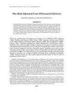
Figure 1 depicts the performance of bank stocks relative to the broad markets index for the
countries included in our sample. There is a common pattern across all markets. Bank stocks
performed strongly between 1999 and 2008, but they hugely underperformed during the
last five years. Indeed, banks in the EMU countries performed the worst since 2007. In less
than two years, the bank indices of both US and its EMU equivalent lost roughly 50 % of
their market value. Both indices reached their lowest level in March 2009. Thanks to
extensive government and central bank help, confidence and liquidity then slowly returned
to the markets.


72

Maher Asal

As seen from the figure, equity price declines have been the most obvious for European
banks, which are more exposed to European government securities, and could be affected
by growth crunches in the Euro area. Indeed, banks in European countries have performed
the worst since 2007.

Figure 1: Banking Equity Performance Relative to Broad Index
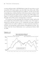
Figure 2 depicts the share of banking market capitalization relative to the overall market
capitalization. In all countries, this share grew substantially over the past two decades in
line with the increase in market activities. The market capitalization of European as well as
American banks saw a solid rise until late 2007. For example, at the end of 2007 banks
made up around 20 %, 17% and 9% of the overall market capitalization in the EMU, the
UK and the US, respectively. This was roughly double their share at the beginning of the
1990s, although only half that in 2009. Up to that point, developments in the overall market
value of the Eurozone and the US were closely correlated, entering into a sideward
movement. However, from 2011 on, they started to diverge strongly with shares
experiencing only a temporary setback in the US, but a fall without recovery in Europe due
to the European sovereign debt crisis. The market capitalization shares in the EMU, US,
UK and Sweden are currently 12%, 5%, 12% and 23%, respectively.


Estimating the Cost of Equity Capital of the Banking Sector in the Eurozone

73

Figure 2: Market Capitalization Ratio
Figure 3 depicts the price-to-book ratio as an indication of how much equity investors are
willing to pay for each net assets. Focusing on the comparison between the Eurozone and
US since 2010, visual inspection of the figure shows that the stock market is still clearly
skeptical about the future prospects of these banks, as shown in the valuation of price to
book. There are three possible explanations for this skepticism. First, the market may

perceive the book values for many banks as excessive due to nonperforming loans which
can end in bank failures and lead to existing banks’ recapitalization of bailouts, redemptions
on publicly funded deposit insurance, or both (Reinhart and Rogoff, 2009). Banks tend to
register nonperforming loans as fully performing even if the probability of repayments is
very low because writing down such loans would reduce the banks’ book value of equity
and Capital to Risk Weighted Assets Ratio (CRAR). The second possible reason for the
low price to book ratio is investors’ uncertainty of future returns on banks’ equity. If a
bank’s return is equal the cost of equity, then price to book value would be around one.
Thus, banks with low (high) profitability are expected to have low (high) price-to-book
value. Since an increase of sovereign default risk is priced by the market, banks with
substantial exposures to European government bonds have experienced big drops in their
market value. Even banks without direct exposures to European government securities have
also been affected, as they have claims on banks highly exposed to sovereign debt. In
addition, the restructuring of Greek sovereign debt, which resulted in a 70 percent NPV
value loss for bondholders, has caused doubt on the efficiency of hedging instruments such
as credit default swaps (CDS) and drove sovereign bond prices downwards ( Jorge et al ,
2012)


74

Maher Asal

Figure 3: Price–to-Book Ratio
While the banking sector index, market capitalization and price-to-book ratio depict the
general trend in bank equity prices, it is silent about the drivers of their cost of equity capital.

3 Literature Review of Bank Cost of Equity
The cost of equity capital is an expected rate of return that cannot be directly observed from
the market, and different measures have been used in the literature. The first strand of

literature used the realized return, i.e. return on Equity (ROE) or Price/Earnings ratios, as a
proxy of the expected return or cost of equity. Zimmer and McCauley (1991) estimated the
real cost of equity for 34 international banks from six countries over the period 1984–90.
They used the cost of equity as a proxy by using the return on equity (ROE). They found
that Japanese banks enjoy a low cost of capital, German and Swiss banks face a moderate
cost of capital, and the US, UK and Canadian banks confront a high cost of capital. They
traced the differences to shareholders’ valuations of banks’ earnings in different equity
markets, difference in national saving behavioral and macroeconomic stabilization process.
Maccario et al (2002) investigated the cost of tier 1 capital of major banks from twelve
countries from 1993 until 2001. They estimated the cost of equity for the banking sector,
defined as the inverse of price earning (PE) in G-10 countries using earning’ forecasts rather
than historical earnings. They found that the estimated average costs of equity of major
banks in G-10 countries have been decreasing during the nine-year period from 1993 to
2001, and that the estimated costs of equity of individual banks are strongly related to both
microeconomic and macroeconomic variables. The problem with this approach is that a
historical return ignores risk. Consequently, its adaption as a performance measure may
result in a distortion of shareholder value. Competition among banks could lead to a ROE
race in which high targets are set. Attaining such a target given the current very low-risk
free rate would be difficult without experiencing considerable business and financial risk


Estimating the Cost of Equity Capital of the Banking Sector in the Eurozone

75

and increased fear for regulators. The recent financial crisis reveals the need to incorporate
risk considerations into the cost of equity.2
To incorporate risk into the cost of equity other studies used the Capital Asset Price
(CAPM) to estimate the cost of equity. Green et al (2003) analyzed the methods used by
the Federal Reserve to estimate the cost of equity for US banks. They found that the method

used in estimating the average bank’s cost of equity until 2002 was a combination of the
historical average of earnings, the discounted value of expected future cash flows, and the
equilibrium price of investment risk as per the capital asset pricing model. They showed
that the current approach would have provided stable and sensible estimates of the cost of
equity capital for the private sector adjustment factor (PSAF). Barnes and Lopez (2006)
tested whether the CAPM estimates were robust to changes in the size of the peer group,
the introduction of additional factors and variations in the calculation method. They
concluded that the cost of equity estimates based on averaging CAPM estimates across a
group of banks were reasonable for the purposes of the Federal Reserve System, which
therefore adopted the method as the sole approach for estimating the bank cost of equity as
of 2006. King (2009) estimated the real cost of equity for banks headquartered in six
countries over the period 1990–2009. The estimates were based on the single-factor CAPM
model used by the Federal Reserve System. The real cost of equity decreased steadily across
all countries except Japan from 1990 to 2005, but then it rose from 2006 onwards. A recent
report released by the Association for Financial Professionals (AFP), 2013, which allows
companies to compare techniques against those of other organizations, reveals that the
Capital Asset Pricing Model (CAPM) remains the one most commonly used by
practitioners and financial advisers to estimate a firm’s cost of equity. Although the CAPM
is useful in estimating what the hypothetical cost of equity of a bank is supposed to be in a
market’s equilibrium and remains the most commonly used by practitioners and financial
advisers to estimate a firm’s cost of equity, it is imprecise to estimate the true cost of equity
for a bank, given the possibility of market imperfections. In addition, problems arise when
banks from different countries are compared as the systematic risk factors that affect stocks’
returns can be significantly different among countries.
To overcome the problems arising from CAPM, other recent studies use the multi-factor
model. Although this approach seems appealing because it counts for other risk factors
besides market risk, challenges remain to identify these factors affecting the cost of equity
in the banking sector. Schuermann and Stiroh (2006), for example, used the three-factor
model to evaluate the impact of increased noninterest income on equity market measures
of return and risk of U.S. bank holding companies from 1997 to 2004. They used the

standard Fama-French factors and additional factors thought to be particularly relevant for
banks such as interest and credit variables. In addition to the market beta, they have
included the yield on a 3-month treasury bill, the spread between 10-year and 3-month
treasury rates, the spread between the Moody’s Baa-rated corporate bonds and 10-year
Treasury rates. He found that the three-factor model accounted for the largest proportion of
the systematic risk in individual bank stocks. Stiroh (2006) investigated whether additional
factors, such as different interest rate spreads, can explain bank-level equity returns, but he
did not find strong evidence supporting that fact. They concluded that the market factor
2

Rizzi (2014) argues that the appropriate measure of performance is the spread between ROE and
the cost of equity. Banks with ROE greater than the cost of equity are creating shareholder value and
trade at a multiple of book value. He shows that the spread between ROE and cost of equity times
the bank's book value is a bank’s economic profit.


76

Maher Asal

clearly dominates in explaining bank returns, followed by the Fama-French factors. Jorge
et.al (2012) studied the drivers of equity returns in the banking sector of advanced
economies. The drivers analyzed were sovereign risk, economic growth prospects, funding
conditions, and investor sentiment or risk aversion, Euribor-OIS spread, Sovereign CDS
spread, and some bank-specific factors. They found that a higher capitalization and lower
leverage made banks’ equity returns more resilient to adverse economic and sovereign risk
shocks. They also found that tier 1 capital to risk-weighted assets had an insignificant effect.
Demirgüç and Huizinga (2010) found that equity returns in the banking sector in the wake
of the Great Recession and the European sovereign debt crisis have been mainly driven by
weak growth prospects and heightened sovereign risk and to a lesser extent, by deteriorating

funding conditions and investor sentiment. They argued that a stronger capital position is
associated with better stock market performance, most markedly for larger banks, and that
the relationship is stronger when capital is measured by the leverage ratio rather than the
risk-adjusted capital ratio. These results are consistent with our results.
Yang and Tsatsaronis (2012) analyzed the impact of leverage, business cycle and the value
of book to market n banks’ stock return in the Euro area, US, UK, and Japan for the period
1989-2011. They found that the financing of the returns of bank equity is cheaper in the
boom and more costly during a recession. They provide support for prudential tools that
give incentives for banks to build capital buffers at times when the cost of equity is lower.
In addition, banks with higher leverage face a higher cost of equity, which suggests that
higher capital ratios are associated with lower funding costs.
The new regulatory framework of higher capital requirements was pointed out as an
important determinant of the cost of equity capital in the banking sector and gave rise to
several studies to quantify the impacting consequences. The empirical evidence for the
impact of regulation on a bank’s cost of equity is still ambiguous. Two opposite views
merged. The first view is based on the theorem of Modigliani-Miller (MM), 1958, which
argues that an increase in the cost of capital caused by a higher proportion of equity will,
under some assumptions, be offset by a reduction in the cost of equity. Subsequently, this
effect offsets the additional cost of a higher proportion of expensive equity capital in the
balance- sheet so that the overall cost of capital is unchanged. Many recent studies support
the (MM) theorem. Kashyap and Stein (2010) analyzed the impact of an increase in the
level of core equity on banking activities assuming that the increase of the cost of capital
will be completely echoed on the cost of credit. They make their study on a sample of large
U.S. banks over the period 1976-2008 in order to quantify the impact. They found that to
the extent that they are properly phased in, substantially higher capital requirements for
significant financial institutions are likely to have only a modest impact on the cost of loans
for households and corporations. This impact is, in and of itself, probably not sufficient to
be a major cause for concern. A similar study led by the European Central Bank (ECB
(2011) supports the MM theorem and the beneficial effect of an increase in the riskweighted capital ratio for a sample of 54 banks over the period 1995-2011. Similarly, Miles
et al. (2012) estimated the costs and benefits of new capital requirements on a panel of six

banks in the United Kingdom over the period 1997-2010. They proposed to analyze the
impact of a leverage reduction on the risk level and ultimately on the weighted average cost
of capital. BIS (2012) provides a strong argument for a banking recapitalization in good
times. They also demonstrated that higher capital ratios are associated with lower funding
costs. More stringent capital standards can reduce not only the level of debt and the funding
cost but also that part of the volatility that is not aligned with the stock market. Schich and
Lindh (2012) found that implicit guarantees imply a very significant funding cost


Estimating the Cost of Equity Capital of the Banking Sector in the Eurozone

77

advantages for the banks that benefit from them. They thus create distortions to competition
and an invitation to use them and, perhaps, take on too much risk
The second is the view of the banking and financial industry, which holds that an increase
in the proportion of equity, the most expensive form of capital, will negatively affect bank’s
profitability and increase funding costs which, in turn, leads to a credit crunch and a
decrease in economic growth (IIF, 2011). Their argument is that the initial hypothesis made
by MM (no taxes, no frictions and no information asymmetries) does not completely fit
reality because of the nature of banking activity and the size of the off-balance sheet
activities in this sector. They argue that a higher ROE will be commanding on the short
term in order to encourage investors to subscribe to the stock capital of new banks. Such a
reaction is in competition with less regulated non- bank issuers offering higher yields. In
addition, the risk-taking problem represents another distortion to the MM theorem. The
explicit guarantees (insurance of deposits) present serious alterations with lower financing
rates for banks than for firms in other sectors. As for implicit guarantees (government
insurance) it implies a part of the default risk of the bank moves to tax-payers, which allows
debt issuers to receive a premium on debt.
Finally, a large body of literature analyzes the impact of macroeconomic factors on stock

market returns (Prabha and Wihlborg, 2014, and Zhi et al, 2012). A business cycle, for
example, can influence bank equity prices through its impact on bank assets. During a
boom, the default rate of loans to households and firms decline. This, in turn, boosts bank
earnings and can mitigate investors´ perceptions of the risk. Barth et al (2013) provided a
new data and measures of bank regulatory and supervisory policies in 180 countries from
1999 to 2011. Their measures were based upon responses to hundreds of questions,
including information on permissible bank activities, capital requirements, the powers of
official supervisory agencies, information disclosure requirements, external governance
mechanisms, deposit insurance, barriers to entry, and loan provisioning. They analyzed
changes in bank regulatory and supervisory practices over time, examined the degree to
which banking policies had converged across countries, and documented how the
organization of bank regulatory authorities and the size and structure of the banking system
differed around the world. They found that, although there was some convergence along
some dimensions of bank regulation, substantial heterogeneity remained in policies,
organization, and structure.

4 A Conceptual Framework for Measuring the Cost of Equity
4.1 Model Specification
Measurement of the cost of equity is probably the most challenging and controversial topic
in corporate finance literature. This is because the cost of equity capital is an expected rate
of return, thus it cannot be directly observed from the market.


78

Maher Asal

The recent literature reviewed above revealed that two foremost approaches can be used for
estimating the cost of equity: the capital asset pricing model and the multi-factor model3.
4.1.1 Capital Asset Pricing Model (CAPM), the One –Factor Beta model

The CAPM, developed by Sharpe (1964), Lintner (1965a,b) and Mossin (1966) is a widely
used model to estimate the cost of equity for individual companies. It a is a general
equilibrium model that quantifies the relationship between risk and expected return using a
single risk factor and remains the most widely used approach in practice for estimating the
cost of equity for individual companies as well as a measure of performance for portfolio
managers (Campbell et al., 1997, and King, 2009). CAPM postulates that the nominal cost
of equity capital (or expected return) for a bank is linearly determined by the nominal riskfree rate and a firm-specific risk premium and assumed to follow a simple one-factor model:
𝐸(𝑅𝑖 ) = 𝑅𝑓 + 𝛽𝑖𝑚 (𝐸[𝑅𝑚 ] − 𝑅𝑓 ) + 𝜀𝑖,𝑡

(1)

Where 𝐸(𝑅𝑖 )is the expected return (cost of equity) for bank i, 𝐸[𝑅𝑚 ]is the expected return
on the overall market portfolio, 𝑅𝑓 is nominal yield on the risk-free asset, 𝛽𝑖𝑚 is the equity
beta (load factor) that measures the sensitivity of a bank’s equity return to the market, and
𝜀𝑖,𝑡 is a purely idiosyncratic shock assumed to be uncorrelated across banks. The term
(𝐸[𝑅𝑚 ] − 𝑅𝑓 ) is the equity market risk premium which measures the average annual return
that investors may be expected to earn on their equity portfolio relative to the risk-free rate.
Equation (1) states that the only source of systematic risk is the market factor. The
assumption in equation (1) is that historical returns are a good proxy for expected returns
are approximately independently and identically distributed (IID) through time and jointly
multivariate normal.
4.1.2 Multi-Beta Models
In spite of its popularity in academics and the real financial world, empirical support for
the CAPM is poor, casting doubt about its ability to clarify the actual movements of asset
returns. Its inadequacies have also threatens the way it is used in applications. The main
empirical shortcoming of the CAPM is that a single market factor is not sufficient to explain
the cross-section of realized returns, as understood in the large amount of studies of CAPM
anomalies.
Empirical evidence suggests that additional factors may be required to adequately
characterize behavior of expected stock returns and logically leads to the consideration of

multi-beta pricing models. A more complicated asset pricing model consists of multi-beta
framework is required in the form of the Arbitrage Pricing Theory (APT), developed by
Ross (1976). The APT - is based on arbitrage arguments and assumes:
𝐸(𝑅)𝑖 = 𝑅𝑓 + 𝛽1 𝑋 1 + ⋯ 𝛽𝑘 𝑋𝑘 + 𝜀𝑖,𝑡
3

(2)

The discounted dividends model can also be used to estimate the cost of equity. However, there are
a number of practical problems associated with this approach as highlighted by Ross et al. (2006)).
First, the model is applicable only to companies that pay dividend. Second, the estimated cost of
equity is very sensitive to the estimated growth rate. Third, the approach does not consider risk
factors.


Estimating the Cost of Equity Capital of the Banking Sector in the Eurozone

79

Where 𝐸(𝑅)𝑖 the cost of equity capital, and βk is measures the sensitivity of a bank’s return
to the kth economic factor. Given the economic factors, the parameters in the multi-beta
model can be estimated from the combination of time-series and cross sectional regression
(i.e. panel data), see
Jagannathan and Wang (1998). However, the major problem with the multi-beta models is
that that economic theory does not specify the factors to be used in the models, so that there
is no consensus on the factors. The task of identifying the factors is left to empirical
research. Three main approaches have been used in the empirical literature to identify the
factors affecting the cost of equity capital. The first approach relies on using economic
intuition. Chen et al (1986), for example, selected five economic factors: the market return,
industrial production growth, the default premium, the term premium, and inflation. The

second approach is based on statistical analysis to extract factors from a cross section of
stock returns (Connor and Korajczyk, 1986). The last, and the one used in this paper, is to
identify factors based on empirical observation. An example of this approach is the threerisk-factor pricing model developed by Fama and French, 1993, reviewed below.
The three-risk-factor pricing model combines the Capital Asset Pricing Model (CAPM)
with two additional pricing factors identified by Fama and French (1993) to explain the
cross-sectional and time variation of equity returns in excess of the risk-free rate.
Specifically, the typical specification of the model is of the form:
𝐸(𝑅)𝑖 = 𝑅𝑓 + 𝛽𝑖𝑚 (𝐸[𝑅𝑚 ] − 𝑅𝑓 )+𝛽𝐻𝑀𝐿 𝐻𝑀𝐿𝑡 + 𝛽𝑆𝑀𝐵 𝑆𝑀𝐵𝑡 + 𝜀𝑖,𝑡

(3)

Where HML and SMB are the differences between the returns on diversified portfolios of
high minus low book to market stocks and small minus big stocks, respectively. These three
factors are designed to capture the value and firm size effects that have long been
documented in empirical finance literature. If these factors are relevant for banks, they
should obviously have some statistical significance and increased explanatory power
relative to the CAPM in Eq. (1). Moreover, if these factors control for common variation
in bank returns, the cross-sectional residuals in Equation (3) should be less correlated than
in Equation (1).
Yang and Tsatsaronis (2012) augmented equation (3) by including three bank-specific
characteristics as additional drivers of the systematic risk in banks’ cost of equity: leverage,
earnings, and book-to-market valuation. Maccario et al (2002) emphasized the role played
by tier 1 capital ratio, the expected growth in earning, the payout ratio, and the gross rate
of loan losses as main the determinants of bank’s cost of equity. Jorge et al. (2012) showed
that the drivers of equity returns in the banking sector of advanced economies is affected
by sovereign CDS spread, economic growth prospects, funding conditions (approximated
by Euribor OIS spread), leverage, loan-to-deposit and tier 1 capital.
We augment equation (3) by including additional drivers for the systematic risk in banks’
cost of equity capital. In particular, we consider bank-specific characteristics: (i.e.,
leverage, tier1 capital, and loan to deposit), regulation (as in Barth 2013), business cycle,

and proxy for sovereign risk, and proxies for funding conditions as the main determinants
of cost of equity.
Our broadest model, therefore, combines the Fama-French three-factor model factors with
6 additional risks. The following multi-factor equation is estimated:


80

Maher Asal

𝐸(𝑅)𝑖 = 𝑅𝑓 + 𝛽𝑖𝑚 ( 𝐸[𝑅𝑚 − 𝑅𝑓 ]+𝛽𝐻𝑀𝐿 𝐻𝑀𝐿𝑡 + 𝛽𝑆𝑀𝐵 𝑆𝑀𝐵𝑡 + 𝐿𝐸𝑉𝐸𝑅𝐴𝐺𝐸 +
𝐿

TIER1 + 𝐷 + TERM + 𝑂𝐼𝑆 + 𝐶𝐷𝑆 + 𝐼𝑁𝐹 + +𝐷𝑈𝑀𝑅𝐸𝐺 + 𝐷𝑈𝑀𝐴𝐶𝑇 + 𝜀𝑖,𝑡

(4)

We refer to Equation (3) as the “Bank-Factor” model. Where 𝐸(𝑅)𝑖 is the expected rate of
return (cost of equity) given by the average return for each individual bank I, LEVERAGE
is the bank’s leverage, which is defined as the total asset to equity, TIER1 is tier 1 capital,
and L/D is the loan to deposit ratio which indicates how much a bank relies on wholesale
funding. The inclusion of the latter variable was justified, as the 2008 crisis showed that
banks were vulnerable to a run on wholesale funding (Duffie, 2010; Gorton and Metrick,
2010).
We also incorporated additional interest rate factors, as control variables, thought to be
particularly relevant to banks; the one-period change in the slope of the term structure
(TERM), defined as the difference between the 10-year and 3-month treasury rate. To
analyze the impact of sovereign risk on equity returns, we approximate sovereign risk with
the arithmetic average of the 5-year credit default swap (CDS) spreads. We also include the
3-month Euribor-EONIA spread (Euribor OIS spread) to account for funding conditions

and investor sentiment. To count for the impact of macroeconomic fundamentals on banks’
cost of equity, we include business cycle, approximated by the inflation rate.4 The high
minus low (HML) and small minus big (SMB) factors control for value and size premium
as in Fama and French (1993).
As the estimated cost of equity will be sensitive to the appropriate measure of risk-free rate,
Rf, and for the robustness of the results, we use three proxies for the risk-free rate in the
Euro Area. The first is the 1-month euro overnight index average swap rate (EONIA).
EONIA swaps are the most liquid instrument in the euro money markets. Since they are
mark-to-market on a daily basis and do not involve exchange of principal, the rates are less
affected by counterparty risk (Jorge et al., 2012). This is not the case for Libor rates, as
rising default risk in the banking sector has increased unsecured borrowing costs in the
interbank market. The second proxy is the 3- month money interbank rate, EURIBOR. The
third proxy is the German bond yields, which may reflect market concerns of the need to
bail out European countries. The proxies for the risk-free rate in the other countries are 3
month treasury bills in the US and UK, 1 month repo rate in Sweden, and Central bank
lombard rate in Switzerland. In addition, the changing of regulation and minimum capital
requirements following the international financial crisis are considered important
detriments for a bank’s cost of capital and the rates available to borrowers. Standard theory
predicts that, in perfect and efficient capital markets, reducing banks’ leverage (i.e., an
increase in equity capital) reduces the risk and cost of equity but leaves the overall weighted
average cost of capital unaffected (MM theorem).
Barth et al (2013) analyzed changes in bank regulatory and supervisory practices over time
and examined the degree to which banking policies have converged across 180 countries.
They constructed two indexes. The first is to measure the degree to which national
regulations restrict banks from engaging in (1) securities activities, (2) insurance activities,
and (3) real estate activities. The index values for securities, insurance, and real estate range
4

For the EMU we calculated the average of the 5-year credit default swap spreads for Belgium,
Germany, Estonia, Ireland, Greece, Spain, France, Italy, Cyprus, Latvia, the Netherlands, Austria,

Portugal, Slovenia, Slovakia and Finland. Two EMU countries are excluded due to the data being
unavailable.


Estimating the Cost of Equity Capital of the Banking Sector in the Eurozone

81

from 1 to 4, where larger values indicate more restrictions on banks performing each
activity. In particular, 4 signifies that an activity is prohibited, 3 indicates that there are tight
restrictions on the provision of the activity, 2 means that the activity is permitted but with
some limits, and 1 signals that the activity is permitted. They found a great cross-country
variability in the degree to which countries restrict banks from engaging in different
activities. The regulatory notion of a bank, therefore, differs markedly across countries —
and, this definition changes over time within the same country. Only Switzerland was to
grant banks unrestricted securities, insurance, and real estate powers. Most countries
tightened the overall restrictions on bank activities following the global financial crisis and
the introduction of Basel III. The second index is to measure the stringency of bank capital
regulations that measure the amount of capital banks must hold and the stringency of
regulations on the nature and source of regulatory capital. Larger values of this index of
bank capital regulation indicate more stringent capital regulation. Their results show that
most countries increased the stringency of their capital regulations following the crisis,
including the United States. In addition, Portugal, Belgium, Austria, Switzerland, Greece,
Cyprus, Finland, Ireland and the United Kingdom had reduced the stringency of their
capital regulations in the aftermath of the crisis.
We utilize the database of Barth et al. (2013) to track changes in regulation and supervision
since 1999 for the countries included in our sample by examining the change in the capital
regulatory restrictions index since 2007. Since the scope of permissible activities differs
across countries, banks are not the same across countries. In the empirical equation (4) we
use two different deregulatory dummies. The first is DUMACT, which takes the value of

unity if the country grant banks unrestricted securities, insurance, and real estate powers
(i.e., Switzerland) and zero otherwise. The second is DUMREG, which takes a value of
unity for banks with increasing stringency of their capital regulations following the crisis
(i.e. the US and EU). The εit is assumed to be independently distributed across individuals
with zero mean, but arbitrary forms of heteroskedasticity across units and time are possible.

4.2 Estimation Procedures
4.2.1 Data
This study uses a data sample of the largest 140 banks in developed economies (comprising
78 banks from the EMU, 33 banks from the US, 6 banks from the UK, 4 banks from
Sweden, and 19 banks from Switzerland). For a complete list of banks, see the Appendix.
The sample does not include delisted banks during the period 1999-2014, which may result
in survivorship bias. The results, therefore, could be biased towards banks with large
capital, banks thought too-big-to-fail that benefitted from an implied government
guarantee, and regional banks that were less affected by the ongoing financial crisis due to
their narrow international exposures. It is important to emphasize that, our aim is not to
develop a precise asset-pricing model per se Rather we take existing models, as defined by
risk factors, to explain common variation of banks’ costs of equity capital using panel data
regression. Monthly data series for bank-specific characteristics and country-specific
factors for the period January 1999 – March 2014 were collected from Datastream and
MSCI.


82

Maher Asal

4.2.2 Methodology
We use the dynamic panel system of the Generalized Method of Moments (GMM)
estimator as proposed by Arellano and Bover (1995) and Blundell and Bond (1998) that

allows economic models to be specified while avoiding needless assumptions, such as
specifying a particular distribution for the errors. As pointed out by Hall (2005), this lack
of structure in the GMM made it widely applicable in econometrics because competing
economic theories often imply that economic variables satisfy different sets of population
moment conditions. Furthermore, GMM controls for dynamic endogeneity arising from
ignored heterogeneity and simultaneity that might exist in the regression and it is robust to
model misspecification (Christensen et al, 2008). We use lagged values of the cost of equity
as instruments to controls for potential simultaneity and reverse causality. Thus, our
estimation procedure allows all the explanatory variables (i.e., bank-specific-factors and all
control variables) to be treated as endogenous.
4.2.3 Panel Unit-Root Tests
In order to investigate the possibility of panel cointegration, it is first necessary to determine
the existence of unit roots in the panel data series of Equation (4). A number of researchers,
especially Levin et al. (2002), Breitung (2005), Hadri (1999), and Im, Pesaran and Shin
(2003) have developed panel-based unit root tests that are similar to tests carried out on a
single series. Remarkably, these researchers have shown that panel unit root tests are more
powerful (less likely to commit a Type II error) than unit root tests applied individually. In
addition, in contrast to individual unit root tests, which have complex limiting distributions,
panel unit root tests lead to statistics with a normal distribution in the limit [see Baltagi,
2001]. Theoretically, these tests are essentially multiple-series unit root tests that have been
applied to panel data structures.
The Im, Pesaran and Shin (IPS, hereafter) test has been found to have superior test power
by researchers in economics to analyze long-run relationships in panel data, and we employ
this procedure in this study. IPS offers a test for the presence of unit roots in panels that
combines information from the time series component with that from the cross section
component, so that fewer time observations are required for the test to have power.
Following Startz (2013), an IPS test starts by specifying a separate ADF regression for each
cross-section with individual effects and no time trend:
pi

Δy it = α i + ρ i y i,t 1 + ∑ β ijΔy i,t j + ε it

(5)

j=1

where i = 1, . . .,N and t = 1, . . .,T
IPS use separate unit root tests for the N cross-section units. After estimating the separate
ADF regressions, the average of the t-statistics for p1 from the individual ADF regressions,

t iTi ( p i ) :

t NT =

1 N
∑ t (p β )
N i =1 iT i i

(6)

The t-bar is then standardized and it is shown that the standardized t-bar statistic converges
to the standard normal distribution as N and T   . IPS (1997) showed that a- t bar test
performs better when N and T are small.


Estimating the Cost of Equity Capital of the Banking Sector in the Eurozone

83

4.2.4 Panel Cointegration Tests

The next step is to test for the existence of a long-run cointegration among the cost of equity
and the independent variables in Equation (4) using panel cointegration tests. We use two
cointegration tests: the Kao (Engle-Granger based) and the Combined Fisher and Johansen
tests to determine the unrestricted Cointegration Rank to trace the maximum eigenvalue.
This panel cointegration test revealed to have more power than conventional cointegrated
test (Coiteux and Oliver, 2000).
The Kao (1999) test specifies cross-section specific intercepts and homogeneous
coefficients on the first-stage regressors. Generally, the Kao test considers running the first
stage regression in the form:
𝑦𝑖𝑡 = 𝛼𝑖 + 𝜕𝑖 𝑡 + 𝛽1𝑖 𝑥1𝑖,𝑡 + 𝛽2𝑖 𝑥2𝑖,𝑡 + ⋯ … 𝛽𝑀𝑖 𝑥𝑀𝑖,𝑡 + 𝑒𝑖𝑡

(7)

For t =1,…..,T; i= 1, ….,N; m=1,….,M; where y and x are assumed to be integrated of order
one, e.g. I(1). The parameters αi and ∂i are individual and trend effects which may be set to
zero if desired. A Kao test requires the αi to be heterogeneous, the βi to be homogeneous
across cross-sections, and all of the trend coefficients must be et to zero. Kao then runs
either the pooled auxiliary regression,
𝑒𝑖𝑡 = 𝜌𝜀𝑖𝑡−1 + 𝑣𝑖𝑡

(8)

Or the augmented version of the pooled specification:
𝑝

𝑒𝑖𝑡 = 𝜌̃𝑒𝑖𝑡−1 + ∑𝑗=1 𝜑𝑗 ∆𝑒𝑖𝑡−𝑗 + 𝑣𝑖𝑡

(9)

The Fisher (1932) test derives a combined test that uses the results of the individual

independent tests. Maddala and Wu (1999) use Fisher’s result to propose an alternative
approach to testing for cointegration in panel data by combining tests from individual crosssections to obtain a test statistic for the full panel. If πi is the p-value from an individual
cointegration test for cross-section , then under the null hypothesis for the panel,
2
−2 ∑𝑁
𝑖=1 log(𝜋𝑖 ) → 𝜒 2𝑁

(10)

By default, EViews reports the value based on MacKinnon et al (1999) p-values for
Johansen’s cointegration trace test and maximum eigenvalue test

5 Empirical Framework
Table 2 presents descriptive statistics of the cost of equity of banking sector as well as the
explanatory variables for the whole sample period. We highlight three points. First, on
average, the cost of equity capital in thee baking sector is about 8% which is lower than the
stock market returns of 8.13%. Second, the most volatile variables are CDS, HML and
SMB. Third, because many statistical inferences require that a distribution be
symmetrically and normal or nearly normal we report the values of skewness and kurtosis.
For all variables, except HML and SMB, the distribution is approximately symmetrical.
However, all variables exhibit excess kurtosis <0 (platykurtic). Exceptions are SMB, HML


84

Maher Asal

and CDS, which exhibit excess >0 (leptokurtic) and inflation with excess kurtosis = 0. The
table also reports a more solid test; the Jarque–Bera test to investigate the hypothesis that
the data are from a normal distribution. The null hypothesis is a joint hypothesis of the

skewness being zero and the excess kurtosis being zero. Since the Jarque-Bera test statistic
exceeds the critical values (reported below the table) for any reasonable significance level
for all variables, except inflation and TERM, we may conclude that the variables do not
follow a normal distribution.
Table 1: Descriptive statistics of the cost of equity capital and its determinants for 140
banks in the EMU, US, UK, Sweden and Switzerland.
Mean

Median

Max.

Min.

Std.

Skewness Kurtosis Jarque-Bera

Prob.

Obs.

RI

8,063

8,015

10,843 5,852

1,36

0,31

RF

0,03

0,029

0,064

RM

8,318

8,26

10,617 6,167

SMB

0,504

0,675

HML

0,111

LEVERGE 2,486

2,177

40,463

0

913

0,016 -0,234

1,977

48,149

0

913

1,115 0,168

2,403

17,868

0

913

22,321 -21,96 4,621 -0,454

5,899

305,615

0

795

0,155

26,347 -100

6,131 -4,704

81,593

237560,9

0

910

2,975

3,643

0,976 -1,184

2,785

210,568

0

894

0,002

0,483

TIER1

16,701 16,441

18,842 15,242 0,965 0,481

2,15

61,558

0

897

SPREAD

1,702

1,601

5,814

-1,708 1,459 0,152

2,654

4,167

0,12

471

TERM

0,516

0,51

3,63

-2,89

2,908

8,305

0,02

913

OIS

1,614

0,528

5,938

-0,103 1,754 0,837

2,268

62,774

0

451

CDS

158

48,36

1365

5,485

301,2 2,901

10,085

1268,431

0

363

L/D

1,313

1,242

2,617

0,294

0,401 0,387

2,691

25,956

0

897

INF

1,718

1,7

5,6

-2,1

1,241 0,052

3,029

0,439

0

911

1,4

-0,229

Where RI refers to the log of the average expected return for the banking sector. RF is the
risk-free rate, RM is the log of equity market rate of return, HML (high minus low) and
SMB (small minus big) are the differences between the returns on diversified portfolios of
high minus low book to market stocks and small minus big stocks, respectively.
LEVERAGE is the log of assets divided by Equity, TIER1 is the log of tier1 capital, L/D
is the log of loan deposit, SPREAD is the difference between the 10-year and 3-month

Treasury rates, CDS is the average of the 5-year credit default swap spreads, OIS is the 3month Euribor-EONIA spread, and INF is the inflation rate. The critical values of The
Jarque-Bera test for the chi-square distribution are: 4.61 5.99, 9.21 for significance level of
10%, 5% and 1%, respectively.
Table 2 reports the results of the IPS panel unit root test at level. The results shown in
column 2, with only constant, clearly show that the null hypothesis of a panel unit root
cannot be rejected for most of the variables (RI, RF, RM, LEVERAGE, L/D, TERM and
OIS). However, the null hypothesis of a panel unit root is rejected for HML, SMB, TIER1,
CDS, and INF. The results shown in column 3-with both constant and time trend, show
similar results except that the null hypothesis of a panel unit root cannot be rejected for
TIER 1 Capital. Table 2 also presents the results of the tests at first difference with only a
constant and constant plus time trend, column 5 and 6, respectively. The results evidently


Estimating the Cost of Equity Capital of the Banking Sector in the Eurozone

85

reject the null hypothesis of a panel unit root for all series in the first difference. We can
conclude that the series RI, RF, RM, LEVERAGE, L/D, TERM, TIER1 and OIS are nonstationary in level but stationary in the first difference, e.g. I(1). The series HML, SMB,
CDS, and INF are stationary in level, e.g. I (0). Given these results, it is possible to apply
panel cointegration tests in order to test for the existence of the stable long-run relation
among the variables.
Table 2: Panel Unit Root Test- Im, Pesaran and Shin W-statsticPS), for the period
1999(1)-2014(3), No of observation 908.
Variable
Constant
RI
RF
RM
HML

SMB
TIER1
LEVARGE
TERM
CDS
INF
l/d

0.582
(0.720)
0.132
(0.552)
1.570
(0.941)
-10.161*
(0.000)
-9.189*
(0.000)
3.893 *
(1.000)
-1.392
(0.081)
-0.956
(0.169)
-3.498 *
(0.002)
-4.159*
(0.000)
0.818
0.79

Level
Constant + Trend
1.195
(0.884)
-1.154
(0.124)
0.259
(0.602)
-9.616*
(0.000)
-8.448*
(0.000)
1.375
(0.915)
-1.412
(0.078)
-1.788
(0.036)
-3.199*
(0.000)
-3.851 *
(0.000)
0.858
(0.80)

Constant
-9.377
(0.000)
-8.197

(0.000)
-8.730
(0.000)

First Difference
Constant +
Trend
-8.667
(0.000)
-7.340
(0.000)
-8.158
(0.000)

-11.176
(0.000)
-11.82
(0.000)
-10.62
(0.000)

-11.226
(0.000)
-11.36
(0.000)
-9.93
(0.000)

-10.244
(0000)

-9.455
(0000)

Indicates rejection of the null hypothesis of no-cointegration at 1% levels of significance.
The critical values for rejection (probability) are: -2.99, -2.75 and -2.62, for 1%, 5%, and
10%, respectively. Numbers in parenthesis refer to the probability of significance.
Automatic selection of maximum lags and automatic lag length selection based on SIC. Eview 8 software of unbalanced panels of 183 observations been used.
The next step is to test for cointegration where the null hypothesis is no-cointegration. This
is to investigate whether long-run steady state or cointgration exist among the cost of equity
capital, RI, and the independent variables. We employ two cointegration tests: the Kao test
and the Combined Fisher and Johansen. Table 3 reports the results of both tests. In column
2, we found that the estimated ADF t-statistics of -2.858 to be statistically significant at 1
percent level, which rejects the null hypothesis of no cointegration. The results for the
Johansen Fisher Panel Cointegration Test, shown in column 4-8, confirm the presence of at
most 3 cointegration ranks independent with or without the inclusion of constant and trend.


86

Maher Asal

These results show existence of the stable long-run relation among the variables in equation
(3).
Table 3: Results from cointegration test of factors determining the cost of equity capital
for banking sector. Sample: 1999M01 2014M03. Null Hypothesis: No cointegration.
Johansen Fisher Panel Cointegration Test. Unrestricted
Kao Residual
Cointegration Rank Test (Trace and Maximum
Cointegration Test

Eigenvalue)
tStatistics Prob.*
Fisher
Fisher Stat.
ADF -3.258
0.001
Stat. From
From maxADF -3.638
.001(a) No. of CE(s)
Trace test Prob.* eigen test
1- No Trend in Data
(a) No intercept or trend in CE or VAR
None
55,260
0,000 45,870
At most 1
377,700
0,000 42,740
At most 2
84,690
0,000 35,800
At most 3
52,380
0,000 23,180
At most 4
31,350
0,000 12,580
(b) Intercept in CE and no trend in VAR
None
682,700

0,000 96,180
At most 1
129,700
0,000 53,140
At most 2
82,580
0,000 30,250
At most 3
45,850
0,000 18,550
At most 4
28,660
0,000 8,543
2-Linear Trend in Data
(a) Intercept in CE or VAR
None
286,000
0,000 80,360
At most 1
125,100
0,000 52,930
At most 2
71,420
0,000 31,180
At most 3
43,680
0,000 18,380
At most 4
26,030
0,000 9,272

(b) Intercept and trend in CE and no trend in VAR
None
379,600
0,000 92,440
At most 1
561,000
0,000 109,300
At most 2
59,030
0,000 25,590
At most 3
53,370
0,000 21,110
At most 4
32,180
0,000 10,430

Prob.*

0,000
0,000
0,000
0,001
0,050
0,000
0,000
0,000
0,000
0,000

0,000
0,000
0,000
0,005
0,159
0,000
0,000
0,000
0,002
0,108

Newey-West automatic bandwidth selection and Bartlett kernel. Included observations:
915. Series: ln(RI), RF, ln(RM), ln(TIER1), ln(LEV), ln(L_D), TERM, HML, SMB,
CDS, INF, DUMREG, and DUMACT.

5.1 Results
Various dynamic specifications of the panel GMM were estimated using Equation (4) to
control for the endogeneity bias (reverse causality) running from the cost of equity capital
to the explanatory variables. In addition, we used the lag of the explanatory variables and
various instrumental variables to circumvent the endogeneity problem posed. Table 4
reports the results of the GMM estimation of the cost of equity of the banking sector with


Estimating the Cost of Equity Capital of the Banking Sector in the Eurozone

87

fixed effect using several regressions, all stemming from our initial specification. The
second column (specification 1) reports the results of CAPM estimates that take into
account the stringency of regulations and permissible activities captured by DUMREG and

DUNACT, respectively. The third column (specification 2) shows the results of the threefactor model. The purpose here is to test if the additional two variables, HML and SMB add
any explanatory power to the cost of equity banking. Column 4 and 5 (specifications 3 &
4) show the results of two stipulations of Equation 4. The aim here is to test if the bankspecific factors, country-specific factors, and the change in regulations and the funding
structure of banks, as imposed by the new so-called Basel III standards, affect a bank’s cost
of equity capital. The regressions seem satisfactory in terms of goodness of fit and statistical
significance. Based upon these regressions we obtain predicted banks’ costs of equity for
the years 1999(1)-2014(3) that are not significantly different from the corresponding actual
values5. On the basics of these results, it is possible to maintain that the model shows a good
degree of reliability in estimation the cost of equity.
We now turn our attention to the economics of the Bank-Factor Model (Equation 4). The
question of interest is which particular factors are considered the most important
determinants of the cost of equity in the banking sector? Focusing on statistically and
economically significant variables of specification 4, the main results are as follows. First,
the value of the loading factor (beta) is around 1 and has the correct sign as expected by the
theory and highly significant at 1% significance level. Second, the dummies for banks
granted unrestricted activities (DUMACT) and stringency of bank capital regulations
(DUMREG) proved to be significant at different significance levels. That is, while
strengthened regulation led to an increase in the cost of equity for the banking sector,
relaxing the overall restrictions on bank activities increased the cost of equity capital in this
highly regulated-sector. Third, HML (value premium) and SMB (size premium) seem to be
insignificant explanatory variables that can determine the cost of equity for the banking
sector independent of the specification used. Fourth, an increase in the term structure (i.e.,
a positive yield curve), with other factors being equal, has a negative impact on a bank’s
cost of equity. The value of the coefficient is - 0.213, which is significant at 1 % level. This
result supports the findings by Schuermann & Stiroh (2006). Although the risk free variable
is significant in all specifications the sign is negative, contrary to what theory would predict.
This is probably due to a collinearity or over-specification problems.
Fourth, in contrast to previous studies, e.g. Maccario et al. (2002)), a higher tier 1 capital
ratio is associated with a higher cost of equity. Thus, adequate capital buffers as indicated
by Basel III reduce a bank’s probability of default but increase the cost of equity. The value

of the coefficient is 0.258, which is significant at 1% significance level. These results
support the findings of IIF (2011) and suggest that equity is more expensive than debt and
any increase in the proportion of equity, the most expensive form of capital, will increase
the cost of equity capital and probably increase the funding costs. Fifth, the cost of equity
capital seems to be explained by the leverage. An increase in equity ratio so a decrease in
leverage will increase the cost of equity capital (expected return). The value of the
coefficient is 0.803, which is significant at 1% significance level. Thus the MM principle
is not revealed. A higher proportion of equity and therefore a reduction in leverage lead to
an increase in the expected yield by investors (cost of equity). This may explain why banks
generally feel compelled to operate in such a highly-leveraged fashion, in spite of the
obvious risks this poses. After all, debt is cheaper than equity, helps to maximize ROE, and
5

These estimates have not been reported but available upon request.


88

Maher Asal

provides a tax shield. In addition, debt has government guarantees (explicit and implicit).
This fact is the most important reason why banks prefer leverage. Non-banks do not lever
as much as banks because they do not have these guarantees. The result regarding long-run
effects of the leverage on the cost of equity opposes the findings of Yang & Tsatsaronis
(2012) who found that a decline in leverage (i.e. an increase in equity financing) lead to a
decline of the cost of equity capital. Our findings, however, support the results of Jorge et
al. (2012), who found that lower leverage was associated with higher equity performance.
Thus, a leverage reduction as stipulated in the Basel III framework will increase the cost of
equity. As leverage decreases, the advantageous of implicit guarantees funding also
decreases.

Sixth, as the loan-to-deposit increases the cost of equity decreases. The value of the
coefficient is -1.13, which significant at 1% significance level. A result that supporting
Jorge et al. (2012) who find a negative and significant impact of loan-to-deposit ratio on
the rate of return for European banks between 2009-2011. Seventh, the impact of CDS
turned out to be significant and negative determinants of the cost of equity capital. The
value of the coefficient is -0.001, which is significant at 1% significance level. Our findings
add a new breadth to the common belief that credit derivatives such as the credit default
swap (CDS) have lowered the cost of firms’ debt financing by creating for investors new
hedging opportunities and information. Ashcraft and Santos (2007), for example, argue that
because speculators can take short (long) positions in credit risk by buying (selling)
protection without needing to trade the cash instrument and because these potentials are
hard to replicate in the secondary loan or bond markets, the prices of CDS are considered a
special source of new information about firms. Duffie (2008), on the other hand, provides
alternative ways where banks can use credit derivatives to hedge their exposures to
borrowers. Finally, inflation turned out to be insignificant determinants of the cost of equity
capital.


Estimating the Cost of Equity Capital of the Banking Sector in the Eurozone

89

Table 4: 1-step GMM estimation of the cost of equity capital for banking with a fixed
effect.6
Variables
Constant
RM
DUMREG
DUMACT

Specification 1
-1,165*
-7,528
1,114*
61,825
0,200*
4,508
-0,536*
-9,932

Specification 2
-1,191*
-7,13
1,117*
57,304
0,334*
6,587
-0,536*
-9,804

LEVERAGE
LTIER 1
L/D
SMB

Specification 3
-3,597*
-8,524
1,365*
46,751

0,524*
9,512
-0,736*
-11,868
-0,399*
-11,673
0,076*
3,037
0,264*
3,19

-0,005
-1,232
0,001
-0,098

HML
TERM
INF
CDS
R-squared

0,812

0,811

0,846

Specification 4
-7,381*

-18,042
1,579*
39,054
0,270**
2,612
-0,09
-1,601
-0,803*
-22,386
0,258*
10,246
-1,139*
-8,423
0,003
0,682
0,001
-0,003
-0,213*
-14,682
-0,012
-0,833
0,001*
-5,641
0,958

In sum, the results of our Bank-Factor Model show that loading factor, regulations,
leverage, tier 1 capital and the loan-to-deposit ratio are the most important factors for
determining the cost of equity for the banking sector. While an increase in loading factor,
tier 1 capital and regulations, increase the cost of equity, an increase in leverage and loanto-deposit, decrease the cost of equity for the banking sector.

5.2 Do the Drivers of Cost of Equity Capital vary across Vountries?
To check robustness, we investigate the extent to which the drivers of the cost of equity
capital vary across the EMU, US and UK. We run three separate panel regressions using
data samples of the largest 78 banks from the EMU, 33 banks from the US, and 6 banks
from the UK. Focusing on the comparison between the EMU and the US, the results shown
6

We examined the presence of perfect multicollinearity using the t-test of correlation coefficients as
well as Variance Inflation Factors (VIF). The results, not shown but could be provided upon request,
show the absence of perfect multicollinearity in the regression.


90

Maher Asal

in Table (5) show that the drivers of the cost of equity in the EMU are different from the
US in three aspects. The first is related to the impact leverage. While leverage affects the
cost of equity negatively in the US, it asserts no impact in the EMU. For EMU banks, the
results suggest that the compensation effect of MM theory is revealed. An increase in equity
proportion, the most expensive sort of capital (i.e., a decrease in leverage) is offset by a
reduction in the expected rate of return as investors anticipate a lower risk to be incurred.
Yet, the impact is statistically insignificant with a coefficient value.
Table 5: GMM estimation of the cost of equity capital for the banking sector; cross
country
EMU
US
UK
RF
0,206**

2,331*
-0,460***
2,548
3,029
-2,231
RM
1,286*
1,081*
0,803**
8,264
14,710
2,613
LEVERAGE
0,162
-3,215*
0,635
1,331
-2,815
1,722
LTIER1
-0,279*
-0,172**
-0,048
-3,585
-2,542
-0,240
L/D
0,286
-0,529*
0,053

3,030*
-4,019
0,126
HML
-0,005**
0,011**
-0,002
-2,272
2,573
-0,335
SMB
0,006
-0,001
-0,001
0,996
-0,314
-0,123
TERM
0,024
0,023
0,300*
0,222
1,491
8,180
CDS
0,001**
-0,002*
-0,002
-2,261
-3,287

-1,140
INF
-0,153*
-0,044*
0,077*
-2,815
-4,766
3,341
R-squared
0,929
0,924
0,707
Instrument specification: R, LRM, HML, SMB, LLEV, LTIER 1, LL_D, TERM, CDS,
and INF
This is a result that support the findings of Kashyap and Stein, 2010, King, 2009, ECB,
2011, Miles et al., 2012, and BIS, 2012). As for the US, the results shown in Table (5)
support our previous findings in Table (4) and suggest that, in contrary to MM theory, an
increase in equity proportion is associated with an increase in the expected rate of return.
The second is related to the impact of the loan-to-deposit. While loan-to-deposit affects the
cost of equity positively in the EMU, it has a significant and negative impact in the US.
The third is related to the impact of HML. While the HML affects the cost of equity
negatively in the EMU, it has a positive and significant impact in the US.


Estimating the Cost of Equity Capital of the Banking Sector in the Eurozone

91

6 Conclusion
This paper attempts to estimate the cost of equity capital for the banking sector using data

from the Eurozone, the US, the UK and Sweden for the period 1999-2014. We employ the
dynamic panel GMM model with a fixed effect and a multi-factor asset pricing framework
to estimate the cost of equity capital. Our results show that loading factor, regulations,
Leverage, tier 1 capital and the loan-to-deposit ratio are the most important factors for
determining the cost of equity for the banking sector. While an increase in loading factor,
tier1 capita and regulations, increase the cost of equity, an increase in leverage and loan-todeposit decrease the cost of equity for the banking sector. In contrast to the MM theorem,
our findings support the results of IIF (2011) in that a higher leverage ratio, an increase in
capital requirement and regulation results in an increase of the cost of equity in the banking
sector. To check robustness, we investigate the extent to which the drivers of the cost of
equity capital vary across the EMU, the US and the UK. We find that the drivers of the cost
of equity in the EMU are different from the US in three aspects. The first is related to the
impact leverage. While leverage affects the cost of equity negatively is the US, it asserts no
impact in the EMU. The second is related to the impact of loan-to-deposit. While loan-todeposit affects the cost of equity positively in the EMU, it has a significant and negative
impact in the US. The third is related to the impact of HML. While the HML affects the
cost of equity negatively in the EMU, it has a positive and significant impact in the US. The
scope behind these differences a topic for future research.

References
[1]

A. Ashcraft, and J. Santos, "Has the Credit Default Swap Market Lowered the Cost
of Corporate Debt’?” Federal Reserve Bank of New York Staff Reports, 2007.
[2] A. Hall, "Generalized Method of Moments’, Oxford University Press, Oxford, UK.
[3] A. Kashyap and J. Stein, "An Analysis of the Impact of “Substantially Heightened”
Capital Requirements on Large Financial Institutions," University of Chicago and
Harvard Working paper, 2010.
[4] A. Levin C. Lin and J. Chu, "Unit root tests in panel data: Asymptotic and finitesample properties J," Journal of Econometrics 108, 2002.
[5] A. Maccario A. Sironi, and C. Zazzara, "Is banks’ cost of equity capital different
across countries?" Evidence from the G10 countries major banks. Libera Università
Internazionale degli Studi Sociali (LUISS) Guido Carli, working paper, 2002.

[6] Association for Financial Professionals (AFP), "Current Trends in Estimating and
Applying the Cost of Capital," 2013.
[7] A. Jorge X. Estelle and J. Schmittmann, "Equity Returns in the Banking Sector in the
Wake of the Great Recession and the European Sovereign Debt Crisis," IMF working
paper no WP/12/174, 2012.
[8] Rossi and A. Timmermann,”What is the shape of the risk-return relation’? Social
Science Research Network,"Atlanta Meetings Paper, 2010.
[9] B.H. Baltagi, "Econometric Analysis of Panel Data,"2nd edition, John Wiley & Sons,
LTD., 2001.
[10] Basel Committee on Banking Supervision," Basel III: A global regulatory framework
for more resilient banks and banking systems," Bank for International Settlements,
2011.


92

Maher Asal

[11] BIS,” Post-crisis evolution of the banking sector’, Annual Report, 2012, pp. 64-92.
[12] Christensen, R. Poulsen, and M. Sørensen,"Optimal inference in dynamic models
with conditional moment," D-CAF Working Paper No. 30, 2008. Series Centre for
Analytical Finance, University of Aarhus.
[13] C. Kao, "Spurious regression and residual‐based tests for cointegration in panel data,"
Journal of Econometrics 90, 1999, 1–44.
[14] C. M Reinhart & K.S Rogoff, " This Time Is Different: Eight Centuries of Financial
Folly," Princeton, NJ: Princeton University Press, 2009.
[15] D. Duffie,"Presidential Address: Asset Price Dynamics with Slow-Moving Capital,"
The Journal of Finance VOL 4, 1992.
[16] D. Duffie, "Innovations in credit risk transfer: implications for financial stability," BIS
Working Papers No 255, 2008.

[17] D. Miles J. Yang, and G. Marcheggiano, "Optimal bank capital. 2012," The Economic
Journal, 2012.
[18] D. Zhi R. Guo, and R. Jagannathan, "CAPM for estimating the cost of equity capital:
interpreting the empirical evidence," Journal of Financial Economics, Vol 103, 2012,
pp 204–20.
[19] E. Green, J. Lopez and Z. Wang, "Formulating the Imputed Cost of Equity Capital for
Priced Services at Federal Reserve Banks,"Economic Policy Review, Vol .9, No.3,
2003.
[20] European Banking Authority," Final report on the implementation of Capital Plans
following the EBA‟s 201,"Recommendation on the creation of temporary capital
buffers to restore market confidence, 2012.
[21] European Central Bank report 2011, "Financial stability Review.
[22] F. E. Fama and K.R. French, "Common Risk Factors in the Returns on Stocks and
Bonds,” Journal of Financial Economics. 33:1, 1993, pp. 3–56.
[23] F.E. Fama and K.R. French, "Multifactor Explanations of Asset Pricing Anomalies,"
Journal of Finance 51:1, 1996, 1996, 55-84.
[24] F.E. Fama and K.R. French, "The Capital Asset Pricing Model: Theory and
Evidence,"Journal of Economic Perspectives 18:3, 2004, 25-46.
[25] F. Modigliani and & M. Miller, " The cost of capital, corporation finance and the
theory of investment’, American Economic Review, 1958, pp. 261-97.
[26] G. Connor, and R. Korajczyk, "Performance measurement with the arbitrage pricing
theory: A new framework for analyses," Journal of Financial Economics 15, 1986,
373-394.
[27] G. Gorton and A. Mterick, "Regulating the Shadow Banking System,"Brookings
Papers on Economic Activity, 2010.
[28] G.S Maddala and S. Wu, "A Comparative Study of Unit Root Tests with Panel Data
and A New Simple Test," Oxford Bulletin of Economics and Statistics 61, 1999.
[29] I. Choi,"Unit root tests for panel data," Journal of International Money and Finance
20, 2001.
[30] Im, K, Pesarann, H & Shin, Y 2003, ‘Testing for unit roots in heterogeneous panels,"

Journal of Econometrics 115: 53–74, 2005.
[31] Independent Commission on Banking, "Final Report recommendations," September
201.
[32] Institute International Finance, "The cumulative impact on the global economy of
changes in the financial regulatory framework," Washington, 2011.


Estimating the Cost of Equity Capital of the Banking Sector in the Eurozone

93

[33] J. Breitung, and S. Das, "Panel unit root tests under cross-sectional dependence,"
Statistica Neerlandica 59, 2005, 414–433.
[34] J.B. DeLong, and K. Magin, "The US equity return premium: past, present and
future," Journal of Economic Perspectives, no 23, 2009, pp 193–208.
[35] J. Lintner, "The Valuation of Risk Assets and the Selection of Risky Investments in
Stock Portfolios and Capital Budgets," Review of Economics and Statistics’, 47,
February 1965a, pp. 13–37.
[36] J. Lintner, "Security Prices, Risk and Maximal Gains from Diversification,"Journal of
Finance, 20, December 1965b, pp. 587–615.
[37] J. G. MacKinnon A. Haug and L. Michelis, "Numerical Distribution Functions of
Likelihood Ratio Tests for Co‐integration ," Journal of Applied Econometrics 14,
1999, 563‐577.
[38] J. Mossin,”Equilibrium in a Capital Asset Market," Econometrica. October, 35, 1966,
pp. 768–83.
[39] J. V. Rizzi, "Calculate Cost of Equity to Truly Measure a Bank's
Performance,"American Banker November 21, 2014.
[40] J. Shambaugh, "The Euro’s Three Crises," Brookings Papers on Economic Activity,
2012.
[41] J. Yang and K. Tsatsaronis, "Bank stock returns, Leverage and the Business Cycle,"

BIS quarterly review, 2012.
[42] J.Y. Campbell, A.W. Lo, and A.C. MacKinlay,"The Econometrics of Financial
Markets," Princeton University Press, Princeton, 1997.
[43] K.A. Demirgüç, and H. Huizinga, " Are Banks Too Big to Fail or Too Big to Save?"
International Evidence from Equity Prices and CDS Spreads’, European Banking
Center Discussion Paper No 2010-15, 2010.
[44] K. Hadri, "Testing the Null Hypothesis of Stationarity Against the Alternative of a
Unit Root in Panel Data with Serially Correlated Errors," Manuscript Department of
Economics and Accounting, University of Liverpool, 1999.
[45] K. Stiroch, "A Portfolio View of Banking with Interest and Noninterest Activities,"
Journal of Money, Credit and Banking Vol. 38, 2006, No. 5.
[46] M. Arellano, "On the testing of correlated effects with panel data," Journal of
Econometrics, 59, 1995.
[47] M. Arellano, and O, Bover," Another look at the instrumental variables estimation of
error-components models," Journal of Econometrics, 68, 1995, 29–51.
[48] M. Coiteux, and S. Olivier,"The Saving Retention Coefficient in the Long Run and in
the Sort Run: Evidence from Panel Data," Journal of International Money and
Finance, 19, 2000, 535-548.
[49] M.L. Barnes, and J.A. Lopez,” Alternative measures of the Federal Reserve Banks
cost of equity capital," Journal of Banking and Finance, no 30, 2006, pp 1687–711.
[50] M. Prabha and C. Wihlborg, " Implicit Gurantees, Business Models and Banks Risktaking through the crisis: Global and European Perspective," Journal of Economics
and Business, 2014.
[51] N. Bryan, and R. Sengupta,"Global European Banks and the Financial Crisis’, Federal
Reserve Bank of St. Louis Review," November/December 94(6), 2012, pp. 457-79.
[52] N. Chen, R. Roll & S. Ross," Economics Forces and Stock Markets’. Journal of
Business, Vol.59, No.3, 1986, 383-403.
[53] N. Dews, N. Hawkins and T. Horton, "Measuring the cost of Capital in Australia,"
Research discussion paper no 9205, June 1992.