Using principal components analysis to model interest rate moves and measure delta exposure: A comprehensive breakdown of a Lebanese commercial bank’s portfolio
Bạn đang xem bản rút gọn của tài liệu. Xem và tải ngay bản đầy đủ của tài liệu tại đây (192.41 KB, 8 trang )
Journal of Applied Finance & Banking, vol. 5, no. 1, 2015, 143-150
ISSN: 1792-6580 (print version), 1792-6599 (online)
Scienpress Ltd, 2015
Using Principal Components Analysis to Model Interest
Rate Moves and Measure Delta Exposure: A
Comprehensive Breakdown of a Lebanese Commercial
Bank’s Portfolio
Viviane Y. Naimy 1
Abstract
This paper quantifies exposure to all the possible ways the Lebanese yield curve changed
since 2006. It studies the interest rate risk impact on a portfolio consisting of interest-rate
depending assets belonging to a Lebanese commercial bank using principal components
analysis or risk decomposition strategy. TBs monthly yields are used with five different
maturities since 2006. Deltas for the portfolio are calculated using partial duration and the
DV01. The first factor identified corresponds to a parallel shift in the yield curve and the
second to a change of slope of the yield curve. Both factors account for 95% of the
variance. Delta exposure calculations showed absence of hedging against these shifts.
JEL classification numbers: C10, C18
Keywords: Interest Rate Risk; Lebanese banks; Delta Exposure; Delta Hedging;
Principal Components Analysis; Risk Management; Partial Duration
1 Introduction
Risk management is now a must for all corporations and particularly for financial
institutions. They have no choice but to increase the resources they allocate to risk
management. “Subprime” losses at banks would have been avoided if risk management
techniques had been properly implemented to detect the unacceptable level of risks taken
and accurately take the right decisions to minimize the total risk they have faced.
Regulators have refined their requirements in order to avoid bankruptcy - that arises from
1
Dr., Professor of Finance, Faculty of Business Administration & Economics, Notre Dame
University- Louaize, Lebanon.
Article Info: Received : September 10, 2014. Revised : October 8, 2014.
Published online : January 1, 2015
144
Viviane Y. Naimy
incurred losses - and bankruptcy costs and recently most financial institutions are heavily
regulated. Throughout the world, and after the large bail-outs of financial institutions in
2008, governments seek financial stability. Financial stability involves confidence in
financial institutions. In other words, regulators want to ensure that capital held by a bank
is sufficient to provide a cushion to absorb the losses with a high probability (Basel
Committee on Banking Supervision, July 2009 [1], and December 2010 [2]). They are in
fact concerned with total risks. Two approaches to risk management are open to financial
institutions to manage market risk: risk decomposition and risk aggregation.
The purpose of this paper is to use the risk decomposition strategy in order to study the
interest rate risk impact on a portfolio consisting of interest-rate depending assets
belonging to a Lebanese commercial bank, classified as “Alpha 2 ” bank. Factors
affecting the interest rate moves are identified. Zero-coupon yield curve are used to
consider both parallel and nonparallel shifts. The paper implements the principal
components analysis to handle the risk arising from highly correlated variables. TBs
monthly yields 3 are used with five different maturities since 2006. Given that there is a
complete absence of academic work dealing with delta exposures of the Lebanese banks’
portfolios, this paper serves as a guide for the implementation of delta exposure using the
principal components analysis.
The paper proceeds as follow: Section 2 presents a panoramic review of managing market
risk techniques through delta, gamma and vega. It also covers the VaR technique together
with the three methods of estimating the VaR. The portfolio structure together with the
model implementation using the principal components analysis and delta exposure
calculation are evaluated and analyzed in section 3. Assessment of the importance of the
different yield curve shifts is also depicted in section 3. The paper then concludes the
empirical findings.
2 Review on Market Risk and Market Risk Management
Market risk is the uncertainty of cash flows and potential for loss associated with
movements in an underlying source of risk such as interest rates, foreign exchange rates,
stock prices, or commodity prices. When analyzing interest rate risk, there is the risk of
short-, intermediate-, and long-term interest rates. Within short-term interest rate risk,
there is the risk of LIBOR changing, the risk of the Treasury bill rate changing, the risk of
the commercial paper rate changing and many other risks associated with specific interest
rates [3]. The extent to which those rates are correlated must be considered by risk
managers. The effect of changes in the underlying source of risk will be reflected in
movements in the values of spot derivative positions. Delta, Gamma and Vega are all risk
measures equally applicable to many instruments in addition to options and stocks. They
are some of the tools used by risk managers to control market risk [4].
Delta hedging consists of making the portfolio be unaffected by small movements in
interest rates. Delta calculation is needed by taking the mathematical first derivatives of
2
An Alpha bank is classified among the top ten banks in Lebanon in terms of total assets and
liabilities.
3
It is quite impossible to obtain time series data due to the lack of transparency and data
availability.
A Comprehensive Breakdown of a Lebanese Commercial Bank’s Portfolio
145
the swap or option value with respect to interest rates. Therefore a delta-hedged position
is one in which the combined spot and derivatives positions have a delta of zero. The
portfolio would then have no gain or loss in value from a small change in the underlying
source of risk. Larger movements, however, can bring about additional risk not captured
by delta. This requires a Gamma 4 hedge by combining transactions so that the delta and
gamma are both zero. The portfolio would then have no gain or loss in value from a small
change in the underlying source of risk. Moreover, the delta itself would be hedged,
which provides protection against larger changes in the source of risk [5]. Unfortunately
the use of options introduces a risk associated with possible changes in volatility. This
risk is hedged by Vega 5. A portfolio of derivatives that is both Delta and Gamma hedged
can incur a gain or loss even when there is no change in the underlying as a result of a
change in the volatility.
In spite of a dealer’s efforts at achieving a delta-gamma-vega neutral position, it is
impossible to achieve an absolute perfect hedge. The vega hedge is accurate only for
extremely small changes in volatility. Large changes would require yet another
adjustment. In addition, all deltas, gammas, and vegas are only valid over the next instant
in time. Rarely will the end user engage in the type of dynamic hedging of
delta-gamma-vega neutral position. In fact the end is not typically a financial institution
like the dealer. Financial institutions can nearly always execute transactions at lower cost
and can afford the investment in expensive personnel, equipment, and software necessary
to do dynamic hedging. Most end users enter into derivatives that require little or no
adjustments. However, many suffered losses from being unhedged at the wrong time or
from outright speculating. Most end users could have obtained a better understanding
about the magnitude of their risk and the potential for large losses had they applied the
Value at Risk, VaR [6&7].
VaR is widely used by dealers, even though their hedging programs nearly always leave
them with the little exposure to the market. The basic idea behind VaR is to determine the
probability distribution of the underlying source of risk and to isolate the worst given
percentage of outcomes. Loosely, VaR summarizes the worst loss over a target horizon
that will not be exceeded with a given confidence level. Using 5% as the critical
percentage, VaR will determine the 5% of outcomes that are the worst. The performance
at the 5% mark is the VaR. There are three methods of estimating the VaR [8].
The analytical method, also called the variance-covariance method, makes use of
knowledge of the input values and any necessary pricing models along with an
assumption of a normal distribution. In other words, it uses knowledge of the parameters
of the probability distribution of the underlying sources of risk at the portfolio level. Since
the expected value and variance are the only two parameters used, the method implicitly
is based on the assumption of normal distribution. If the portfolio contains options, this
assumption is no longer valid because option returns are highly skewed and the expected
return and variance of an option position will not accurately produce the wished result. In
e − d1 /2
Using the Black-Scholes-Merton Model: Call Gamma =
S0 σ 2πT
2
4
2
5
S T e -d1 /2
Using the Black-Scholes-Merton Model: Call vega = 0
2π
146
Viviane Y. Naimy
this case, another alternative is used and employs the delta rather than the precise option
pricing model to determine the option outcome. This is called the delta normal method
and is only approximate. It linearizes the option distribution by converting the option’s
distribution to a normal distribution. This is useful when a large portfolio is concerned.
For long periods, the delta adjustment is sometimes supplemented with a gamma
adjustment [9].
Secondly, the historical method estimates the distribution of the portfolio’s performance
by collecting data on the past performance of the portfolio and using it to estimate the
future probability distribution. It assumes that the past distribution is a good estimate of
the future distribution. Obviously it matters greatly whether the probability distribution of
the past is repeated in the future. Also the portfolio held in the future might differ from
the one held in the past. Another problem is that the historical period may be badly
representative of the future.
Monte Carlo Simulation Method combines many of the best properties of the previous
two methods. It is the most widely used method by sophisticated firms. It generates
random outcomes based on an assumed probability distribution to obtain the VaR.
Portfolio returns can be easily simulated. This requires inputs on the expected returns,
standard deviations, and correlations for each financial instrument. It is a flexible method
since it allows the analyst to assume any known probability distribution and can handle
complex portfolios. It is also the most demanding method in terms of computer
requirements and the most efficient among risk management techniques.
In this paper, we will focus on following the risk decomposition strategy to measure the
interest rate risk of an interest-rate dependant asset portfolio of a Lebanese commercial
bank using principal component analysis.
3 Principal Components Analysis and Delta Exposure
3.1 Data, Sample Selection, and Partial Duration
The selected portfolio, belonging to a Lebanese commercial bank rated among the top
10% in terms of total assets among all the operating commercial banks in Lebanon,
consists of long positions in interest-rate dependent assets and is worth USD 10 million.
We considered the monthly changes of the Lebanese TBs with maturities of 3 months, 6
months, 1 year, 2 years and 3 years from January 2006 up to June 2014. Table 1 depicts
the summary statistics of these rates during the mentioned period.
A Comprehensive Breakdown of a Lebanese Commercial Bank’s Portfolio
147
Table 1: Summary Statistics for the Lebanese TBs for the Period Jan 2006 through June
2014
3 Months
6 Months
1 Year
2 Years
3 Years
Mean
4.6575
5.873
6.249
6.974
7.964
Variance
0.2530
1.352
1.546
1.944
2.163
Std. Dev.
0.5030
1.163
1.243
1.394
1.471
Skewness
-0.1670
0.1441
0.2099
0.2353
-0.1915
Median
4.4400
5.230
5.400
5.930
8.850
Mode
5.2200
7.240
7.750
8.680
9.540
Minimum
3.8900
4.430
4.790
5.410
5.970
Maximum
5.2200
7.240
7.750
8.680
9.560
Range
1.3300
2.810
2.960
3.270
3.590
1st Quartile
4.4300
4.990
5.350
5.930
6.610
3rd Quartile
5.2200
7.240
7.750
8.680
9.540
Table 2 depicts the partial duration of the portfolio. The partial duration calculation is
based on the selected zero-coupon yield curve for the chosen maturities based on the
median corresponding percentages and a 1% change for each point on the zero curve.
Rates on the shifted curve are calculated using linear interpolation.
Maturities
Duration (Di)
Where 𝐷𝐷𝑖𝑖 =
Table 2: Partial Duration for the Portfolio
3 Months
6 Months
1Year
2 Years
0.1
0.12
0.2
0.6
3 Years
1.2
Total
2.22
1 ∆𝑃𝑃𝑖𝑖
𝑃𝑃 ∆𝑦𝑦 𝑖𝑖
3.2 Deltas for the Portfolio using DV01
Analysts usually calculate several deltas to reflect their exposures to all the different ways
in which the yield curve can move. We will compute the impact of a one-basis-point
change for each point on the yield curve. A measure related to this delta is DV01. This
delta is the partial duration multiplied by the value of the portfolio multiplied by 0.0001
as shown in table 3.
Maturities
Delta
Table 3: Deltas for the Portfolio
3 Months
6 Months
1Year
100
120
200
2 Years
600
3 Years
1200
Unfortunately, the Lebanese banks do not use interest rate deltas to hedge their portfolios
despite the simple structure of those portfolios. Some banks divide the yield curve into a
number of segments to calculate the impact of changing the zero rates corresponding to
each segment by one basis point while keeping all other zero rates constant.
148
Viviane Y. Naimy
3.3 Deltas for the Portfolio using Principal Component Analysis
Principal Component Analysis is a standard tool with many applications in risk
management. It takes historical data on changes in the market variables and attempts to
define a set of factors that explain the movements. The aim is to replace the five variables
by a smaller number of uncorrelated variables. The market variables we will consider are
the TB rates with the above defined maturities. We first calculated a covariance matrix
from the data. This is an 5x 5 matrix where (i,j) entry is the covariance between variable i
and variable j. We then calculated the eigenvectors and eigenvalues for this matrix. The
eigenvectors are chosen to have length 1. The eigenvector corresponding to the highest
eigenvalue is the first principal component.
The interest rate move for a particular factor is the factor loading. Factor loadings have
the property that the sum of their squares for each factor is 1.0. The interest rate changes
observed on any month is expressed as a linear sum of the factors by solving a set of five
simultaneous equations. The first factor, PC1, in table 4 corresponds to a parallel shift in
the yield curve. One unit of that factor makes the 3-month rate increase by 0.352 basis
points, the 6-month rate increase by 0.542 basis points, the one, two and three-year rates
by 0.517, 0.529, and 0.181 basis points respectively. The second factor corresponds to a
change of slope of the yield curve. Rates between 3 months and 1 year move in one
direction, the remaining move in the other direction. The third factor is obviously not
significant. This is shown by the standard deviation of its factor score. The standard
deviations of the factor scores are shown in table 5 and the factors are listed in order of
their importance. It can be seen that the first factor accounts for 57.46% of the variance 6
in the original data and the first two factors account for 95% of the variance.
3 Months
6 Months
1 Year
2 Years
3 Years
Table 4: Eigenvector Factor Loadings 7 for TBs Data
PC1
PC2
PC3
PC4
0.352673
-0.07694
-0.69177
0.618004
0.542451
-0.0717
-0.37647
-0.7464
0.517475
-0.10497
0.513261
0.164123
0.529925
-0.10865
0.340836
0.181715
0.181022
0.982911
0.010877
0.03154
PC5
-0.09606
-0.0419
-0.65637
0.747118
0.001911
In other words, a quantity of the first factor equal to one standard deviation corresponds to
the 3-month rate moving by 5.66 8 basis points. Same analysis is applied to the remaining
variables. Table 6 illustrates those moves for the first two factors. It is worth mentioning
that the factor scores are uncorrelated across the data: the parallel shift is uncorrelated
with the change of the slope of the yield curve.
6
Which is 449.23
A factor is not changed if the signs of all its factor loadings are reversed.
8
0.352*16.066 = 5.65 bp.
7
A Comprehensive Breakdown of a Lebanese Commercial Bank’s Portfolio
PC1
Table 5: Standard Deviation of Factor Scores 9
PC2
PC3
PC4
PC5
16.066
12.986
3.2856
2.6711
Table 6: TBs rate Moves
PC1
In basis points
3 Months
6 Months
1 Year
2 Years
3 Years
149
2.1212
PC2
5.666044
8.715018
8.313753
8.513775
2.908299
-0.99914
-0.9311
-1.36314
-1.41093
12.76408
We conclude that most of the risk in interest rate moves is accounted for by the first two
factors (figure 1) and that we can solely relate the risks in this Lebanese portfolio to
movements in these factors instead of all five rates.
Figure 1: The most Two Important Factors Affecting TBs Rates
1
0.8
0.6
0.4
PC1
0.2
PC2
0
-0.2
3M
6M
1Yr
PC2
PC1
2Yrs
3Yrs
4 Discussion and Conclusion
The advantage of using principal components analysis is that it indicates the most
appropriate shifts to consider while providing information on the relative importance of
these shifts [10]. Also, it gives an alternative way of calculating deltas. After measuring a
one-basis-point change in the five different maturities of the portfolio, it becomes
9
The square root of the ith eigenvalue is the standard deviation of the ith factor score.
150
Viviane Y. Naimy
straightforward to use the first two significant factors to model rate moves and calculate
the delta exposure of the portfolio. Therefore, delta exposure to each of the selected
factors can be measured in dollars per unit of the factor with the factor loading being
assumed to be in basis points 10. Both deltas are positive and greater than one and
consequently the portfolio lacks all hedging plans and strategies. Despite the limitations
of this study regarding the absence of daily data and the absence of transparency as to the
hedging strategies, we were able to quantify in a detailed manner the exposure to all the
possible ways the Lebanese yield curve changed since 2006. This constitutes an absolute
added value to the very limited existing academic work covering risk management in
Lebanon.
There is a lot to be done for Lebanon in the area of risk management. So far what has
been discussed in this paper has been of an analytical and quantitative nature. However,
the Lebanese banks did not yet recognize that there is a great deal to know about risk
management that is not based on words and wishes. We are not sure if the Lebanese
banks’ infrastructure is conductive to the practice of risk management. All of the
quantitative models and analytical knowledge would be wasted if banks cannot
implement sound risk management. Risk management is effective only if people apply
these techniques in a truthful and responsible manner with the required controls. We are
not sure how far the Lebanese banks are accurately practicing risk management.
References
[1]
Basel Committee on Banking Supervision, Basel III: A Global Regulatory
Framework for More Resilient Banks and Banking Systems, (December 2010).
[2] Basel Committee on Banking Supervision, Guidelines for computing Capital for
Incremental Risk in the Trading Book, (July 2009).
[3] P. Jorian, The financial Risk Manager Handbook, New York, Wiley, (2001-2002).
[4] J. Hull, Risk Management and Financial Institutions, 3d ed. Wiley, (2012).
[5] D.M. Chance, An introduction to Derivatives & Risk Management, 6th ed.
Thomson-South-Western, (2004).
[6] V. Naimy, The German and French Stock Markets Volatility as Observed from the
VaR Lens, American Journal of Mathematics and Statistics, 4(1), (2014), 7-11.
[7] V. Naimy, Parameterization of GARCH(1,1) for Paris Stock Market, American
Journal of Mathematics and Statistics, 3(6), (2013), 357-361.
[8] P. Jorian, Value At Risk: a New Benchmark for Controlling Financial Risk, 3d ed.
McGraw-Hill, (2007).
[9] D.M. Chance, An introduction to Derivatives & Risk Management, 6th ed.
Thomson-South-Western, (2004).
[10] R. Reitano, Nonparallel Yield Curve Shifts and Immunization, Journal of Portfolio
Management, (1992), 36-43.
For instance, Delta Exposure to Factor 1 (PC1) = ∑5𝑖𝑖=1 ∆𝑖𝑖 𝑥𝑥𝑃𝑃𝑃𝑃1𝑖𝑖 where ∆𝑖𝑖 represents the
change in the portfolio value for a 1-bp move for each of the five maturities, and 𝑃𝑃𝑃𝑃1𝑖𝑖 are the factor
loading values per maturity and in bp.
10