Determinants of financial and temporal endurance of commercial banks during the late 2000s recession: A split-population duration analysis of bank failures

Journal of Applied Finance & Banking, vol. 6, no. 4, 2016, 1-16
ISSN: 1792-6580 (print version), 1792-6599 (online)
Scienpress Ltd, 2016

Determinants of Financial and Temporal Endurance of
Commercial Banks during the Late 2000s Recession: A
Split-Population Duration Analysis of Bank Failures
Xiaofei Li1 and Cesar L. Escalante2

Abstract
This paper presents an application of the split-population duration model in identifying
operating strategies and structural attributes of commercial banks that increased their
financial and temporal endurance (translated into probability and duration of survival,
respectively) during the late 2000s recession. This study’s results identify the isolated
effects of certain variables on a bank’s temporal endurance that have not been captured by
other commonly used survival models. For instance, delinquency rates for consumer and
industrial loans have separate adverse effects on the banks’ chances of survival and
temporal endurance, respectively, while real estate loan delinquency rates negatively affect
both survival parameters. Aside from the loan portfolio composition effects, interest rate
risk, fund sourcing strategies, and business size could also significantly influence a bank’s
survival through the financial crises.
JEL classification numbers: C41, G21, Q14
Keywords: Agricultural loans, real estate loans, bank failures, proportional hazard model,
late 2000s recession, loan diversification, split population duration model

1 Introduction
The National Bureau of Economic Research (NBER) contends that the late 2000s economic
recession caused some serious economic repercussions for the local and global economies
(NBER, 2010). This most recent recession, characterized by high unemployment, declining
real estate values, bankruptcies and foreclosures, affected the banking industry so severely
that nearly 500 banks failed from 2007 until the end of 2014. During this time, the number

1
2

Department of Agricultural and Applied Economics, University of Georgia, Athens, GA, USA.
Department of Agricultural and Applied Economics, University of Georgia, Athens, GA, USA.

Article Info: Received : April 19, 2016. Revised : May 12, 2016.
Published online : July 1, 2016


2

Xiaofei Li and Cesar L. Escalante

of critically insolvent banks included in the “High Risk of Failing Watch List” maintained
by Federal Deposit Insurance Corporation (FDIC) also increased dramatically.
Daniel Rozycki, associate economist of Federal Reserve Bank of Minneapolis, actually
pointed out some similarities of the late 2000s recession to the 1980s farm crisis in recent
agricultural sector trends (Rozycki, 2009). He observed that the prices of some key crops
doubled or tripled from 2006 to 2008 but started on a downhill trend thereafter (except in
2012 and 2013) while farmland prices were falling after reaching record high levels in 2008.
There has been some concern that a continued decline in land and crop prices could lead to
deterioration in the agricultural loan portfolios of commercial banks and other farm lenders.
It has been argued that no financial crisis can be dismissed as insignificant since any crisis
that affects all or even just a part of the banking sector may result in a decline in
shareholders’ equity value, the loss of depositors’ savings, and insufficient funding for
borrowers. These would translate to increasing costs on the economy as a whole or parts
within it (Hoggarth et al. 2002). In this regard, it is important to probe more deeply and
understand the causes of the bank failures experienced in the banking industry during the

last recession as this could provide insights on more effective, cautious operating decisions
that could help prevent the duplication of failures in the future.
Most early warning banking studies that have already been published have employed
probit/logit techniques in their analyses (Cole and Gunther, 1998, Hanweck, 1977, Martin,
1977, Pantalone and Platt, 1987, Thomson, 1991). The analyses are usually focused on
identifying retroactive determinants of a bank’s probability of failure versus survival.
Duration (hazard) models were introduced as an alternative to the probit/logit technique in
identifying the determinants of the probability of bank failure. The original application of
this model was introduced by Cox in a biomedical framework (Cox, 1972). In banking, the
Cox proportional hazard model was first applied in 1986 to explain bank failure (Lane et
al., 1986). The cox model adopts a semi-parametric function that offers the advantage of
avoiding some of the strong distributional assumptions associated with parametric survivaltime models. However, just as in other parametric duration models, the Cox proportional
model suffers from one shortcoming whereby it forces the strong assumption of the
eventual failure of every single observation analyzed by the model. Hence, the model is
incapable of isolating specific determinants of bank failure from factors that influence the
timing of failure.
The split-population duration model was conceived as a remedy to such shortcoming. The
model was first used by Schmidt and Witte (1989) in a study on making predictions on
criminal recidivism. The study recognizes the irrationality in assuming that every individual
would eventually return to prison. As such, the study’s sample has been “split” into those
that “(did go) back to prison” and “(did) not (go) back to prison”. The model was actually
applied to the analyses of bank failures in previous economic episodes other than the more
recent banking crises caused by the last recession (Cole and Gunter, 1995; Hunter et al.,
1996; Deyoung, 2003).
This paper presents an application of the split-population duration model to the banking
crisis in the late 2000s recession. Specifically, this article will identify early bank failure
warning signals that can be deduced from the operating decisions made and lessons learned
by banks that either failed or survived the last recession. This study differentiates itself from
previous empirical works through its focus on factors that affect both the comparative
financial (probability of survival) and temporal (length of survival) endurance of

commercial banks. The strength and reliability of this study’s results lie in its underlying
analytical framework’s capability to capture more realistic and intuitively reasonable


Determinants of Financial and Temporal Endurance of Commercial Banks

3

assumptions on the probability and timing of failure that should rectify results in other
studies that do not account for such conditions.

2 The Analytical Framework
This study’s analytical framework is derived from basic survival analysis techniques used
in previous empirical studies (Deyoung, 2003; Cole and Gunther, 1995; Schmidt and Witte,
1989). The likelihood function for the basic parametric survival model can be written as:
N

L   [f(t i | p,  )]1 Di [S(t i | p,  )]Di

(1)

i 1

where f (t) is the probability density function of duration t and S (t) is the survival
function. Di is the indicator variable that would equal to one if a bank survived the entire
sample period and would equal to zero if the bank was shut down during the period. As
pointed out in previous split-population duration studies (Schmidt and Witte, 1989, Cole
and Gunther, 1995, Deyoung, 2003), the basic duration model’s shortcoming lies in its
forced assumption that every observation in the dataset will eventually experience the event
of interest; or as applied to this analysis, the assumption that every bank would eventually

fail as time at risk becomes sufficiently large. The other shortcoming, as pointed out by
Cole and Gunther (1995), is that the likelihood function fails to distinguish between the
determinants of failure and those influencing the timing of failure. These issues are
addressed in the subsequent discussions.
Using the notation from Schmidt and Witte (1989), F is defined to be an unobservable
variable that equals to 1 if the bank eventually fails and 0 otherwise. Then,

P (F  1)   ,
P(F  0)  1  

(2)

where the estimable parameter  is the probability that a bank will eventually fail. With
this additional parameter, the basic likelihood function to be estimated is modified as
follows:
N

L   [ f(t i | p,  )]1 Di [(1   )   S(t i | p,  )]Di

(3)

i 1

If   1 , then the likelihood function reduces into a “basic” duration model that assumes
all banks will eventually fail. If   1, then both S (t) and f (t) are estimated conditional
on the probability of bank failure.
In bank failure studies, the log-logistic distribution has been widely used (Cole and
Gunther, 1995, Deyoung, 2003) since it is a non-monotonic hazard function that can
generate a hazard rate that increases initially before eventually decreasing. The log-logistic

4

Xiaofei Li and Cesar L. Escalante

distribution imposes the following form on the survival function S (t) and hazard function
h(t) :

S (t) 

1
1  ( t) p

(4)

h(t) 

f (t)  p( t) p 1

S (t) 1  ( t) p

(5)

Given the above, the shape of probability density function can be obtained from the product
of equations (4) and (5) as shown below:

 p( t)p 1
f (t)  S(t) h(t) 
[1  ( t) p ]2

(6)

where parameters p and  are positive parameters that define the exact shape of this
hazard function.
The probability of eventual bank failure  and the timing of failure  can be made bankspecific as follows:



1
1  e 'X
(7)

  e  ' X
where X is a vector of covariates that capture the influence of a bank’s financial condition
and the prevailing macroeconomic conditions on  and  .
The parameters  and  are estimated in the split-population duration model, with 
representing a direct relationship between bank specific covariates and the probability of
survival, and  indicating a direct relationship between those covariates and survival time.
The variables used in this study and their descriptive statistics are shown in Table 1. In
order to distinguish each variable’ effect on both the probability of survival and length of
survival, identical regressors are used in the estimation of α and β parameters. This
approach has been employed in several empirical studies (Douglas and Hariharan, 1994;
Cole and Gunther, 1995; DeYoung, 2003) and this study is an attempt to duplicate such
analytical method. The following sub-sections discuss the measurement of the explanatory
variables considered in this analysis and their expected relationships with the dependent
variables (also listed in Table 1).


Determinants of Financial and Temporal Endurance of Commercial Banks

5

Table 1: Definitions and summary statistics of duration model variables
Variables

Descriptions

Sample
Mean

Std.
Deviation

Min

Max

Expected Sign

Survival

Survival
Time

Dependent variable
T

Length of time between t=1
and the subsequent failure date
T

20.4287

2.5599

1

21

AGLOANS

Agricultural loans / total loans

0.0772

0.1275

0

0.7636

+/-

+/-

CONSUMLOANS

Consumer loans/total loans

0.0775

0.0880

0

1.0000

+/-

+/-

CILOANS

Commercial & Industrial loans
/ total loans

0.1530

0.0988

0

0.9668

+/-

+/-

REALESTNP

Aggregate past due/nonaccrual real estate loans/total
loans

0.0142

0.0198

0

0.3597

-

-

AGNP

Aggregate past due/nonaccrual agricultural loans/total
loans

0.0007

0.0039

0

0.1597

-

-

CINP

Aggregate past due/nonaccrual Commercial &
Industrial loans /total loans

0.0008

0.0023

0

0.0549

-

-

CONSUMNP

Aggregate past due/nonaccrual Consumer loans /total
loans
Herfindahl index constructed
from the following loan
classifications: real estate
loans, loans to depository
institutions, loans to
individuals, commercial &
industrial loans, and

agricultural loans.
Return on assets (Earnings)

0.0005

0.0023

0

0.0731

-

-

0.5606

0.1692

0

1.0000

-

-

0.0507

0.0481

-0.4452

0.4612

+

+

PURFUNDS

Purchased funds to total
liabilities

0.5085

0.1398

0

0.9952

-

-

DEPLIAB

Total deposits/ total liabilities

0.9254

0.0866

0.00001

0.9996

+

+

GAP

Duration GAP measure a

-0.0403

0.2100

-2.1587

0.9468

-

-

OVERHEAD

Overhead costs/total assets

0.0211

0.0115

0

0.3747

-

-

INSIDER

Loans to insiders/total assets

0.0154

0.0181

0

0.1973

-

+/-

SIZE

Natural logarithm of total
assets

11.8331

1.1820

8.1137

18.1842

+

+

Explanatory variables

HHI

PROFIT

a

GAP = Rate sensitive assets – Rate sensitive liabilities + Small longer-term deposits.


6

Xiaofei Li and Cesar L. Escalante

2.1 Asset Quality and Management Risk Variables
Bank loan concentration is measured in this model by HHI, calculated as the HerfindahlHirschman Index, which is bounded as follows:

1
 HHI  1
n
where n stands for the loan segments. This index will approach 1 under higher levels of
client specialization (or if banks tend to concentrate their loan portfolios around one or just
a few client categories). An index that approaches 0 indicates a more diversified loan
portfolio. This variable is designed to measure portfolio diversification that is usually
regarded as a risk reduction strategy (Markowitz, 1952; Thomson 1991; DeYoung and
Hasan, 1998). This index is expected to be negatively related to both the probability of
bank’s survival and expected survival time. 3
Management risk will be captured in the model by two measures: overhead cost ratios
(OVERHEAD) and insider loan ratios (INSIDER) (Whalen,1991; Thomson, 1991).
OVERHEAD is calculated as the sum of salaries and employee benefits, expense on
premises and fixed assets, and total noninterest expense divided by average total assets.
This ratio is expected to negatively influence the likelihood of survival since improved
management of these expenses would increase bank’s efficiency and therefore increase its
survival probability. The insider loan ratios (INSIDER) is calculated by dividing the
aggregate amount of credit extended to the banks’ officers, directors and stockholders to
total assets. Thomson (1991) used this ratio to capture management risk in the form of fraud
or insider abuse, and it is expected to be negatively related to both the probability of survival
and expected survival time.

2.2 Profitability Potential and Structural Variables
PROFIT, represented by the rate of return on assets, captures the banks’ earnings capability
and it is expected to increase both the probability of survival and expected survival time.

To capture the effect of the size and scale of banking operations, the logarithm of total
assets (SIZE) is included in this model (Cole and Gunther, 1995; Wheelock and Wilson,
2000; Shaffer, 2012). Compared to smaller banks that possibly do not have adequate
resource capability to withstand economic crises, larger banks are more likely expected to
survive since they possess greater financial flexibility and larger resource bases to weather
economic fluctuations.

3

The index was developed using Herfindahl measurement method where the index was constructed
from taking the sum of squares of various components of the loan portfolio:
𝑅𝑒𝑎𝑙 𝐸𝑠𝑡𝑎𝑡𝑒 𝐿𝑜𝑎𝑛𝑠 2
𝐿𝑜𝑎𝑛𝑠 𝑡𝑜 𝑑𝑒𝑝𝑜𝑠𝑖𝑡𝑜𝑟𝑦 𝑖𝑛𝑠𝑡𝑖𝑡𝑢𝑡𝑖𝑜𝑛𝑠 2
𝐻𝐻𝐼 = ∑{(
) +(
)
𝑇𝑜𝑡𝑎𝑙 𝐿𝑜𝑎𝑛𝑠
𝑇𝑜𝑡𝑎𝑙 𝐿𝑜𝑎𝑛𝑠
2
𝐼𝑛𝑑𝑖𝑣𝑖𝑑𝑢𝑎𝑙 𝐿𝑜𝑎𝑛𝑠
𝐶𝑜𝑚𝑚𝑒𝑟𝑐𝑖𝑎𝑙 𝑎𝑛𝑑 𝐼𝑛𝑑𝑢𝑠𝑡𝑟𝑖𝑎𝑙 𝐿𝑜𝑎𝑛𝑠 2
+(
) +(
)
𝑇𝑜𝑡𝑎𝑙 𝐿𝑜𝑎𝑛𝑠
𝑇𝑜𝑡𝑎𝑙 𝐿𝑜𝑎𝑛𝑠
2
𝐴𝑔𝑟𝑖𝑐𝑢𝑙𝑡𝑢𝑟𝑎𝑙 𝐿𝑜𝑎𝑛𝑠
+(
) }

𝑇𝑜𝑡𝑎𝑙 𝐿𝑜𝑎𝑛𝑠


Determinants of Financial and Temporal Endurance of Commercial Banks

7

2.3 Loan Portfolio Composition and Non-Performing Loan Variables
The banks’ loan exposures to different industry sectors are also accounted for in the model,
as suggested by previous literatures (Cole and Gunter, 1995; Wheelock and Wilson, 2000;
DeYoung, 2003). These variables include the proportion to total loans of loan exposures to
specific industry segments such as agriculture (AGLOANS), consumer
(CONSUMLOANS), and commercial & industrial (CILOANS) sectors.4 These variables’
impact on survival probability and time may vary depending on the relative financial health
of each sector.
The banks’ credit risk conditions are captured by several variables that capture the actual
delinquency rates experienced in certain loan categories. These categories or transaction
categories include agricultural (AGNP), real estate (REALESTNP), commercial and
industrial (CINP), and consumer (CONSUMNP) loan transactions. The aggregate value of
actual non-performing loans in each transaction category is calculated as the sum of “past
due up to 89 days”, “past due 90 plus days”, and “nonaccrual or charge-offs”. The measures
for these variables are calculated as the proportion of delinquencies in each transaction
category to the aggregate value of the loan portfolio in each category, and weighted by their
corresponding loan categories to total loan ratio.

2.4 Funding Arrangement Variables (FA)
Banks may hold portfolios of assets and liabilities with different maturities and a change in
interest rates will affect the portfolios’ market value and net income. Interest rate risk is
represented by three variables. The first variable is measured as the proportion of Purchased
Liabilities to Total Liabilities (PURFUNDS). As a price-taker in the national market, banks

that rely more on external markets through higher purchases of liabilities will incur greater
interest expenses and, hence, may have lower probabilities of survival (Belongia and
Gilbert, 1990).
The other measure is GAP (Belongia and Gilbert, 1990) and is derived by first subtracting
“liabilities with maturities less than one year” from “assets with maturities less than one
year” and then dividing the difference by total assets. This GAP ratio is expected to be
negatively related to both the probability of survival and survival time since banks can lose
their market value when interest rates rise.
The third variable, DEPLIAB, is calculated by taking the ratio of total deposits to total
liabilities. This ratio is expected to be positively related to the likelihood of survival and
bank’s survival time because bank’s tendency to thrive in the business is enhanced by their
ability to attract deposits to provide loans.

3 Data Description
The banking data used in this study are collected from the quarterly Consolidated Reports
of Condition and Income (call reports) published online by the Federal Reserve Bank of
Chicago (FRB). A dataset of banks that either failed or survived after December 2007
through the fourth quarter of 2012 was developed for this study. This time period
adequately captures the late 2000s recession, which was said to have formally started in
4

Real Estate Loans to Total Loan ratio is removed due to multicollinearity issue in this sample.


8

Xiaofei Li and Cesar L. Escalante

December 2007 (NBER, 2008). The reckoning (starting) point for each bank’s survival
period is set at the end of the 4th quarter of 2007. Some previous studies have considered

using time-varying covariates in their duration models applied to panel datasets (Wheelock
and Wilson, 2000; Dixon et al, 2011). However, Chung (1991) contends that the unique
design of the split-population duration model does not allow the explanatory variables to
vary over time while it is relatively straightforward and feasible to incorporate the timevarying design in a proportional hazard model. Hence, this analysis employs the more
applicable cross-sectional data analysis for its split-population model.
The maximum survival time is censored at 21 quarters. Banks that commenced operations
after December 2007 were not included in the dataset to ensure the right censoring of data.
The censoring design used in this analysis follows the approach used in earlier studies that
does not account for the censoring of failed banks (Cole and Gunter 1995; Deyoung 2003;
Maggiolini and Mistrulli 2005).5 Surviving or successful banks during the time period that
have missing values for any financial data being collected were discarded. Given these data
restrictions, the resulting sample of 6,839 banks consists of 6,461 surviving and 378 failed
bank observations. These banks’ financial performance indicators measured by the end of
2007 were used for this analysis.

4 Estimation Results
Prior to estimation, an important preliminary step is to check the appropriateness of the
distributional assumption by comparing the split-population’s hazard rate6 and the actual
hazard rate (Cole and Gunter, 1995; Douglas and Hariharan, 1994). This is achieved by
estimating a split-population model without covariates and comparing the predicted hazard
to a nonparametric estimate. The nonparametric hazard estimate is calculated by dividing
the number of failed banks at time t by the number of banks that neither failed nor were
censored in prior periods.

5

An interval censoring design approach is beyond the scope and capability of this paper, as has also
been the case of similar studies this article is drawn from. Future research efforts may be devoted
to validating the use of such design.
6

The hazard rate is calculated from an unconditional hazard function h(t)   (t) / [(1   )   S (t)] .


Determinants of Financial and Temporal Endurance of Commercial Banks

9

Hazard Rate
(Percent)
0.6

0.5

0.4
Split-population (loglogistic)

0.3

Nonparametric

0.2

0.1

0
2 3 4 5 6 7 8 9 10 11 12 13 14 15 16 17 18 19 20 21

Duration (Number of Quarters)
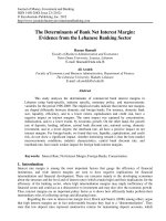
Figure 1: Estimated hazard rate for bank failure, 2008 Q1-2012 Q4
As shown in Figure 1, the nonparametric hazard rate rises rapidly from quarter 2 to quarter

8 (2009 third quarter) and would decrease at a slower pace from quarter 11 to quarter 21 (
S (T)  1 at quarter 1). This trend in the changes in the hazard rate is closely replicated by
the behavior of the forecasts by the split-population model using the log-logistic
distribution as the underlying parametric distribution.
Table 2 presents the estimation results for both the determinants of the probability of
survival and each bank’s survival time under the split population duration model.


10

Xiaofei Li and Cesar L. Escalante
Table 2: Maximum likelihood parameter estimates a and standard errors b for splitpopulation duration model

Variable

Split-Population Model †

Label



P-value

Survival
Intercept

<.0001

time
2.6189

(0.8027)
-0.0251
(0.1374)

P-value
0.0006

AGLOANS

Consumer loans

CONSUMLOANS

0.9304
(0.3255)

0.0021

0.3473
(0.2494)

0.0819

C&I loans

CILOANS

-0.2342
(1.9150)

0.4513

0.9773
(0.9876)

0.1612

Real Estate Nonperforming loan

REALESTNP

-19.4559
(3.3798)

<.0001

-3.8449
(0.5384)

<.0001

Ag Nonperforming loan

AGNP

-0.2247
(0.4967)

0.3255

-0.3573
(0.3048)

0.1205

C&I Nonperforming loan

CINP

-0.1779
(0.3792)

0.3195

-0.4654
(0.1395)

0.0004

Consumer Nonperforming loan

CONSUMNP

-0.9756
(0.6967)

0.0807

-3.4148
(4.5155)

0.2248

Herfindahl Index

HHI

0.0275

PROFIT

Purchased
Liabilities to total
liabilities
Deposits to
liabilities
Duration GAP

PURFUNDS

0.7827
(0.6772)
0.3780
(0.1326)
-0.2812
(0.1926)

0.1239

Profit

-2.2766
(1.1865)
0.9073
(0.2257)
0.9182
(0.5646)

0.0766

Overhead cost

OVERHEAD

Insider loan

INSIDER

Size, log(total
assets)

SIZE

0.5275
(0.3693)
0.0018
(0.0160)
0.1548
(0.1531)
0.3133

(0.1793)
-0.1072
(0.0330)

DEPLIAB
GAP

1.6242
(0.8828)
-0.4236
(0.0377)
0.3514
(0.7111)
-0.1262
(0.3572)
-0.4611
(0.0710)
3.8894
(0.2468)

0.1457

Survival

Ag loans

P
†

7.4449

(1.5131)
0.1752
(0.1661)



<.0001
0.0520

0.0329
<.0001
0.3106
0.3620
<.0001

0.4277

0.0022
0.0721

0.4541
0.1560
0.0403
0.0006

<.0001

Log likelihood at convergence is: -2032.6016, convergence criterion achieved is: 0.0100
Results in boldface are significant at least at the 90% confidence level.
b

Number in parentheses is the estimate’s standard error.
a


Determinants of Financial and Temporal Endurance of Commercial Banks

11

4.1 Determinants of the Probability of Survival
As laid out in this study’s analytical model, the covariates associated with  measure their
impact on the probability of a bank’s survival. A positive coefficient result indicates a
higher probability of survival.
This study’s results focused on certain loan portfolio composition variables that identify
specific sectors that can be accommodated by banks in order to enhance their chances of
survival. Results indicate that the banks’ consumer loan exposure (CONSUMLOANS) has
a significant, favorable effect on their probability of survival, which is consistent with the
findings from Cole and Whitt (2012) who claimed that banks have comparative advantage
in well-behaved consumer loans. The estimated coefficients for agricultural (AGLOANS)
and industrial (CILOANS) loans, on the other hand, are not significant.
Among the non-performing loan variables that capture client delinquency in several loan
categories, this study’s most compelling result is the insignificance of the agricultural loansrelated variable (AGNP). These results suggest that the delinquency ratio of those loans
extended to agricultural businesses cannot be used as an effective indicator for predicting
bank failures. It has been observed that the agricultural economy, supported by strong
global demand for agricultural products and an expanding biofuel sector, was booming.
This finding is also confirmed by some empirical studies on the latest recession (Li et al.,
2012; Sundell and Shane, 2012) that provide further support on the financial strength of the
agricultural sector.
In contrast, delinquency loan ratio variables for real estate loans (REALESTNP), and
consumer loans (CONSUMNP) are significant negative regressors. The significant effect
of problematic real estate loan accounts in this analysis supports the contention of Cole and

White (2012) that banks’ decisions to heavily invest in residential mortgage-backed
securities (RMBS) have been singled out as one of the major triggers of the last recession.
Other studies have also singled out real estate loan accommodations for their important role
in predicting bank failure (Jin et al., 2011; Cole and White, 2012). On the other hand, as
the banking industry’s consumer loan portfolio has grown in recent years, the quality of
such loans was found to have a significant effect on the banks’ probability of survival (ElGhazaly and Gopalan, 2010).
Results also confirm the effectiveness of the loan portfolio diversification strategy. In this
analysis, the HHI variable is significantly negative, which emphasizes the risk-reducing
effect of the loan portfolio diversification strategy that ultimately increases the banks’
survival probability. The positive and significant coefficient on PROFIT conforms to
logical expectations. Higher earnings enhance the value of the banks’ net worth and thus,
greater wealth translates to greater financial strength and higher probability of survival.
Results also indicate that interest rate risk management and more appropriate fund sourcing
strategies can enhance banks’ chances of survival. The coefficient result for DEPLIAB is
positive and significant, which is consistent with the expectation that the banks’ capability
to thrive in their businesses is enhanced by their ability to generate an adequate deposit base
to meet their business funding requirements. The GAP variable that captures interest rate
risk has a significantly negative effect on the probability of survival as higher GAP values
are associated with higher interest rate risk.
The SIZE variable is significantly and negatively related to the probability of survival. For
the banks observed in this sample, this result suggests that larger banks were more likely to
fail during the last recession, which seems to disagree with Thomas’ (1991) “too big to fail”
doctrine. Thomas argued in his study that endangered or at-risk larger financial institutions


12

Xiaofei Li and Cesar L. Escalante

will tend to receive financial and other assistance from regulatory authorities because their

failures are thought to impose severe repercussions to the economy. A cursory look at the
profiles of the banks that failed in the last recession suggests that their median assets and
deposits were considerably larger than non-failed banks (Aubuchon and Wheelock, 2010).
Moreover, given that today’s “more consolidated” banking industry consists of too many
small institutions and very few large institutions (thus skewing the median asset-size
downward), the Thomas doctrine hardly applies to the average bank observation and to this
study’s findings where banking units are not necessarily too large to have the industry effect
the doctrine suggests.

4.2 Determinants of Temporal Endurance
The split-population model offers the advantage of being able to separate the factors that
influence survival time from those that affect the probability of survival. This section
analyzes the results for the vector of  coefficients that measure the influence of covariates
on the bank’s survival time. This analysis can also be labeled as temporal endurance
analysis where the focus is on how certain factors can either expedite a bank’s retrogression
into failure or enhance the period of endurance of pressures to survive the financial crisis
over time. In this case, a positive coefficient indicates that the covariate is associated with
a longer duration time (or endurance over time), while a negative coefficient implies a more
immediate incidence of failure.
Compared to the  parameters estimates where 9 regressors are statistically significant,
only 8 variables are significant in the  parameters model. Among these significant
variables are those that were already identified as significant variables in the  model:
consumer loans portfolio ratio (CONSUMLOANS), the loan risk or delinquency variables
for real estate loans (REALESTNP), bank earnings (PROFIT), the banks’ deposits to
liabilities ratio (DEPLIAB), and bank size (SIZE). These variables also produced the same
directional effects (coefficient signs) as those estimated for the probability of survival ( 
parameters).
Two other variables were previously insignificant in the probability model are significant
in the  model for the determinants of survival time. The variable CINP has a significant
negative coefficient in the  model, thereby suggesting that banks with higher

accumulation of delinquent industrial loans may fail in a shorter time. Moreover, the
variable INSIDER has a significantly positive relationship with survival time. Although
seemingly counter-intuitive, this result may suggest that extending higher credit
accommodation to the banks’ management and owners may be regarded as an effective
incentive strategy. Such incentives could have elicited the much needed loyalty and
productivity that could help enhance their institutions’ temporal endurance or extend the
banks’ survival time. On the other hand, this result could also reflect the confidence of
insiders in their institutions’ financial strength, perhaps derived from unobservable
“insider” information on the banks’ real conditions. Such confidence is translated to greater
patronage of insiders’ credit dealings with their own employer that could ultimately serve
as a good signaling strategy directed to prospective investors and other market players.
One variable has contrasting coefficient sign results for the α and β models. The estimated
coefficient of PURFUNDS, previously with a positive result in the α model, has a negative
sign in the β model. The latter result indicates that banks that hold larger proportions of


Determinants of Financial and Temporal Endurance of Commercial Banks

13

purchased liabilities obtained from national markets may have shorter survival periods as
such purchases may have exerted some immediate liquidity pressures for the purchasing
bank. However, on a medium- to long-term perspective, such transactions may prove to be
strategic purchases for building up funding endowments to cover eventual needs to bolster
liquidity and thus, would actually enhance a bank’s chances of survival.

5 Conclusions and Implications
A split-population duration model developed by Schmidt and Witte (1989) is used in this
study to examine the determinants of a bank’s survival and temporal endurance. In contrast
to the parametric duration model used in previous studies, the split-population model treats

failed and survival banks differently by estimating an extra parameter  , which stands for
the probability of bank’s eventual failure. This study’s results identify the isolated effects
of certain variables on a bank’s temporal endurance that have not been captured by other
commonly used survival models, such as the Cox proportional hazard model. Such lapses
in other duration models can understate the real determinants of a bank’s probability of
survival and its temporal endurance.
The most compelling result in this study is the insignificance of the delinquency measure
for agricultural loan portfolios in both the survival probability and time models. This
validates the true state of the farm lending industry in the late 2000s that refute the more
pessimistic regard of experts and analysts on the farm sector. During the recession,
agricultural lenders have, in fact, made cautious, prudent operating decisions as majority of
them did not lend heavily to the real estate industry, and agricultural banks did not invest
in the structured securities that have lost substantial market value (Ellinger and Sherrick,
2008). Moreover, data compiled and released by the Federal Reserve Bank show that while
the entire banking industry experienced significant increases in overall loan delinquency
rates from 1.73% (1st quarter 2007) to 7.36% (1st quarter 2010), the comparable delinquency
rates of the banks’ agricultural loan portfolios posted very modest increases – from 1.18%
to just 2.89% during the same period (Agricultural Finance Databook). The agricultural
loan delinquency rates have consistently been below the banking industry’s overall loan
delinquency rates since the 1st quarter of 2004, and the gap has widened since then. On the
other hand, agricultural production price and demand has been strong before the recession
because of the combination of increased demand from developing countries, the falling
dollar, and the growing importance of biofuels. These factors has boosted the agricultural
economy and helped agricultural sector to weather the financial crisis.
This study presents an emphatic contention that while the agricultural sector has usually
been regarded as a volatile sector potentially vulnerable in periods of economic crises, the
commercial banks’ dealings with farm clients during the late 2000s did not have significant
adverse effects on the banks’ financial health. Farm credit transactions in the last recession
neither increased the commercial bank lenders’ chances of failure nor expedited the
deterioration of their financial conditions.

On the other hand, this study’s results direct the attention to the banks’ real estate, industrial,
and consumer loan accommodations as delinquency rates for consumer and industrial loans
adversely affected the banks’ chances of survival and temporal endurance, respectively,
while real estate loan delinquency rates have negative effects on both the probability of
survival and temporal endurance. Important lessons and policy implications can be derived


14

Xiaofei Li and Cesar L. Escalante

from the repercussions of such lending decisions. Recalling that the deterioration of the
quality of real estate loan portfolios during the recession began when real estate prices
started to decline in 2006, lenders should become more attentive to and more cautious about
economic bubbles in the different industries they lend to. Notably, in the pre-recession
period, real estate loan clients only were required by banks to put up around 20% to 30%
equity infusion. The losses from unpaid real estate loans would have been minimized if
only such requirement was set higher to around 50%, which banks now actually require.
This argument further underscores the need for banks to closely monitor unsecured loan
accommodations, especially their consumer loan portfolios that, according to latest
statistics, have grown tremendously after the recessionary period (El-Ghazaly and Gopalan,
2010).
Even with the implementation of several federal programs designed to provide relief and
assistance to surviving banks (such as the Federal Reserve’s discount window, interest rate
policies and other open market operations, among others), these institutions need to
supplement such efforts with improved internal controls for better monitoring of
performance efficiencies of various operating units, more protective loan covenants
especially for unsecured or less secured loan transactions, more prudent business decisions
(such as greater portfolio diversification, strategic liquidity-enhancing, and more practical
asset expansion decisions), and greater caution in dealing with business opportunities in

various sectors of the economy, including their clients in the farm industry.

References
[1]

[2]

[3]
[4]
[5]
[6]
[7]

[8]
[9]

Aubuchon, Craig P. and David C. Wheelock. The geographic distribution and
characteristics of US bank failures, 2007-2010: Do bank failures still reflect local
economic conditions? Federal Reserve Bank of St. Louis Review 92(05) (October
2010), 395-415.
Begonia, M.T., and R.A. Gilbert. Agricultural Banks:Causes of Failures and the
Condition of Survivors. Federal Reserve Bank of St. Louis Review 69(5) (May 1987),
30-37.
Belongia, M.T., and R.A. Gilbert.The effects of management decisions on agricultural
bank failures. American journal of agricultural economics 72(4) (1990), 901-910.
Chung, C.F., P. Schmidt, and A.D. Witte. Survival analysis: A survey. Journal of
Quantitative Criminology 7(1) (1991), 59-98.
Cox, D.R. Regression models and life-tables. Journal of Royal Statistical Society.
Series B(Methodological) 34(2) (1972):187-220.
Cole, R.A., and J.W. Gunther. Separating the likelihood and timing of bank failure.

Journal of Banking & Finance 19(6) (September 1995), 1073-1089.
Cole, R.A., White, L.J. De´ja vu all over again: the causes of US commercial bank
failures this time around. Journal of Financial Services Research 42(October 2012),
5–29.
DeYoung, R., and I. Hasan. The performance of de novo commercial banks: A profit
efficiency approach. Journal of Banking & Finance 22(5) (May 1998), 565-587.
DeYoung, R. The failure of new entrants in commercial banking markets: a splitpopulation duration analysis. Review of Financial Economics 12 (1) (2003), 7-33.


Determinants of Financial and Temporal Endurance of Commercial Banks

15

[10] Dixon, B.L., B.L. Ahrendsen, B.R. McFadden, D.M. Danforth, M. Foianini, S.J.
Hamm. Competing Risks Models of Farm Service Agency Seven Year Direct
Operating Loans.Agricultural Finance Review. 71(1) (2011), 5-24.
[11] Douglas, S. and Hariharan, G. The hazard of staring smoking: estimates from a split
population duration model. Journal of Health Economics 13 (July 1994), 213-230.
[12] El-Ghazaly, H. and Y. Gopalan. A jump in consumer loans? Economic Synopses.
Federal Bank of St. Louis. 18 (2010), 1-2.
[13] Ellinger, P. and B. Sherrick, Financial markets in agriculture. Illinois: Illinois Farm
Economics Update, October 15, 2008. />IFEU_08_02/ IFEU_08_02.html (Accessed May 23, 2015)
[14] Hanweck, G.A. Predicting bank failure. Working Paper, Board of Governors of the
Federal Reserve System, November 1977.
[15] Henderson, J. and M. Akers. Financial challenges facing farm enterprises. Ag
Decision Maker, Cooperative Service Extension, Iowa State University, April 2010.
[16] Hoggarth, G., Reis, R., and Saporta, V. Costs of banking system instability: some
empirical evidence. Journal of Banking and Finance 26 (May 2002), 825-855
[17] Hunter, W.C., Verbrugge, J.A., and Whidbee, D.A. Risk taking and failure in de novo
savings and loans in the 1980s. Journal of Financial Services Research, 10 (1996),

235-272.
[18] Jin, J. Y., K. Kanagaretnam, and G.J. Lobo. Ability of accounting and audit quality
variables to predict bank failure during the financial crisis. Journal of Banking and
Finance, 35(11) (2011), 2811-2819.
[19] Lane, W.R., S.W. Looney and J.W. Wansley. An application of the Cox proportional
hazards model to bank failure, Journal of Banking and Finance 10 (December 1986),
511-531
[20] Li, X., C.L. Escalante, J.E. Epperson, and L.F. Gunter. Agricultural lending and early
warning models of bank failures for the late 2000s Great Recession. Agricultural
Finance Review 73(1) (2013), 119-135.
[21] Martin, D. Early warning of bank failure: A logit regression approach. Journal of
Banking & Finance 1(3) (1977), 249-276.
[22] Markowitz, H. Portfolio selection. Journal of Finance 7 (1) (March 1952), 77-91.
[23] National Bureau of Economic Research (NBER), Announcement made by Business
Cycle Dating Committee, Cambridge, MA. Internet site: />sept2010.html (Accessed May 23, 2015)
[24] National Bureau of Economic Research (NBER), Determination of the December
2007 Peak in Economic Activity, Business Cycle Dating Committee, Cambridge, MA.
Internet site: (Accessed May 23, 2015)
[25] Pantalone, C.C., and M.B. Platt. Predicting commercial bank failure since
deregulation. New England Economic Review (July 1987), 37-47.
[26] Peoples, K.L., F. Freshwater, G.D. Hanson, P.T. Prentice, and E.P. Thor. Anatomy
of an American Agricultural Credit Crisis. A Farm Credit System Assistance Board
Publication. Rowman and Littlefield Publishers, Inc., Lanham, MD, 1992.
[27] Rozycki, D. “Ag banks: A walk down (bad) memory lane?” fedgazette (July 2009),
Federal Reserve Bank of Minneapolis.
/>ag-banks-a-walk-downbad-memory-lane (Accessed May 23, 2015).
[28] Schmidt, P., and A.D. Whitte. Predicting criminal recidvism using ‘split population’
survival time models. Journal of Econometrics 40 (January 1989), 141-159.

16

Xiaofei Li and Cesar L. Escalante

[29] Shaffer, S. Bank failure risk: Different now? Economics Letters, 116(3) (2012), 613616.
[30] Sundell, P., and M. Shane 2012. The 2008-09 Recession and Recovery: Implications
for the Growth and Financial Health of U.S. Agriculture. United States Department
of Agriculture, Economic Research Service (USDA, ERS) Online publication.
(Accessed May 23, 2015)
[31] Thomson, J.B. Predicting bank failures in the 1980s. Economic Review 27 (1991), 920.
[32] Vogt, W. Agriculture feeling the impact of recession. Farm Futures.
/>(Accessed on May 24, 2015)
[33] Whalen, G. A proportional hazards model of bank failure: an examination of its
usefulness as an early warning tool. Economic Review, 27(1) (1991), 21-30.
[34] Wheelock, D.C., and P.W. Wilson. Why do banks disappear? The determinants of US
bank failures and acquisitions. Review of Economics and Statistics, 82(1) (2000), 127138.