Finance, institutions, remittances and economic growth: new evidence from a dynamic panel threshold analysis
Bạn đang xem bản rút gọn của tài liệu. Xem và tải ngay bản đầy đủ của tài liệu tại đây (1.24 MB, 36 trang )
Journal of Applied Finance & Banking, vol. 9, no. 2, 2019, 69-104
ISSN: 1792-6580 (print version), 1792-6599 (online)
Scienpress Ltd, 2019
Finance, Institutions, Remittances and Economic
growth: New Evidence from a
Dynamic Panel Threshold Analysis
Afi Etonam Adetou1 and Komlan Fiodendji2
Abstract
This paper empirically examines how the local financial development and
institutions influence a country’s capacity to take advantage from remittances over
the period 1985-2014. We use a dynamic panel threshold model (see Hansen,
1999 and Caner and Hansen, 2004) to estimate remittances thresholds for
long-term economic growth. The evidence strongly suggests that the impact of
remittances on economic growth depends on the level of financial development
and the institutional environment. More precisely, a strong institutional
environment is sine qua non for the effective contribution of remittance to
sustainable growth in ECOWAS countries. One of main contributions of this
paper is to successfully identify the conditions under which the remittance has a
positive impact on economic growth. This is crucial for governments in the
ECOWAS area to improve institutional quality and the support they provide for
the financial system, in their economies should therefore be a main priority for
policy makers as there are gains to be made in terms of economic development.
The results seem to indicate the design of policies that would facilitate
simultaneous improvements in institutions indicators and financial development
indicators.
JEL classification numbers: F24, O16, O15, P24
Keywords: Remittances, Economic growth, Dynamic panel threshold model,
Institutions quality, Financial development.
1
Master student.
Lecture at Departement of Economics, University of Montreal (UdeM), Montreal, Canada and
University of Ottawa, Ottawa (Ontario).
2
Article Info: Received: October 6, 2018. Revised : October 29, 2018
Published online : March 1, 2019
70
Afi Etonam Adetou and Komlan Fiodendji
1 Introduction
Over the past decades, remittance flows accelerated and have grown to become an
increasingly prominent source of external funding for many countries. Despite the
increasing importance of remittances in total international capital flows, the role of
remittances in development and growth is still not well understood. There is a
considerable debate on the role of remittances to economic development process
of developing countries. Theoretical and empirical research into the economic
impact of remittances has produced highly mixed results. On the positive side,
remittances help improves recipients’ standard of living and encourage
households’ investment in education and healthcare. Moreover, remittances’
contribution to growth increases at higher levels of remittances relative to GDP
(Glytsos, 2002; WorldBank, 2008; Giuliano and Ruiz-Arranz, 2009; Rao and
Hassan, 2011; Fayissa and Nsiah, 2011; Meyer and Shera, 2016). However, the
negative view of remittances indicates that remittances can fuel inflation
disadvantage the tradable sector by leading to an appreciation of the real exchange
rate, and reduce labor market participation rates as receiving households opt to
live off of migrants’ transfers rather than by working. Some studies have found
that remittances can have a deleterious impact on national economic growth in the
medium and longer term - see, for example, (Chami et al., 2003, 2005; Lopez et
al., 2007; Lartey et al., 2008; Acosta et al., 2009; Abdih et al., 2012). Finally, the
third group finds no empirical evidence of any effect of remittance on economic
growth (Chami et al., 2005; Leon-Ledesma and Piracha, 2004). Previous empirical
studies on the economic impact of remittances produce mixed results. A better
understanding of their impacts is needed in order to formulate specific policy
measures that will enable developing economies to get the greatest benefit from
these monetary inflows. To contribute to this growing debate, this paper tries to
investigate the relationship between remittances and economic growth. In
particular, this study examines how the local financial development and
institutional environment influence a country’s capacity to take advantage from
remittances. An interesting possibility to explain this lack of robustness is the
presence of threshold effects: the relationship between remittances and economic
growth would not be linear but conditional on the different situations in which the
economies are located. For example, Catrinescu et al. (2009) highlight threshold
effects, showing that remittances have positive effects on long-term economic
development when the institutional environment is healthy. The impact remains
either negative or insignificant for low-quality institutions. They find that this
result is even more relevant for poor countries. It is therefore clear that the
relationship between remittances and growth would only be significantly positive
beyond a threshold. A key question regarding threshold effects in the relationship
between remittances and economic growth is to identify the factors that may
explain this non-linearity. In this respect, the quality of institutions and the
development of the financial system seem to play a key role. Demetriades and
Law (2006) highlight the threshold effects - showing in 72 countries that, for a
Finance, Institutions, Remittances and Economic growth
71
financial development to have a greater impact on growth, when the financial
system operates in a healthy institutional environment. The impact remains
negative or insignificant when institutions are of low quality. Their results support
the importance of a healthy institutional environment, especially in poor countries.
Therefore, the quality of institutions seems to be a determining variable in the link
between remittances and growth. This paper aims to test whether the effect of
remittances on growth is conditioned by the quality of the institutions and/or the
financial development of the beneficiary countries. In other words, a level of
remittances alone cannot guarantee a substantial effect on the real performance of
the economy and there always is a need for developed institutions and/or
performing financial sectors to ensure that effect. It is therefore sought whether
there is a threshold at which the remittance effect is significant. To answer these
questions, this paper introduces a novel methodology (econometric approach)
based on a dynamic panel model with threshold effects to determine whether the
relationship between remittances and growth is different in each sample grouped
on the basis of certain thresholds. Models with threshold effects are simple and
efficient methods for capturing nonlinearities in cross-sectional and time series
models. They divide the samples into classes based on threshold values. Indeed,
there are several ways to identify the presence of a threshold in an economic
relationship, according to the criteria used to determine the sample breaking
points. Durlauf and Johnson (1995) applied this technique exogenously by
arbitrarily selecting the sample breaking point into subsamples. To determine the
existence of threshold effects between the two variables, we adopt a different
approach to the traditional one where the threshold level is determined
exogenously. However, under this approach, the number of regimes and the
sample breaking point are chosen arbitrarily and are not based on any economic
theory. Other limitations include the impossibility to compute the confidence
interval of the threshold’s break point. The robustness of the results of the
conventional approach is likely to be sensitive to the threshold level. The
econometric estimator generated on the basis of an exogenously sub-sample can
also generate serious inference problems (for more details see (Hansen, 1999,
2000)). Models with threshold effects are widely used in the field of applied
econometrics. The model divides the sample into classes based on the value of an
observed variable whether or not it exceeds a certain threshold. When the
threshold is unknown (which is typical in practice), it must be estimated therefore,
it increases the complexity of the econometric problem. Inference on parameters is
fairly well developed for linear models with exogenous explanatory variables
(Chan, 1993; Hansen, 1996, 1999, 2000; Caner and Hansen, 2004). These papers
explicitly exclude the presence of endogenous variables, and this has been an
obstacle to the empirical application, including panel models. The advantages of
the regression technique with endogenous threshold compared to the traditional
approach are: (1) it does not require any specific functional form of nonlinearity,
and the number and breakpoints of the thresholds are endogenously determined by
the data; and (2) the asymptotic theory applies, therefore can be used to establish
72
Afi Etonam Adetou and Komlan Fiodendji
appropriate confidence intervals. A bootstrap method for determining the degree
of statistical significance of the threshold in order to test the null hypothesis of a
linear formulation against a threshold alternative is also available. This approach
is supposed to eliminate the problems of multicollinearity between some
regressors, in order to be able to identify the effects of these partial variables on
the dependent variable. The resilience of the approach is tested on a sample of
ECOWAS countries covering the period 1985-2014. The remainder of this paper
is structured as follows: Section 2 briefly reviews the literature on the subject,
Section 3 provides the econometric approach, Section 4 sets out our analysis and
interpretation of our empirical results, and Section 5 offers concluding
observations.
2 A Brief Literature Review
2.1 Remittances and Economic growth
There is a large volume of published studies describing the impact of remittances
on economic growth. Remittances are “the Sum of transfers and compensation of
employees and a transfer which include all transfers in cash or in kind between
residents and non-residents individuals, independent of the source of income of
the sender and the relationship between the household”, World Bank (2016). It
represents one of the major international flows of financial resources with their
reel impact on growth misunderstood. Moreover, there is evidence showing that
these flows are over-estimate. Over past decades, researchers tried to come to a
consensus over whether international migrant’s remittances boost or degrade
long-run growth. Most of macroeconomics work done in the field of remittances
and their impacts on growth is qualitative and suggest that remittances are mostly
spent for consumption and are not used for productive investment in order to
contribute to long run growth. In the same vein, Ratha (2004) shows that
remittances contribute to output growth if they are invested and it generate
positive multiplier effect even if they are consumed. Moreover, some economists
argue that remittances create a valuable source of funds that can assist family
members and friends in the recipient countries to meet basic needs or invest in
businesses (Woodruff and Zenteno, 2007; Yang, 2008; Leon-Ledesma and
Piracha, 2004). Furthermore, by performing the Solow growth model and the
Generalized Method of Moments (GMM) panel data estimation method, Rao and
Hassan (2009) distinguished between the indirect and direct growth effects of
remittances. They found that migrant remittances seem to have positive but minor
effects on growth.
From a positive perspective, remittances impact (weakly positively) economic
growth in long term Catrinescu et al. (2006) – “While the rates and levels of
officially recorded remittances to developing countries has increased enormously
over the last decade, academic and policy-oriented research has not come to a
consensus over whether remittances contribute to longer-term growth by building
Finance, Institutions, Remittances and Economic growth
73
human and financial capital or degrade long-run growth by creating labour
substitution and ‘Dutch disease’ effects”. Furthermore, some researchers (Adams
and Page, 2005; Insights, 2006; Siddiqui and Kemal, 2006; Gupta et al., 2009)
argued that remittances alleviate poverty by increasing recipient’s family income.
From a negative perspective, Chami et al. (2005) examined the growth impact of
remittances and found a negative effect on growth. Moreover, other researchers
argue that remittances may discourage work and lead to lower development in the
recipient country (Amuedo-Dorantes and Pozo, 006a; Airola, 2008). However, at
the other end of the spectrum, Bhaskara and Hassan (2009) find that remittances
have no long run effect on growth but a short to medium term transitory one. In
addition, Barajas et al. (2009) results show that worker’s remittances had no
impact on economic growth. According to them: “Part of the reason why
remittances have not spurred economic growth is that they are generally not
intended to serve as investments but rather as social insurance to help family
members and finance the purchase of life’s necessities”. Similarly, Catrinescu et
al. (2006) in their study on 114 countries not found neither positive nor negative
relationship between remittances and growth. And Bhaskara and Hassan (2010)
results show that there are insignificant direct effects of remittances on growth
but, remittances can have a small indirect growth effect.
2.2 Remittances, Financial development and Economic growth
Remittances where shown to have a direct positive impact on the breadth and
depth of the banking sector (Demirguc-Kunt et al., 2010) - using
municipality-level data for Mexico for 2000, they show that in municipalities
where a larger share of the population receives remittances, the number of
branches, number of accounts, and value of deposits to GDP is higher. Also,
Granger Causality Analysis used by Akinci et al. (2014) indicates that there is a
unidirectional causality relationship running from economic growth to financial
development. However, Aggarwal et al. (2010) finds that controlling for financial
development in the analysis strengthens the positive impact of remittances on
growth and concludes that financial development potentially leads to better use of
remittances, thus boosting growth. This result is also confirmed by Gupta et al.
(2009) for Sub-Saharan Africa. In many studies a debate is taking place between
remittances and growth concerning their relationship and their interaction with the
financial development in the recipient country - for example Giuliano and
Ruiz-Arranz (2009) find that remittances boost growth in countries which have
less developed financial systems, by using the System Generalized Method of
Moments regressions(SGMM), following Arellano and Bover (1995) and Hansen
(1996, 2000), in order to endogenously determine the threshold level of financial
development at which the sample should be split. Furthermore, studies that link
remittances to investment, where remittances either substitute for, or improve
financial access, conclude that remittances stimulate growth (Giuliano and
Ruiz-Arranz, 2005; Toxopeus and Lensink, 2006). Likewise, with regard to the
relationship between international remittances and financial sector development,
74
Afi Etonam Adetou and Komlan Fiodendji
Aggarwal et al. (2006) defend that remittance inflows can improve financial sector
in developing countries and therefore promote economic growth. Moreover,
further analysis showed that financial development has positive effect on growth.
(Beck et al., 2004; Levine, 2004). In another study, to evaluate the interaction
effects among economic growth and financial sector development, Hwang et al.
(2010) introduced the simultaneous GMM equations between financial sector
development and economic growth and they find a two-way relationship between
financial sector development and economic growth-financial markets develop as a
consequence of economic growth, which, in turn, provides a stimulant to real
growth. Likewise, evidences suggest that there exists bidirectional causality
between financial development and economic growth (Apergis et al., 2007; Singh,
2008; Pradhan, 2009; Oluitan, 2012). Nevertheless, some researchers come up
with no causal link (Lu and Yao, 2009; Chakraborty, 2010). After all, a study
introduced by Halkos and Trigoni (2010) indicate that financial development has a
negative impact on the process of economic growth.
2.3 Remittances, Institutions and Economic growth
With regards to the definition of Institutions by North (1990) as the rules of the
game in a society or, more formally, the humanly devised constraints that shape
human interaction, Acemoglu et al. (2001) argued that the economic institutions of
a society depend on the nature of political institutions and the distribution of
power in society, so they are the fundamental cause of economic growth and
development differences across countries. Other researchers such as Kaufmann et
al. (2007) focused on the impact of institutional factors such as the role of political
freedom, political instability, voice and accountability on economic growth and
development and they find that the Worldwide Government Indicator permit
meaningful cross-country comparisons as well as monitoring progress over time.
Moreover, some empirical work done by (Acemoglu et al., 2001; Easterly and
Levine, 2003; Rodrik et al., 2002) suggest that institutional quality is not only
associated with positive economic growth, but also that this relationship is causal.
Nathan and Ousmane (2012) argued that, with the presence of high-quality
institutions, remittances impact positively business formation. Additionally,
Barajas et al. (2009) analyses seems to prove that Institution can play a role in
how remittances affect growth, so they suggest that, in a presence of good
institutions remittances could be more invested and more efficient in order to lead
to higher output.
2.4 Institution, Financial development, Remittances and Economic growth
While the evidence on the contemporaneous effect of remittances on growth may
be mixed, it is likely that remittances can affect long-term growth by fostering
financial deepening. Recently, by using the GMM-system method of estimation,
Gazdar and Kratou (2012) find that in economic growth, there is a
complementarity between financial development and remittances, such that
Finance, Institutions, Remittances and Economic growth
75
remittances foster growth in countries with developed financial system. In
addition, remittances can promote bank deposits and credits, which help to
highlight another channel through which it can have a positive influence on
recipient countries’ development Aggarwal et al. (2010). However, his finding
contradicts the one of Gazdar and Kratou (2012) who suggest that, African
countries must have a developed financial system and a strong institutional
environment in order for remittances to contribute to economic growth. In
addition, Aggarwal et al. (2006) and Beck et al. (2007) find a positive influence of
remittances on financial development in developing countries. Else, other
researchers’ results show that a strong economic growth highly depends on a
combination between financial development, institutions and remittances.
Moreover, Abdih et al. (2008) find evidence that remittance flows adversely
impact the quality of institutions in recipient countries. Also, Bjuggren et al.
(2010) suggest that the use of remittances for investment depends on the
institutional quality and the depth of financial intermediation.
2.5 Institution, Financial development, Remittances and Economic growth
On “Figure 2.1”, Remittance flows to developing countries are rising year to year.
And those flows are larger than Official Development Assistance (ODA) and
Private Capital flows.
Figure 2.1: Remittances – ODA and Private Capital Flows
Remittances have increased throughout ECOWAS countries “Figure 2.2”, rising
from about US$3.8 million in 2005 to US$5.5 million in 2007 and fluctuate till
2014. However, Official Development Assistance (ODA) flows decreased from
2006 to mid-2008 and from mid-2009 to 2014. This graph shows that Remittances
in ECOWAS countries are more important than ODA.
76
Afi Etonam Adetou and Komlan Fiodendji
Figure 2.2: Remittances and ODA Flows (In percent of GDP)
3 Econometric Methodology
Threshold models are simple yet efficient methods to capture nonlinearities in
cross section and time series models. They split the sample into classes based on
the value of observed variables according to threshold values. The theory of
estimation and inference in threshold models with exogenous regressors has been
extensively studied in the classical papers of Chan and Tong (1986), Chan (1993)
and Hansen (1996) Hansen (1999) Hansen (2000). In this section we introduce the
dynamic panel threshold model and propose an estimation strategy that extends
Hans en (2000) and Caner and Hansen (2004) to the case where some explanatory
variables are endogenous.
3.1 Econometric Framework: Dynamic Panel Threshold Analysis
In this empirical study, following Bick et al. (2013), we develop a dynamic panel
threshold model that extends Hansen (1999). We therefore analyse the role of
financial development and institutions in the relationship between remittances and
economic growth (𝑦𝑖𝑡 = 𝑔𝑟𝑜𝑤𝑡ℎ) , the endogenous regressor will be initial
income (initial).
Following Caner and Hansen (2004), we adopt the cross-sectional threshold
model, where GMM type estimators are used to allow for endogeneity in the
dynamic setting. To that aim, consider the following panel threshold model:
𝑦𝑖𝑡 = 𝜇𝑖 + 𝛽1′ 𝑧𝑖𝑡 𝐼(𝑞𝑖𝑡 ≤ 𝛾) + 𝛽2′ 𝑧𝑖𝑡 𝐼(𝑞𝑖𝑡 > 𝛾) + 𝜀𝑖𝑡
(1)
where 𝑖 = 1, … , 𝑁 represents the country and 𝑡 = 1, … , 𝑇 is stand for time. The
dependent variable 𝑦𝑖𝑡 is the growth rate of real GDP per capita of country 𝑖 at
time 𝑡. 𝜇𝑖 is the country specific fixed-effect and 𝜀𝑖𝑡 ~𝑁(0, 𝜎 2 ) is the error
term. 𝐼(. ) represents the indicator function, taking on a value of either 1 or 0,
depending on whether the threshold variable 𝜇𝑖𝑡 is less or more than the
threshold level 𝛾. This effectively splits the sample observations into two groups,
one with slope 𝛽1 and another with slope 𝛽2 . 𝑧𝑖𝑡 is a m-dimensional vector of
77
Finance, Institutions, Remittances and Economic growth
explanatory variables, which may include lagged values of y and other
endogenous variables. The vector of explanatory variable can be divided into two
parts: (i) a part of exogenous variables 𝑧1𝑖𝑡 uncorrelated with 𝜀𝑖𝑡 , and (ii) a part
of endogenous variables 𝑧2𝑖𝑡 correlated with 𝜀𝑖𝑡 . In addition to the structural
equation 1, the model requires a suitable set of k ≥ m instrumental variables 𝑥𝑖𝑡
including 𝑧1𝑖𝑡 .
3.2 Estimation and Test strategy
Following Hansen (1999), we eliminate the individual effects in the model. One
traditional method to eliminate the individual effect is to remove
individual-specific means. However, with lagged dependent variable as
explanatory variables, this traditional approach is inconsistent. In this section,
first, a fixed-effect elimination approach is discussed and afterwards the case of
estimation method.
3.2.1 Fixed effect elimination
In our first stage, to estimate the slope coefficients and potential threshold point,
we have to eliminate the individual fixed effects 𝜇𝑖 from the model. The main
defiance is to transform the panel threshold model in a way that eliminates the
country-specific fixed effects without violating the distributional assumptions
underlying Hansen (1999) and Caner and Hansen (2004), and also Hansen (2000).
However, in our dynamic model of, the within-group transformation applied by
Hansen (1999) does not eliminate dynamic panel bias because the transformed
lagged dependent variable 𝑖𝑛𝑖𝑡𝑖𝑎𝑙 ∗ negatively correlates with the transformed
error term 𝜀𝑖𝑡∗ . To eliminate the individual fixed effects, we use the forward
orthogonal deviation proposed Arellano and Bover (1995). The distinguishing
feature of the forward orthogonal deviations’ transformation is that serial
correlation of the transformed error terms is avoided. Therefore, for the error term,
the forward orthogonal deviation transformation is given by:
𝑇−𝑡
1
𝜀𝑖𝑡∗ = √𝑇−𝑡+1 [ 𝜀𝑖𝑡 − 𝑇−1 ( 𝜀𝑖(𝑡+1) + ⋯ + 𝜀𝑖𝑇 ]
(2)
Where 𝑉𝑎𝑟(𝜀𝑖𝑡 ) = 𝜎 2 𝐼𝑇 → 𝑉𝑎𝑟(𝜀𝑖𝑡∗ ) = 𝜎 2 𝐼𝑇−1 , see Arellano and Bover (1995).
3.2.2 Dealing with Endogeneity
Our structural equation (1) needs a set of suitable instruments to solve the problem
of endogeneity. To this end, according to Caner and Hansen (2004) paper, in the
first step, we estimate a reduced form regression for the endogenous variables
𝑧2𝑖𝑡 , as a function of the instruments 𝑥𝑖𝑡 .
Then we replaced the endogenous variables 𝑧2𝑖𝑡 , by the predicted values 𝑧̂2𝑖𝑡 , in
the structural equation (1). In the second step, the equation is estimated via least
squares for a fixed threshold 𝛾 where 𝑧2𝑖𝑡 ’s are replaced by their predicted
values from the first step regression.
78
Afi Etonam Adetou and Komlan Fiodendji
Then, we find the residual of square (RSS) as a function of 𝛾.
𝛾̂ = 𝑎𝑟𝑔 min𝛾 𝑆(𝛾)
(3)
Once 𝛾̂ is determined, the slope coefficients can be estimated by the generalized
method of moments (GMM) for the previously used instruments and the previous
estimated threshold 𝛾̂.
4 Empirical Analysis
4.1 The variables
Our empirical analysis of the dynamic panel threshold model to
remittances-economic growth relationship is based on a panel data set of
ECOWAS countries which were gathered from multiple sources at various time
points from 1985 to 2014.
Annual growth rates of real GDP per capita (growth) for each country are obtained
from the World Bank’s World Development Indicators (WDI) database.
Remittances: We consider the remittances to GDP ratio remt, which is defined as
the sum of two items: “the Sum of transfers and compensation of employees and a
transfer which include all transfers in cash or in kind between residents and
non-residents individuals, independent of the source of income of the sender and
the relationship between the household”, WorldBank (2016). These data are taken
from World Development Indicators (WDI 2017 - World Bank).
Institutions: We consider the Composite risk dataset of the International Country
Risk Guide (ICRG)3 published by the PRS group, denoted (institution).
3
The International Country Risk Guide (ICRG) rating comprises 22 variables in three
subcategories of risk:
political, financial, and economic. The political risk rating contributes 50%
of the composite rating, while the financial and economic risk ratings each contribute 25%.
-
-
The Political Risk Components: Government Stability (12 Points), Socioeconomic
conditions (12
Points), Investment Profile (12 Points), Internal Conflict (12 Points), External Conflict
(12 Points), Corruption (6 Points), Military in Politics (6 Points), Religious Tensions (6
Points), Law and Order (6 Points), Ethnic Tensions (6 Points), Democratic Accountability
(6 Points) and Bureaucracy
Quality (4 Points).
The Economic Risk Components: GDP per Head, Real GDP Growth, Annual Inflation
Rate, Budget Balance as a Percentage of GDP and Current Account as a Percentage of
GDP.
The Financial Risk Components: Foreign Debt as a Percentage of GDP, Foreign Debt
Service as a Percentage of Exports of Goods and Services, Current Account as a
Percentage of Exports of Goods and Services, Net International Liquidity as Months of
Import Cover and Exchange Rate Stability.
Finance, Institutions, Remittances and Economic growth
79
Financial development data: We consider domestic private sector (finance) as
indicator for financial development. It refers to financial resources provided to the
private sector by financial corporations, such us through loans, purchases of
non-equity securities, and trade credits and other accounts receivable, that establish
a claim for repayment. The financial indicator is extracted from Global Financial
Development Database (GFDD) - World Bank.
Control Variables: In order to analyse the impact of remittances on economic
growth we have to control for the influence of other potential economic variables.
To this end, we consider: i) gross national income per capita (initial) which is equal
to the initial income per capita. It is included to verify the convergence hypothesis.
The convergence hypothesis and the steady-state theory predicted in the
neoclassical growth theory rests on the premise that countries are similar except for
their starting GDP level. Therefore, poor countries are predicted to grow faster than
rich countries. If this is true, we expect a negative sign for the coefficient of this
variable. ii) trade (opens), proxies by the ratio of the sum of exports and imports to
GDP since the empirical growth literature has shown that openness to international
trade is an important determinant of economic growth; iii) government spending
(goc) where we control for the level of government spending by using the ratio of
government spending to GDP; iv) investment (invest )which is the money
committed or property acquired for future income and v) inflation (infl) proxies by
the annual inflation rate, which is included as an indicator for macroeconomic
stability.
4.2 Data and Preliminary Analysis
In this paper, we consider annual data from the ECOWAS countries which are
collected from various sources and covered the period 1985 to 2014. Data are
collected from the Penn World Table 6.1 and 6.2, World Development Indicators
(WDI), African Development Indicators (ADI), the IMF’s International Financial
Statistics and the International Country Risk Guide (ICRG). We can identify the
regime of the economy with respect to the financial development system and
institutional quality which depend on the estimate of the financial index and
institutional quality thresholds. Thus, we can also investigate all combinations of
those regimes. So, we can distinguish between four different states as shown in
“Figure 4.1”.
“Figure 4.1” displays the four states the policymakers can face when deciding
about the impact of remittances in recipient countries.
We have to use the threshold estimated 𝛾𝑓𝑖𝑛𝑎𝑛𝑐𝑒 and 𝛾𝑖𝑛𝑠𝑡𝑖𝑡𝑢𝑡𝑖𝑜𝑛𝑠 to determine
the regime. We are able to distinguish with this approach between a situation
where the financial development system and institutional quality are below
𝛾𝑓𝑖𝑛𝑎𝑛𝑐𝑒 / 𝛾𝑖𝑛𝑠𝑡𝑖𝑡𝑢𝑡𝑖𝑜𝑛𝑠 (state I), the financial development system is below and
institutional quality above 𝛾𝑓𝑖𝑛𝑎𝑛𝑐𝑒 / 𝛾𝑖𝑛𝑠𝑡𝑖𝑡𝑢𝑡𝑖𝑜𝑛𝑠 and vice versa (state II and III),
and a situation where both are above 𝛾𝑓𝑖𝑛𝑎𝑛𝑐𝑒 / 𝛾𝑖𝑛𝑠𝑡𝑖𝑡𝑢𝑡𝑖𝑜𝑛𝑠 (state IV). We can
therefore estimate for each case the remittances impact on economic growth and
compare those to each other.
80
Afi Etonam Adetou and Komlan Fiodendji
Figure 4.1: The four states of the economy
However, some differences are of special economic growth. Since when
comparing
states I and II it becomes obvious that only the sign of the institutional quality has
changed while the financial development system remains negative (below the
threshold value 𝛾𝑓𝑖𝑛𝑎𝑛𝑐𝑒 ) in both cases. The same holds for the states III and IV
where again only the financial development system remains positive (above the
threshold value 𝛾𝑓𝑖𝑛𝑎𝑛𝑐𝑒 . The same argumentation applies when comparing states
I and III with respect the negative sign of institutional quality (below the threshold
value 𝛾𝑖𝑛𝑠𝑡𝑖𝑡𝑢𝑡𝑖𝑜𝑛𝑠 ) or positive (above the threshold value 𝛾𝑖𝑛𝑠𝑡𝑖𝑡𝑢𝑡𝑖𝑜𝑛𝑠 ).
According to our analysis, we expect that the remittances negatively affect
economic growth in states I and III and has positive impact in states II and IV.
Having constructed the data, we can now separate them into the four states by
simply introducing the threshold measures explained in “Figure 4.1”.
The summary statistics of the different states together with those for each
threshold and linear relationship between remittances and growth are given in
Table 1. Several interesting insights can be drawn from Table 1. First, following
Hansen (1999), each regime contains at least 5% of all observations. So, we have
enough data points for each regime to get consistent estimates. Furthermore, for
their combination given by the four states the same conclusion can be drawn.
Second, the descriptive statistics show that the remittances in average are lower if
the institutional quality is above its threshold value. This suggests that a better
institutional quality allow a little remittance to improve economic development.
The remittances are higher when the institutional quality is below its threshold
value. This implies that even they have more quantitative remittances; its impact
on growth is unclear. However, there is opposite observation when it comes to
financial development. Following, the four states, our statistics show that
economic is highly efficient if the financial development and the institutional
quality achieve optimal value.
81
Finance, Institutions, Remittances and Economic growth
Table 1: Descriptive statistics
Remittances
Finance index
Institutions index
Linear
<4.954376
>=4.954376
<18.0526
>=18.0526
<56.875
>=56.875
̅̅̅̅̅̅̅̅̅̅
growth
1.454171
1.132595
2.438998
1.379581
1.685793
1.589706
1.321387
𝜎growth
4.837710
5.039938
4.023534
4.820668
13.43982
5.973148
3.385629
growth𝑚𝑎𝑥
30.34224
30.34224
15.92903
30.34224
15.92903
30.34224
18.06457
growth𝑚𝑖𝑛
-29.63470
-29.63470
-7.397034
-29.63470
-17.11456
-29.63470
-7.397034
̅̅̅̅̅
𝑔𝑜𝑐
20.80001
20.21847
22.58097
21.52269
18.55588
26.65032
15.06849
𝜎𝑔𝑜𝑐
24.05064
24.24192
23.48998
26.56009
11.35109
31.54788
10.31190
𝑔𝑜𝑐𝑚𝑎𝑥
112.8514
112.8514
22.58097
111.9283
112.8514
112.8514
101.6113
𝑔𝑜𝑐𝑚𝑖𝑛
4.833249
4.833249
6.331392
4.833249
9.047725
4.833249
6.331392
̅̅̅̅̅̅̅̅̅̅
finance
14.72832
12.14064
22.65311
9.998776
29.41481
13.55951
15.87340
𝜎finance
10.85492
7.639805
14.77427
4.750372
11.35109
11.46094
10.12520
finance𝑚𝑎𝑥
65.74181
37.93907
65.74181
17.76928
65.74181
65.74181
64.32432
finance𝑚𝑖𝑛
0.410356
0.410356
1.345850
0.410356
18.06715
0.410356
3.657340
̅̅̅̅̅
𝑖𝑛𝑓𝑙
10.89638
13.04720
4.309499
12.82442
4.909335
14.91003
6.964231
𝜎infl
18.85399
21.12552
4.578697
20.82073
8.204389
24.16255
10.10879
infl𝑚𝑎𝑥
178.7003
178.7003
25.17788
178.7003
49.05889
178.7003
59.46155
infl𝑚𝑖𝑛
-35.83668
-35.83668
-2.681784
-35.83668
-4.140724
-7.796642
-35.83668
̅̅̅̅̅̅̅̅̅
𝑖𝑛𝑖𝑡𝑖𝑎𝑙
32364.93
42582.46
1073.773
28380.46
44737.77
12702.14
51628.48
𝜎initial
117147.7
133394.9
938.5078
113711.5
127067.4
74131.11
145258.9
initialmax
732790.7
732790.7
3766.111
633316.2
732790.7
496372.2
732790.7
initial𝑚𝑖𝑛
134.8031
134.8031
335.3975
134.8031
152.2383
134.8031
316.3823
̅̅̅̅̅̅̅̅̅
𝑖𝑛𝑣𝑒𝑠𝑡
17.04983
16.55416
18.56780
16.44264
18.93529
15.45293
18.61430
𝜎invest
7.598578
7.941467
6.230819
7.902758
6.233404
7.887705
6.976800
invest 𝑚𝑎𝑥
48.39674
48.39674
30.69527
48.39674
38.98193
48.39674
41.53801
invest 𝑚𝑖𝑛
-2.424358
-2.424358
4.279829
-2.424358
8.323477
-2.424358
4.562497
̅̅̅̅̅̅̅̅̅̅̅̅̅̅̅
𝑖𝑛𝑠𝑡𝑖𝑡𝑢𝑡𝑖𝑜𝑛
54.54416
54.84593
53.62001
55.04668
52.98372
47.12856
61.80920
𝜎institution
9.716312
8.398508
12.95690
8.658056
12.36828
8.392692
3.342039
institution𝑚𝑎𝑥
70.95833
70.95833
69.00000
70.95833
67.79167
56.85417
70.95833
institution𝑚𝑖𝑛
3.04167
28.29167
13.04167
28.29167
13.04167
13.04167
56.87500
𝑜𝑝𝑛𝑒𝑠𝑠
̅̅̅̅̅̅̅̅̅
63.03406
60.82067
69.81254
58.29250
77.75785
60.04285
65.96453
𝜎opness
20.59313
18.84401
24.07694
19.10318
17.99786
21.24926
19.54240
opness𝑚𝑎𝑥
131.4854
131.4854
125.0334
131.4854
125.0334
120.3374
131.4854
opness𝑚𝑖𝑛
23.71676
23.71676
28.37402
24.24384
23.71676
23.71676
30.73252
̅̅̅̅̅̅̅
𝑟𝑒𝑚𝑡
3.605518
1.436230
10.24896
2.541914
6.908286
3.706330
3.506753
𝜎remt
4.508814
1.328069
4.317472
2.771267
6.747920
5.224835
3.685926
remt max
21.73069
4.932489
21.73069
15.07100
21.73069
21.73069
18.38290
remt 𝑚𝑖𝑛
0.003429
0.003429
5.017221
0.003429
0.010612
0.003429
0.011685
390
294
96
295
95
193
197
N
82
Afi Etonam Adetou and Komlan Fiodendji
̅̅̅̅̅̅̅̅̅̅
growth
𝜎growth
growth𝑚𝑎𝑥
growth𝑚𝑖𝑛
̅̅̅̅̅
𝑔𝑜𝑐
𝜎𝑔𝑜𝑐
𝑔𝑜𝑐𝑚𝑎𝑥
𝑔𝑜𝑐𝑚𝑖𝑛
̅̅̅̅̅̅̅̅̅̅
finance
𝜎finance
finance𝑚𝑎𝑥
finance𝑚𝑖𝑛
̅̅̅̅̅
𝑖𝑛𝑓𝑙
𝜎infl
infl𝑚𝑎𝑥
infl𝑚𝑖𝑛
̅̅̅̅̅̅̅̅̅
𝑖𝑛𝑖𝑡𝑖𝑎𝑙
𝜎initial
initialmax
initial𝑚𝑖𝑛
̅̅̅̅̅̅̅̅̅
𝑖𝑛𝑣𝑒𝑠𝑡
𝜎invest
invest 𝑚𝑎𝑥
invest 𝑚𝑖𝑛
̅̅̅̅̅̅̅̅̅̅̅̅̅̅̅
𝑖𝑛𝑠𝑡𝑖𝑡𝑢𝑡𝑖𝑜𝑛
𝜎institution
institution𝑚𝑎𝑥
institution𝑚𝑖𝑛
̅̅̅̅̅̅̅̅̅
𝑜𝑝𝑛𝑒𝑠𝑠
𝜎opness
opness𝑚𝑎𝑥
opness𝑚𝑖𝑛
̅̅̅̅̅̅̅
𝑟𝑒𝑚𝑡
𝜎remt
remt max
remt 𝑚𝑖𝑛
N
Notes:
State I
State II
State III
State IV
1.223151
1.537074
2.864756
0.668647
5.811732
3.569128
6.452541
2.686039
30.34224
18.06457
15.92903
6.661120
-29.63470
27.99824
34.46566
111.9283
4.833249
8.645231
4.916621
17.76928
0.410356
17.57124
26.44124
178.7003
-7.796642
12848.55
74474.93
483429.0
134.8031
14.37560
8.170494
48.39674
-2.424358
48.23574
6.597684
56.75000
28.29167
53.39595
17.29834
120.3374
24.24384
2.152398
2.575133
15.07100
0.003429
-7.397034
15.00309
11.79909
101.6113
6.331392
11.36153
4.168389
17.53927
3.657340
8.045305
11.09860
59.46155
-35.83668
44018.03
141288.6
633316.2
316.3823
18.52374
7.060925
41.53801
4.562497
61.90395
3.571348
70.95833
56.85417
63.22235
30.73252
131.4854
30.73252
2.934081
2.911986
12.15574
0.013794
147
-17.11456
22.41895
18.82540
112.8514
12.12223
30.06595
11.91316
65.74181
18.45125
6.254571
10.57391
49.05889
-4.140724
1217.171
959.8040
3766.111
152.2383
19.16388
5.581822
38.98193
10.91705
43.18338
11.97311
56.75000
13.04167
81.73257
18.42924
117.8167
23.71676
8.994055
7.882564
21.73069
0.010612
-4.520189
15.22304
3.215483
22.95328
9.047725
28.85303
10.93086
64.32432
18.06715
3.748740
5.236952
26.08157
-2.248021
82284.96
165073.3
732790.7
429.9040
18.73808
6.794672
31.83010
8.323477
61.43891
2.620101
67.79167
56.87500
74.32869
17.05845
125.0334
50.20406
5.108799
5.003747
18.38290
0.011685
44
51
148
x
stands for the mean of the respective variable,
minimum realization, while
x
x max
and
x min
for the maximum and
is the standard deviation, N= number of observations.
Table 2 displays the situation of countries regarding thresholds and according to
the total number of observation of different countries. Countries like Burkina Faso,
Cote d’Ivoire, Ghana, Gambia, Guinea, Guinea Bissau, Mali, Niger, Nigeria and
Sierra Leone have low financial system (Finance index under threshold). Others
Finance, Institutions, Remittances and Economic growth
83
like Guinea, Guinea Bissau, Niger, Nigeria and Sierra Leone have poor
institutional environment (Institution index under threshold). On the other side,
countries like Cape Verde, Senegal and Togo have a developed financial system
(Finance index above threshold). Others like Burkina Faso, Cote d’Ivoire, Ghana,
Gambia, Mali Senegal, and Togo have a strong institutional environment
(Institution index above threshold). Furthermore, our findings show that all
ECOWAS countries have remittances under its threshold beyond Cap Vert. This
situation shows why we need to know if some variable like Financial
Development and Institution play a role in how remittances impact economic
growth.
The four last columns display countries situation regarding states. Our findings
show that Guinea, Guinea Bissau, Niger, Nigeria and Sierra Leone are in State I.
Policy makers of those countries have to improve financial development system
and
Institutional environment so that their remittances (which are under their threshold)
can have a positive impact on economic growth. Burkina Faso, Ghana and Gambia
are in State II. Policy makers have the choice to substitute financial development
to Institutions or to improve their financial development system. Cape Verde and
Togo are in State III. Policy makers make some effort for the Finance index, but
they have to improve Institutional environment so that remittances can have a
positive impact on growth. Senegal is in State IV - means that he has a developed
financial system and a strong Institutional environment. Moreover, Cote d’Ivoire
has the same number of observation in State II and IV. These countries have a
developed financial system, but policy makers have to ameliorate the Institutional
environment. Likewise, policy makers of Mali who is in State I and II have to
improve their financial development system and Institutional environment.
Table 2: Countries under thresholds and States
Country
Burkina Faso
Cape Verde
Cote d’Ivoire
Ghana
Gambia
Guinea
Guinea Bissao
Mali
Niger
Nigeria
Senegal
Sierra Leone
Togo
Remittances
Finance Index
Institution Index
T (<4.954376) T (>=4.954376) T (<18.0526)
T (>=18.0526) T (<56.875)
T (>=56.875)
15
15
27
3
9
21
0
30
2
28
26
4
30
0
17
13
5
25
30
0
29
1
7
23
30
13
29
1
5
25
17
0
30
0
23
7
23
7
28
2
28
2
26
4
28
2
14
16
30
0
30
0
18
12
22
8
26
4
17
13
22
8
9
21
5
25
30
0
30
0
23
7
19
11
10
20
13
17
T stands for Country i’s total number of observations during period 1985-2014.
84
Afi Etonam Adetou and Komlan Fiodendji
Country
Burkina Faso
Cape Verde
Cote d’Ivoire
Ghana
Gambia
Guinea
Guinea Bissau
Mali
Niger
Nigeria
Senegal
Sierra Leone
Togo
T (State I)
9
2
4
7
4
23
26
14
18
16
1
23
1
T (State II)
18
0
13
22
25
7
2
14
12
10
8
7
9
T (State III)
0
24
0
0
1
0
2
0
0
1
4
0
12
T (State IV)
3
4
13
1
0
0
0
2
0
3
17
0
8
T stands for Country i’s total number of observations during period 1985-2014.
Before conducting the regression investigation as proposed in the recent panel
data econometric literature Baltagi (2008), we tested for possible unit roots in the
panels. Hansen (1999) dynamic panel threshold regression model is an extension
of the traditional least squared estimation method, in fact. It requires that variables
considered in the model need to be stationary in order to avoid the so-called
spurious regression4. Since the stationarity properties of the variables are studied,
i.e. the examination of whether or not the variables app ear to contain panel unit
roots. Non-stationary panels have become extremely popular and have attracted
much attention in both theoretical and empirical research over the last decade.
Several panel unit root tests have been proposed in the literature, in this research,
we use Levin et al. (2002), Breitung (2000), Im et al. (2003), Maddala and Wu
(1999) all based on a null hypothesis that a unit root exists in the panels. Indeed,
the Breitung (2000) and Levin et al. (2002) panel unit root tests assume a
homogeneous autoregressive unit root under the alternative hypothesis whereas Im
et al. (2003) allows for a heterogeneous autoregressive unit root under the
alternative hypothesis. Fundamentally, the Im et al. (2003) test averages the
individual augmented
Dickey-Fuller (ADF) test statistics. Both the Levin et al. (2002) and Im et al.
(2003) tests suffer from a dramatic loss of power when individual specific trends
are included, which is due to the bias correction. However, the Breitung (2000)
panel unit root test does not rely on bias correction factors. Monte Carlo
experiments showed that the Breitung (2000) test yields substantially higher
power and smallest size distortions compared to Levin et al. (2002) and Im et al.
(2003). Maddala and Wu (1999) and Choi (2001) suggest comparable unit root
tests to be performed using the non-parametric Fisher statistic.
4
Spurious regression is argued in Granger and Newbold (1974) that the estimation of the
relationship among non-stationary series is easily getting higher 𝑅2 and t statistics.
85
Finance, Institutions, Remittances and Economic growth
Table 3 displays the results of panel unit root tests in levels for all the variables.
All tests reject the null hypothesis of a unit root in the examined series. As regards
to institutional quality and investment, the tests failed to reject the null hypothesis
of unit root. According to Omay and Kan (2010), this result may be due to the fact
that the tests have a low power against nonlinear stationary process. From the
nonlinear unit root test, we can conclude that all the variables in the paper are
stationarity. It was deemed safe to continue with the panel data estimates of the
above econometric specification. Suspecting strong collinearity between some
regressors, Table 4 reports the pairwise correlation coefficients between all the
candidate variables of the models. Our results suggest that the inclusion of all
these variables in the same model pose none problem of multicollinearity. Indeed,
coefficients of correlation appear quite low overall. To test the presence of
non-linear effect with respect to remittances, institutional quality and the financial
development index we apply the Hansen’s test described above, with 1000
bootstrap replication to compute the p-value of the F-test statistic.
Table 3: Panel Unit Root Test Results
FINANCE
GOC
GROWTH
INFL
INITIAL
INVEST
INSTITUTION
OPENS
REMT
Levin, Lin & Chu t*
1.403
(0.919)
-0.980
(0.163)
-5.088a
(0.000)
-10.829a
(0.000)
3.442
(0.999)
-0.102
(0.459)
-1.371c
(0.085)
0.324
(0.627)
-1.372c
(0.085)
Im, Pesaran and Shin
W-stat
2.386
(0.992)
-2.187b
(0.014)
-7.444a
(0.000)
-7.896a
(0.000)
3.168
(0.992)
0.075
(0.530)
-0.067
(0.473)
-0.637
(0.262)
0.297
(0.617)
ADF
Chi-square
Fisher
15.525
(0.947)
42.75b
(0.021)
108.188a
(0.000)
113.056a
(0.000)
30.132
(0.262)
23.485
(0.605)
23.889
(0.582)
28.212
(0.348)
19.490
(0.815)
PP - Fisher Chi-square
18.948
(0.839)
52.724a
(0.002)
217.843a
(0.000)
106.672a
(0.000)
53.841a
(0.001)
30.384
(0.2520)
29.1464
(0.305)
52.894a
(0.001)
22.525
(0.659)
Levin, Lin & Chu t*
1.499
(0.933)
-0.254
(0.399)
-4.912
(0.000)
-9.646
(0.000)
0.752
(0.774)
-0.812
(0.209)
-0.855
(0.196)
-0.679
(0.249)
-2.319a
(0.010)
Breitung t-stat
3.436
(0.999)
-0.483
(0.315)
-4.128
(0.000)
-6.087
(0.000)
2.043
(0.979)
-0.344
(0.365)
-1.447
(0.074)
-0.152
(0.439)
-2.023b
(0.022)
Im, Pesaran and Shin
W-stat
2.914
(0.998)
-0.437
(0.331)
-7.602a
(0.000)
-6.785a
(0.000)
0.206
(0.582)
-0.162
(0.436)
-0.103
(0.459)
-1.296c
(0.098)
-1.896b
(0.029)
ADF
Chi-square
Fisher
16.264
(0.930)
31.321
(0.217)
105.206a
(0.000)
94.789a
(0.000)
31.791
(0.200)
26.914
(0.414)
22.053
(0.686)
38.286c
(0.057)
38.294c
(0.057)
PP - Fisher Chi-square
27.179
(0.400)
39.712b
(0.042)
231.96a
(0.000)
99.957a
(0.000)
64.424a
(0.000)
41.959b
(0.025)
31.979
(0.194)
220.110a
(0.000)
36.863c
(0.077)
Intercept
Intercept + trend
𝑎,𝑏,𝑐
significance at 1%, 5%, and 10% respectively. The maximum number of lags is set to be four. MAIC is
used to select the lag length. The bandwidth is selected using the Newey-West method. Barlett is used as the
spectral estimation method.
86
Afi Etonam Adetou and Komlan Fiodendji
Table 4: Correlation matrix of the variables include in the model
FINANCE
GOC
GROWTH
INFL
INITIAL
INVEST
INSTITUTION
OPENS
REMT
FINANCE
GOC
GROWTH
INFL
INITIAL
INVEST
INSTITUTION
OPENS
REMT
1.000
-0.076
0.044
-0.235
0.098
0.260
0.034
0.474
0.472
1.000
-0.056
0.102
-0.081
0.094
-0.256
-0.151
0.024
1.000
-0.027
-0.068
0.164
-0.062
0.115
0.231
1.000
-0.102
0.016
-0.231
-0.078
-0.234
1.000
-0.185
0.135
0.223
-0.156
1.000
0.123
0.220
0.131
1.000
0.093
-0.230
1.000
0.281
1.000
Table 5: F-test of null of no threshold ( H 0 : 1 2 )
Estimated threshold
Confidence Interval
LR-test
p-value
critical values
10%
5%
1%
Remittances
Finance index
Institutional
quality
4.954
[3.146 6.976]
21.650
0.039
18.053
[14.125 22.054]
36.508
0.000
56.875
[49.753 65.135]
17.711
0.038
17.264
19.921
25.817
11.826
13.967
21.162
11.756
14.498
20.107
The estimated threshold and the p-value of the F-test for the null of no threshold
are reported in Table 5. The results show that the linearity hypothesis is strongly
rejected in favour of threshold regression for both three variables. This confirms
the presence of nonlinearities in remittance-growth relationship. Once the
presence of threshold effect is confirmed the next step is to estimate the threshold
regression following the procedure as discussed in the methodology section.
4.3 Benchmark Remittance-growth linear model
Table 6 reports the empirical results of the regressions on the link between
economic growth and remittances for our sample of 13 ECOWAS countries
between 1985 and 2014. The results show that all control variables, i.e. initial per
capita income, investment, inflation, government spending, and trade appear with
the expected sign and are consistent with theory. The positive coefficient
associated with initial income not supports the conditional convergence hypothesis
87
Finance, Institutions, Remittances and Economic growth
where poor economies tend to grow faster than rich economies once the
determinants of their steady state are held constant. The positive and significant
coefficient of openness points out that trade liberalization is a useful policy in
promoting economic growth, which supports Mankiw et al. (1992). By contrast,
the coefficient estimate associated with inflation is negative, suggesting that
macroeconomic instability is bad for growth (see Barro (1991)).
Table 6: Remittance-growth linear regressions
Impact of remittances
Coefficient
ˆ
0.065 (0.0885)
Impact of covariates
Inflation
-0.074a (0.0026)
Initial
0.0001 (0.9507)
Trade
0.024a (0.0051)
Investment
0.105a (0.0000)
Government spending
-0.023a (0.0011)
Finance index
-0.047b (0.0104)
Institutions index
-0.153a (0.0000)
𝛿̂1
8.200a (0.0000)
R2
Number of instrument
J-Statistic
Prob(J-Statistics)
Number of observations
0.4872
67
56.5053
0.5310
195
a,b,c denotes significance levels at 1%, 5% and 10%, respectively. Numbers in parenthesis indicate standard
errors (using a consistent covariance matrix for heteroscedasticity and serial correlation); J-statistics is
2
Hansen's test of the model's overidentifying restrictions, which is distributed as a 𝑋(𝑛+1)
Other things being equal, the impact of remittances on economic growth is
positive but statistically insignificant. However, the impact of financial
development and institutions quality are statistically significant negative. These
results contrast with some literature that has outlined the positive effect of
financial development and institutions quality on economic development. These
88
Afi Etonam Adetou and Komlan Fiodendji
results may be reflecting the inadequacy of the linear remittances-growth
relationship. This poses the question of whether the impact of remittances is
homogeneous across countries or whether it varies along a dimension, which has
not been properly accounted for in the estimated specification. Indeed, the
remittances-growth relationship is very likely to be nonlinear in the sense that the
growth effect of remittances may vary with alternative financial and institutional
conditions. Therefore, the aim of the next step of our study is to explore whether
the financial development and institutional quality of the recipient country
influences the capacity of remittances to influences growth. To be done, a number
of threshold variables have been determined to gauge the right conditions in which
remittance can promote growth.
4.4 Remittance Thresholds and Economic Performance
Let us now apply the modified dynamic panel threshold model to the analysis of
the impact of remittances on economic growth in ECOWAS countries. To that
aim, consider the following threshold model of the remittances-growth
relationship:
𝐺𝑅𝑂𝑊𝑇𝐻𝑖𝑡 = 𝜇𝑖 + 𝛽1 𝑅𝐸𝑀𝑇𝑖𝑡 𝐼(𝑅𝐸𝑀𝑇𝑖𝑡 < 𝛾) + 𝛿1 𝐼(𝑅𝐸𝑀𝑇𝑖𝑡 < 𝛾) +
𝛽2 𝑅𝐸𝑀𝑇𝑖𝑡 𝐼(𝑅𝐸𝑀𝑇𝑖𝑡 ≥ 𝛾) + 𝜃1 𝐼𝑁𝑉𝐸𝑆𝑇𝑖𝑡 + 𝜃2 𝐼𝑁𝐼𝑇𝐼𝐴𝐿𝑖𝑡 + 𝜃3 𝐼𝑁𝐹𝐿𝑖𝑡 +
𝜃4 𝐹𝐼𝑁𝐴𝑁𝐶𝐸𝑖𝑡 + 𝜃5 𝐼𝑁𝑆𝑇𝐼𝑇𝑈𝑇𝐼𝑂𝑁𝑖𝑡 + 𝜃6 𝑂𝑃𝑁𝐸𝑆𝑖𝑡 + 𝜃7 𝐺𝑂𝐶𝑖𝑡 + 𝜀𝑖𝑡
(4)
Where 𝐼(𝑅𝐸𝑀𝑇𝑖𝑡 < 𝛾) and 𝐼(𝑅𝐸𝑀𝑇𝑖𝑡 ≥ 𝛾) are indicator functions which take
the value of one if the term between parentheses is true and are zero otherwise. This
model specifies the effects of remittances with two coefficients: of 𝛽1 and 𝛽2. 𝛽1
denotes the effect of remittances below the threshold level 𝛾, and 𝛽2 denotes the
effect of remittances exceeding the threshold level 𝛾 . Remittance is both, the
threshold variable and the regime dependent regression. 𝑧𝑖𝑡 denotes the vector of
partly endogenous control variables, where slope coefficients are assumed to be
regime independent. Following Bick et al. (2013), we allow for differences in the
regime intercepts (𝛿1 ). Initial income is considered as endogenous variable, i.e.
𝑧2𝑖𝑡 = 𝑖𝑛𝑖𝑡𝑖𝑎𝑙𝑖𝑡 , while 𝑧1𝑖𝑡 contains the remaining control variables. All GMM
estimations are based on internal instruments only; the relevant diagnostics are
reported in the bottom part of the table. Our results may depend on the number of
instruments, see Roodman (2009). To assess the validity of the instruments
employed, the Hansen test of over-identifying restrictions is performed. The
Hansen J-test tests the null hypothesis that the instruments are valid instruments,
uncorrelated with the error term. These instruments were generated as lagged per
capita initial income; remittances, financial development and institutions quality are
treated as potentially endogenous variables. The Hansen test fails to detect any
problem with instrument validity as the p-value for the Hansen test is higher than
the conventional 5 percent level but not as high as 1.000. The instruments therefore
seem to be valid and informative. Moreover, all diagnostics suggest that the model
is correctly instrumented and estimated coefficients are reliable for inference.
89
Finance, Institutions, Remittances and Economic growth
Table 7: Remittance-growth threshold regressions using Remittance as a threshold
Impact of remittances
Coefficient
ˆ1
-0.106 (0.4334)
ˆ2
0.066 (0.0418)
Impact of covariates
Inflation
-0.069a (0.0072)
Initial
0.0002 (0.8733)
Trade
0.027a (0.0022)
Investment
0.119a (0.0000)
Government spending
-0.023a (0.0019)
Finance index
0.052a (0.0074)
Institutions index
0.155a (0.0000)
𝛿̂1
7.969a (0.0000)
R2
Number of instrument
J-Statistic
Prob(J-Statistics)
Number of observations
0.5122
67
54.2138
0.5803
195
a,b,c denotes significance levels at 1%, 5% and 10%, respectively. Numbers in parenthesis indicate standard
errors (using a consistent covariance matrix for heteroscedasticity and serial correlation); J-statistics is
2
Hansen's test of the model's overidentifying restrictions, which is distributed as a 𝑋(𝑛+1)
variate under
the null hypothesis of valid over-identifying restrictions (n stands for the number of instruments minus
the number of freely estimated parameters).
Table 7 presents the estimation results obtained of equation 4 and includes two
parts. The first part of the table displays the regime-dependent coefficients of
remittances on growth. Specifically, 𝛽̂1 ( 𝛽̂1 ) denotes the marginal effect of
remittances on growth in the low (high) remittances regime, i.e. when remittances
are below (above) the estimated threshold value. The coefficients of the control
variables are presented in the second part of the table. Our results reveal that the
90
Afi Etonam Adetou and Komlan Fiodendji
coefficients of remittance have different signs and significances across the low and
high remittance regimes. When remittance is above the threshold value ( 𝛾 ≥
4.954 ), our results indicate that remittance have positive but not statistically
significant. However, when remittance is below the threshold value, there are
negative relationship between remittance and growth and remittance marginal
effect is insignificant. These results show that remittances alone have no effect on
growth. This leads us to believe that the effect of remittances on growth would
depend on other variables such as. Regarding the control variables, we notice that
investment, development financial, institutional quality and openness have positive
impact on growth, while the government spending and inflation are negatively and
significantly correlated with economic growth. These results reveal that
remittances, institutions quality and financial development are used as substitutes to
promote growth. On the other hand, when remittance is above its threshold value,
remittances, institutions quality and financial development are complementary and
that the growth effects of remittances are enhanced in countries with developed
financial system and a strong institutional environment.
4.5 Remittance Impact Conditional to Financial Development
We examine the role of remittances on growth through financial markets. The
hypothesis we would like to test is whether the recipient country’s financial depth
could influence the impact of remittances on growth. To this end, we consider
dynamic panel threshold model to investigate impact of remittance conditional with
an indicator of financial depth and test for the significance of the co efficient. A
negative co efficient would indicate that remittances are more effective in countries
with shallower financial systems; in other words, evidence of substitutability
between remittances and financial instruments. On the other hand, a positive
coefficient would imply that the growth effects of remittances are enhanced in
deeper financial systems, supporting complementarities of remittances and other
financial flows. The regression to be estimated is the following:
𝐺𝑅𝑂𝑊𝑇𝐻𝑖𝑡 =
𝛽2 𝑅𝐸𝑀𝑇𝑖𝑡 𝐼(𝐹𝐼𝑁𝐴𝑁𝐶𝐸𝑖𝑡 ≥ 𝛾) + 𝜃1 𝐼𝑁𝑉𝐸𝑆𝑇𝑖𝑡 + 𝜃2 𝐼𝑁𝐼𝑇𝐼𝐴𝐿𝑖𝑡 + 𝜃3 𝐼𝑁𝐹𝐿𝑖𝑡 +
𝜃4 𝐼𝑁𝑆𝑇𝐼𝑇𝑈𝑇𝐼𝑂𝑁𝑖𝑡 + 𝜃5 𝑂𝑃𝑁𝐸𝑆𝑖𝑡 + 𝜃6 𝐺𝑂𝐶𝑖𝑡 + 𝜀𝑖𝑡
(5)
Where 𝐼(𝐹𝐼𝑁𝐴𝑁𝐶𝐸𝑖𝑡 < 𝛾) and 𝐼(𝐹𝐼𝑁𝐴𝑁𝐶𝐸𝑖𝑡 ≥ 𝛾) are indicator functions
which take the value of one if the term between parentheses is true and are zero
otherwise. This model specifies the effects of remittances with two coefficients: of
𝛽1 and 𝛽2. 𝛽1 denotes the effect of remittances below the threshold level 𝛾, and
𝛽2 denotes the effect of remittances exceeding the threshold level 𝛾.
To examine the effect of remittance on growth in the presence of financial
development, we estimate the Equation 5. The results are reported in Table 8. The
empirical analysis shows that remittances can promote growth in higher financially
developed countries. This relationship controls for the endogeneity of remittances
Finance, Institutions, Remittances and Economic growth
91
and financial development using a Generalized Method of Moments (GMM)
approach, does not depend on the measure of financial sector development used,
and is robust to a number of sensitivity tests.
Table 8: Remittance-growth threshold regressions using a conditional variable
(financial development) as a threshold
Impact of Finance index
Coefficients
ˆ1
-0.076b (0.0452)
ˆ2
0.100a (0.0000)
Impact of covariates
Inflation
-0.076a (0.0042)
Initial
-0.0006 (0.6760)
Trade
0.022b (0.0281)
Investment
0.092a (0.0040)
Government spending
-0.021a (0.0034)
Institutions index
0.137a (0.0000)
𝛿̂1
7.921a (0.0000)
R2
Number of instrument
J-Statistic
Prob(J-Statistics)
Number of observations
0.4394
67
57.8228
0.4819
195
a,b,c denotes significance levels at 1%, 5% and 10%, respectively. Numbers in parenthesis indicate standard
errors (using a consistent covariance matrix for heteroscedasticity and serial correlation); J-statistics is
2
Hansen's test of the model's over-identifying restrictions, which is distributed as a 𝑋(𝑛+1)
variate under
the null hypothesis of valid over-identifying restrictions (n stands for the number of instruments minus
the number of freely estimated parameters).
The main results are easily summarized. Our investigation shows that, on low
financial system remittance has a negative effect on the economic growth
92
Afi Etonam Adetou and Komlan Fiodendji
suggesting that remittances alone may hamper economic growth, but it can be
avoided only if the recipient countries are characterized by a reasonable level of
financial development. These findings suggest that the marginal impact of
remittances on growth is decreasing with shallower financial development and
remittances and financial systems are used as substitutes to promote growth. In
contrast, we find strong evidence of a positive and significant coefficient of
remittance flows in developed financial system. In other words, remittances have
contributed to promote growth in countries with improved financial systems.
Remittances have de facto act as a complement for financial services in promoting
growth, by offering the response to the needs for credit and insurance that the
market has failed to provide.
Finally, when remittance is above the threshold value, it appears to be an important
source of growth for these ECOWAS countries during the period under study.
Moreover, remittances appear to be working as a complement to financial
development.
4.6 Remittance impact conditional to institutional quality
Let us now use the dynamic panel threshold model specification to the
investigation of the effect of remittance on economic growth conditional to
institutional quality in ECOWAS countries. To that aim, consider the following
threshold model of the remittance-growth nexus:
𝐺𝑅𝑂𝑊𝑇𝐻𝑖𝑡 = 𝜇𝑖 + 𝛽1 𝑅𝐸𝑀𝑇𝑖𝑡 𝐼(𝐼𝑁𝑆𝑇𝐼𝑇𝑈𝑇𝐼𝑂𝑁𝑖𝑡 < 𝜏) + 𝛿1 𝐼(𝐼𝑁𝑆𝑇𝐼𝑇𝑈𝑇𝐼𝑂𝑁𝑖𝑡 < 𝜏) +
𝛽2 𝑅𝐸𝑀𝑇𝑖𝑡 𝐼(𝐼𝑁𝑆𝑇𝐼𝑇𝑈𝑇𝐼𝑂𝑁𝑖𝑡 ≥ 𝜏) + 𝜃1 𝐼𝑁𝑉𝐸𝑆𝑇𝑖𝑡 + 𝜃2 𝐼𝑁𝐼𝑇𝐼𝐴𝐿𝑖𝑡 + 𝜃3 𝐼𝑁𝐹𝐿𝑖𝑡 +
𝜃4 𝐹𝐼𝑁𝐴𝑁𝐶𝐸𝑖𝑡 + 𝜃5 𝑂𝑃𝑁𝐸𝑆𝑖𝑡 + 𝜃6 𝐺𝑂𝐶𝑖𝑡 + 𝜀𝑖𝑡
(6)
Where 𝐼(𝐼𝑁𝑆𝑇𝐼𝑇𝑈𝑇𝐼𝑂𝑁𝑖𝑡 < 𝜏) and 𝐼(𝐼𝑁𝑆𝑇𝐼𝑇𝑈𝑇𝐼𝑂𝑁𝑖𝑡 ≥ 𝜏) are indicator functions
which take the value of one if the term between parentheses is true, and are zero
otherwise.
Finance, Institutions, Remittances and Economic growth
93
Table 9: Remittance-growth threshold regressions using a conditional variable
(Institutions) as a threshold
Impact of Institutions index
Coefficient
ˆ1
-0.087b (0.0191)
ˆ2
0.105a (0.0005)
Impact of covariates
Inflation
-0.031 (0.1559)
Initial
-0.0007 (0.5868)
Trade
0.034a (0.0004)
Investment
0.115a (0.0000)
Government spending
-0.026a (0.0001)
Finance index
0.051b (0.0121)
𝛿̂1
R2
Number of instrument
J-Statistic
Prob(J-Statistics)
Number of observations
4.886a (0.0037)
0.5396
67
56.9522
0.5143
195
a,b,c denotes significance levels at 1%, 5% and 10%, respectively. Numbers in parenthesis
indicate standard errors (using a consistent covariance matrix for heteroscedasticity and serial
correlation); J-statistics is Hansen's test of the model's over-identifying restrictions, which is
2
distributed as a 𝑋(𝑛+1)
variate under the null hypothesis of valid over-identifying restrictions
(n stands for the number of instruments minus the number of freely estimated parameters).
Table 9 indicates the results obtained with respect to the institutional quality
conditioned in remittance-growth nexus. Our findings suggest that for the low
institutional quality regime (in which the institutional quality is below 56.875), the
marginal impact of remittance on economic growth is negative and strongly
significant. In the better institutions regime, our results show a positive impact of
remittance on growth and this impact is statistically significant. Strongly positive
and significant coefficient of remittance in remittance-growth relationship implies