Ebook Advanced microeconomic theory (3rd edition): Part 2
Bạn đang xem bản rút gọn của tài liệu. Xem và tải ngay bản đầy đủ của tài liệu tại đây (4.27 MB, 352 trang )
www.downloadslide.com
CHAPTER 7
GAME THEORY
When a consumer goes shopping for a new car, how will he bargain with the salesperson?
If two countries negotiate a trade deal, what will be the outcome? What strategies will be
followed by a number of oil companies each bidding on an offshore oil tract in a sealed-bid
auction?
In situations such as these, the actions any one agent may take will have consequences for others. Because of this, agents have reason to act strategically. Game theory
is the systematic study of how rational agents behave in strategic situations, or in games,
where each agent must first know the decision of the other agents before knowing which
decision is best for himself. This circularity is the hallmark of the theory of games, and
deciding how rational agents behave in such settings will be the focus of this chapter.
The chapter begins with a close look at strategic form games and proceeds to consider extensive form games in some detail. The former are games in which the agents
make a single, simultaneous choice, whereas the latter are games in which players may
make choices in sequence.
Along the way, we will encounter a variety of methods for determining the outcome of a game. You will see that each method we encounter gives rise to a particular
solution concept. The solution concepts we will study include those based on dominance
arguments, Nash equilibrium, Bayesian-Nash equilibrium, backward induction, subgame
perfection, and sequential equilibrium. Each of these solution concepts is more sophisticated than its predecessors, and knowing when to apply one solution rather than another is
an important part of being a good applied economist.
7.1 STRATEGIC DECISION MAKING
The essential difference between strategic and non-strategic decisions is that the latter
can be made in ‘isolation’, without taking into account the decisions that others might
make. For example, the theory of the consumer developed in Chapter 1 is a model of nonstrategic behaviour. Given prices and income, each consumer acts entirely on his own,
without regard for the behaviour of others. On the other hand, the Cournot and Bertrand
models of duopoly introduced in Chapter 4 capture strategic decision making on the part
www.downloadslide.com
306
CHAPTER 7
of the two firms. Each firm understands well that its optimal action depends on the action
taken by the other firm.
To further illustrate the significance of strategic decision making consider the classic
duel between a batter and a pitcher in baseball. To keep things simple, let us assume that
the pitcher has only two possible pitches – a fastball and a curve. Also, suppose it is well
known that this pitcher has the best fastball in the league, but his curve is only average.
Based on this, it might seem best for the pitcher to always throw his fastball. However,
such a non-strategic decision on the pitcher’s part fails to take into account the batter’s
decision. For if the batter expects the pitcher to throw a fastball, then, being prepared for
it, he will hit it. Consequently, it would be wise for the pitcher to take into account the
batter’s decision about the pitcher’s pitch before deciding which pitch to throw.
To push the analysis a little further, let us assign some utility numbers to the various
outcomes. For simplicity, we suppose that the situation is an all or nothing one for both
players. Think of it as being the bottom of the ninth inning, with a full count, bases loaded,
two outs, and the pitcher’s team ahead by one run. Assume also that the batter either hits
a home run (and wins the game) or strikes out (and loses the game). Consequently, there
is exactly one pitch remaining in the game. Finally, suppose each player derives utility 1
from a win and utility −1 from a loss. We may then represent this situation by the matrix
diagram in Fig. 7.1.
In this diagram, the pitcher (P) chooses the row, F (fastball) or C (curve), and the
batter (B) chooses the column. The batter hits a home run when he prepares for the pitch
that the pitcher has chosen, and strikes out otherwise. The entries in the matrix denote
the players’ payoffs as a result of their decisions, with the pitcher’s payoff being the first
number of each entry and the batter’s the second. Thus, the entry (1, −1) in the first row
and second column indicates that if the pitcher throws a fastball and the batter prepares for
a curve, the pitcher’s payoff is 1 and the batter’s is −1. The other entries are read in the
same way.
Although we have so far concentrated on the pitcher’s decision, the batter is obviously in a completely symmetric position. Just as the pitcher must decide on which pitch
to throw, the batter must decide on which pitch to prepare for. What can be said about
their behaviour in such a setting? Even though you might be able to provide the answer for
yourself already, we will not analyse this game fully just yet.
However, we can immediately draw a rather important conclusion based solely on
the ideas that each player seeks to maximise his payoff, and that each reasons strategically.
Batter
F
C
F
−1, 1
1, −1
C
1, −1
−1, 1
Pitcher
Figure 7.1. The batter–pitcher game.
www.downloadslide.com
307
GAME THEORY
Here, each player must behave in a manner that is ‘unpredictable’. Why? Because if the
pitcher’s behaviour were predictable in that, say, he always throws his fastball, then the
batter, by choosing F, would be guaranteed to hit a home run and win the game. But this
would mean that the batter’s behaviour is predictable as well; he always prepares for a
fastball. Consequently, because the pitcher behaves strategically, he will optimally choose
to throw his curve, thereby striking the batter out and winning the game. But this contradicts our original supposition that the pitcher always throws his fastball! We conclude
that the pitcher cannot be correctly predicted to always throw a fastball. Similarly, it must
be incorrect to predict that the pitcher always throws a curve. Thus, whatever behaviour
does eventually arise out of this scenario, it must involve a certain lack of predictability
regarding the pitch to be thrown. And for precisely the same reasons, it must also involve
a lack of predictability regarding the batter’s choice of which pitch to prepare for.
Thus, when rational individuals make decisions strategically, each taking into
account the decision the other makes, they sometimes behave in an ‘unpredictable’ manner. Any good poker player understands this well – it is an essential aspect of successful
bluffing. Note, however, that there is no such advantage in non-strategic settings – when
you are alone, there is no one to ‘fool’. This is but one example of how outcomes among
strategic decision makers may differ quite significantly from those among non-strategic
decision makers. Now that we have a taste for strategic decision making, we are ready to
develop a little theory.
7.2 STRATEGIC FORM GAMES
The batter–pitcher duel, as well as Cournot and Bertrand duopoly, are but three examples
of the kinds of strategic situations economists wish to analyse. Other examples include
bargaining between a labour union and a firm, trade wars between two countries, researchand-development races between companies, and so on. We seek a single framework
capable of capturing the essential features of each of these settings and more. Thus, we
must search for elements that are common among them. What features do these examples
share? Well, each involves a number of participants – we shall call them ‘players’ – each
of whom has a range of possible actions that can be taken – we shall call these actions
‘strategies’ – and each of whom derives one payoff or another depending on his own strategy choice as well as the strategies chosen by each of the other players. As has been the
tradition, we shall refer to such a situation as a game, even though the stakes may be quite
serious indeed. With this in mind, consider the following definition.
DEFINITION 7.1
Strategic Form Game
A strategic form game is a tuple G = (Si , ui )N
i=1 , where for each player i = 1, . . . , N, Si is
the set of strategies available to player i, and ui : ×N
j=1 Sj → R describes player i’s payoff as
a function of the strategies chosen by all players. A strategic form game is finite if each
player’s strategy set contains finitely many elements.
www.downloadslide.com
308
CHAPTER 7
Note that this definition is general enough to cover our batter–pitcher duel. The
strategic form game describing that situation, when the pitcher is designated player 1,
is given by
S1 = S2 = {F, C},
u1 (F, F) = u1 (C, C) = −1,
u1 (F, C) = u1 (C, F) = 1,
u2 (s1 , s2 ) = −u1 (s1 , s2 )
and
(s1 , s2 ) ∈ S1 × S2 .
for all
Note that two-player strategic form games with finite strategy sets can always be
represented in matrix form, with the rows indexing the strategies of player 1, the columns
indexing the strategies of player 2, and the entries denoting their payoffs.
7.2.1 DOMINANT STRATEGIES
Whenever we attempt to predict the outcome of a game, it is preferable to do so without
requiring that the players know a great deal about how their opponents will behave. This
is not always possible, but when it is, the solution arrived at is particularly convincing. In
this section, we consider various forms of strategic dominance, and we look at ways we
can sometimes use these ideas to solve, or narrow down, the solution to a game.
Let us begin with the two-player strategic form game in Fig. 7.2. There, player 2’s
payoff-maximising strategy choice depends on the choice made by player 1. If 1 chooses
U (up), then it is best for 2 to choose L (left), and if 1 chooses D (down), then it is best
for 2 to choose R (right). As a result, player 2 must make his decision strategically, and he
must consider carefully the decision of player 1 before deciding what to do himself.
What will player 1 do? Look closely at the payoffs and you will see that player 1’s
best choice is actually independent of the choice made by player 2. Regardless of player
2’s choice, U is best for player 1. Consequently, player 1 will surely choose U. Having
deduced this, player 2 will then choose L. Thus, the only sensible outcome of this game is
the strategy pair (U, L), with associated payoff vector (3, 0).
The special feature of this game that allows us to ‘solve’ it – to deduce the outcome
when it is played by rational players – is that player 1 possesses a strategy that is best for
him regardless of the strategy chosen by player 2. Once player 1’s decision is clear, then
player 2’s becomes clear as well. Thus, in two-player games, when one player possesses
such a ‘dominant’ strategy, the outcome is rather straightforward to determine.
L
R
U
3, 0
0, −4
D
2, 4
−1, 8
Figure 7.2. Strictly dominant strategies.
www.downloadslide.com
309
GAME THEORY
To make this a bit more formal, we introduce some notation. Let S = S1 × · · · × SN
denote the set of joint pure strategies. The symbol, −i, denotes ‘all players except player
i’. So, for example, s−i denotes an element of S−i , which itself denotes the set S1 × · · · ×
Si−1 × Si+1 × · · · × SN . Then we have the following definition.
DEFINITION 7.2
Strictly Dominant Strategies
A strategy, sˆi , for player i is strictly dominant if ui (ˆsi , s−i ) > ui (si , s−i ) for all (si , s−i ) ∈ S
with si = sˆi .
The presence of a strictly dominant strategy, one that is strictly superior to all other
strategies, is rather rare. However, even when no strictly dominant strategy is available,
it may still be possible to simplify the analysis of a game by ruling out strategies that
are clearly unattractive to the player possessing them. Consider the example depicted in
Fig. 7.3. Neither player possesses a strictly dominant strategy there. To see this, note that
player 1’s unique best choice is U when 2 plays L, but D when 2 plays M; and 2’s unique
best choice is L when 1 plays U, but R when 1 plays D. However, each player has a strategy
that is particularly unattractive. Player 1’s strategy C is always outperformed by D, in the
sense that 1’s payoff is strictly higher when D is chosen compared to when C is chosen
regardless of the strategy chosen by player 2. Thus, we may remove C from consideration.
Player 1 will never choose it. Similarly, player 2’s strategy M is outperformed by R (check
this) and it may be removed from consideration as well. Now that C and M have been
removed, you will notice that the game has been reduced to that of Fig. 7.2. Thus, as
before, the only sensible outcome is (3, 0). Again, we have used a dominance idea to help
us solve the game. But this time we focused on the dominance of one strategy over one
other, rather than over all others.
DEFINITION 7.3
Strictly Dominated Strategies
Player i’s strategy sˆ i strictly dominates another of his strategies s¯i , if ui (ˆsi , s−i ) >
ui (¯si , s−i ) for all s−i ∈ S−i . In this case, we also say that s¯i is strictly dominated in S.
As we have noticed, the presence of strictly dominant or strictly dominated strategies
can simplify the analysis of a game enough to render it completely solvable. It is instructive
to review our solution techniques for the games of Figs. 7.2 and 7.3.
L
M
R
U
3, 0
0, −5
0, −4
C
1, −1
3, 3
−2, 4
D
2, 4
4, 1
−1, 8
Figure 7.3. Strictly dominated strategies.
www.downloadslide.com
310
CHAPTER 7
In the game of Fig. 7.2, we noted that U was strictly dominant for player 1. We
were therefore able to eliminate D from consideration. Once done, we were then able to
conclude that player 2 would choose L, or what amounts to the same thing, we were able to
eliminate R. Note that although R is not strictly dominated in the original game, it is strictly
dominated (by L) in the reduced game in which 1’s strategy D is eliminated. This left the
unique solution (U, L). In the game of Fig. 7.3, we first eliminated C for 1 and M for 2
(each being strictly dominated); then (following the Fig. 7.2 analysis) eliminated D for 1;
then eliminated R for 2. This again left the unique strategy pair (U, L). Again, note that D is
not strictly dominated in the original game, yet it is strictly dominated in the reduced game
in which C has been eliminated. Similarly, R becomes strictly dominated only after both C
and D have been eliminated. We now formalise this procedure of iteratively eliminating
strictly dominated strategies.
Let Si0 = Si for each player i, and for n ≥ 1, let Sin denote those strategies of player
i surviving after the nth round of elimination. That is, si ∈ Sin if si ∈ Sin−1 is not strictly
dominated in Sn−1 .
DEFINITION 7.4
Iteratively Strictly Undominated Strategies
A strategy si for player i is iteratively strictly undominated in S (or survives iterative
elimination of strictly dominated strategies) if si ∈ Sin , for all n ≥ 1.
So far, we have considered only notions of strict dominance. Related notions of
weak dominance are also available. In particular, consider the following analogues of
Definitions 7.3 and 7.4.
DEFINITION 7.5
Weakly Dominated Strategies
Player i’s strategy sˆi weakly dominates another of his strategies s¯i , if ui (ˆsi , s−i ) ≥
ui (¯si , s−i ) for all s−i ∈ S−i , with at least one strict inequality. In this case, we also say
that s¯i is weakly dominated in S.
The difference between weak and strict dominance can be seen in the example of
Fig. 7.4. In this game, neither player has a strictly dominated strategy. However, both D
and R are weakly dominated by U and L, respectively. Thus, eliminating strictly dominated
strategies has no effect here, whereas eliminating weakly dominated strategies isolates
the unique strategy pair (U, L). As in the case of strict dominance, we may also wish to
iteratively eliminate weakly dominated strategies.
L
R
U
1, 1
0, 0
D
0, 0
0, 0
Figure 7.4. Weakly dominated strategies.
www.downloadslide.com
311
GAME THEORY
With this in mind, let Wi0 = Si for each player i, and for n ≥ 1, let Win denote those
strategies of player i surviving after the nth round of elimination of weakly dominated
strategies. That is, si ∈ Win if si ∈ Win−1 is not weakly dominated in W n−1 = W1n−1 × · · ·
× WNn−1 .
DEFINITION 7.6
Iteratively Weakly Undominated Strategies
A strategy si for player i is iteratively weakly undominated in S (or survives iterative
elimination of weakly dominated strategies) if si ∈ Win for all n ≥ 1.
It should be clear that the set of strategies remaining after applying iterative weak
dominance is contained in the set remaining after applying iterative strict dominance. You
are asked to show this in one of the exercises.
To get a feel for the sometimes surprising power of iterative dominance arguments,
consider the following game called ‘Guess the Average’ in which N ≥ 2 players try to
outguess one another. Each player must simultaneously choose an integer between 1 and
100. The person closest to one-third the average of the guesses wins $100, whereas the
others get nothing. The $100 prize is split evenly if there are ties. Before reading on, think
for a moment about how you would play this game when there are, say, 20 players.
Let us proceed by eliminating weakly dominated strategies. Note that choosing the
number 33 weakly dominates all higher numbers. This is because one-third the average
of the numbers must be less than or equal to 33 13 . Consequently, regardless of the others’
announced numbers, 33 is no worse a choice than any higher number, and if all other
players happen to choose the number 34, then the choice of 33 is strictly better than all
higher numbers. Thus, we may eliminate all numbers above 33 from consideration for
all players. Therefore, Wi1 ⊆ {1, 2, . . . , 33}.1 But a similar argument establishes that all
numbers above 11 are weakly dominated in W 1 . Thus, Wi2 ⊆ {1, 2, . . . , 11}. Continuing
in this manner establishes that for each player, the only strategy surviving iterative weak
dominance is choosing the number 1.
If you have been keeping the batter–pitcher duel in the back of your mind, you may
have noticed that in that game, no strategy for either player is strictly or weakly dominated.
Hence, none of the elimination procedures we have described will reduce the strategies
under consideration there at all. Although these elimination procedures are clearly very
helpful in some circumstances, we are no closer to solving the batter–pitcher duel than we
were when we put it aside. It is now time to change that.
7.2.2 NASH EQUILIBRIUM
According to the theory of demand and supply, the notion of a market equilibrium in which
demand equals supply is central. The theoretical attraction of the concept arises because in
1 Depending
exercises.
on the number of players, other numbers may be weakly dominated as well. This is explored in the
www.downloadslide.com
312
CHAPTER 7
such a situation, there is no tendency or necessity for anyone’s behaviour to change. These
regularities in behaviour form the basis for making predictions.
With a view towards making predictions, we wish to describe potential regularities in
behaviour that might arise in a strategic setting. At the same time, we wish to incorporate
the idea that the players are ‘rational’, both in the sense that they act in their own selfinterest and that they are fully aware of the regularities in the behaviour of others. In the
strategic setting, just as in the demand–supply setting, regularities in behaviour that can be
‘rationally’ sustained will be called equilibria. In Chapter 4, we have already encountered
the notion of a Nash equilibrium in the strategic context of Cournot duopoly. This concept
generalises to arbitrary strategic form games. Indeed, Nash equilibrium, introduced in
Nash (1951), is the single most important equilibrium concept in all of game theory.
Informally, a joint strategy sˆ ∈ S constitutes a Nash equilibrium as long as each
individual, while fully aware of the others’ behaviour, has no incentive to change his own.
Thus, a Nash equilibrium describes behaviour that can be rationally sustained. Formally,
the concept is defined as follows.
DEFINITION 7.7
Pure Strategy Nash Equilibrium
Given a strategic form game G = (Si , ui )N
i=1 , the joint strategy sˆ ∈ S is a pure strategy
Nash equilibrium of G if for each player i, ui (ˆs) ≥ ui (si , sˆ−i ) for all si ∈ Si .
Note that in each of the games of Figs. 7.2 to 7.4, the strategy pair (U, L) constitutes
a pure strategy Nash equilibrium. To see this in the game of Fig. 7.2, consider first whether
player 1 can improve his payoff by changing his choice of strategy with player 2’s strategy
fixed. By switching to D, player 1’s payoff falls from 3 to 2. Consequently, player 1 cannot
improve his payoff. Likewise, player 2 cannot improve his payoff by changing his strategy
when player 1’s strategy is fixed at U. Therefore (U, L) is indeed a Nash equilibrium of
the game in Fig. 7.2. The others can (and should) be similarly checked.
A game may possess more than one Nash equilibrium. For example, in the game of
Fig. 7.4, (D, R) is also a pure strategy Nash equilibrium because neither player can strictly
improve his payoff by switching strategies when the other player’s strategy choice is fixed.
Some games do not possess any pure strategy Nash equilibria. As you may have guessed,
this is the case for our batter–pitcher duel game in Fig. 7.1, reproduced as Fig. 7.5.
Let us check that there is no pure strategy Nash equilibrium here. There are but four
possibilities: (F, F), (F, C), (C, F), and (C, C). We will check one, and leave it to you to
check the others. Can (F, F) be a pure strategy Nash equilibrium? Only if neither player
can improve his payoff by unilaterally deviating from his part of (F, F). Let us begin with
F
C
F
−1, 1
1, −1
C
1, −1
−1, 1
Figure 7.5. The batter–pitcher game.
www.downloadslide.com
313
GAME THEORY
the batter. When (F, F) is played, the batter receives a payoff of 1. By switching to C, the
joint strategy becomes (F, C) (remember, we must hold the pitcher’s strategy fixed at F),
and the batter receives −1. Consequently, the batter cannot improve his payoff by switching. What about the pitcher? At (F, F), the pitcher receives a payoff of −1. By switching to
C, the joint strategy becomes (C, F) and the pitcher receives 1, an improvement. Thus, the
pitcher can improve his payoff by unilaterally switching his strategy, and so (F, F) is not a
pure strategy Nash equilibrium. A similar argument applies to the other three possibilities.
Of course, this was to be expected in the light of our heuristic analysis of the batter–
pitcher duel at the beginning of this chapter. There we concluded that both the batter and
the pitcher must behave in an unpredictable manner. But embodied in the definition of a
pure strategy Nash equilibrium is that each player knows precisely which strategy each
of the other players will choose. That is, in a pure strategy Nash equilibrium, everyone’s
choices are perfectly predictable. The batter–pitcher duel continues to escape analysis. But
we are fast closing in on it.
Mixed Strategies and Nash Equilibrium
A sure-fire way to make a choice in a manner that others cannot predict is to make it in a
manner that you yourself cannot predict. And the simplest way to do that is to randomise
among your choices. For example, in the batter–pitcher duel, both the batter and the pitcher
can avoid having their choice predicted by the other simply by tossing a coin to decide
which choice to make.
Let us take a moment to see how this provides a solution to the batter–pitcher duel.
Suppose that both the batter and the pitcher have with them a fair coin. Just before each
is to perform his task, they each (separately) toss their coin. If a coin comes up heads, its
owner chooses F; if tails, C. Furthermore, suppose that each of them is perfectly aware
that the other makes his choice in this manner. Does this qualify as an equilibrium in the
sense described before? In fact, it does. Given the method by which each player makes
his choice, neither can improve his payoff by making his choice any differently. Let us
see why.
Consider the pitcher. He knows that the batter is tossing a fair coin to decide whether
to get ready for a fastball (F) or a curve (C). Thus, he knows that the batter will choose F
and C each with probability one-half. Consequently, each of the pitcher’s own choices will
induce a lottery over the possible outcomes in the game. Let us therefore assume that the
players’ payoffs are in fact von Neumann-Morgenstern utilities, and that they will behave
to maximise their expected utility.
What then is the expected utility that the pitcher derives from the choices available
to him? If he were simply to choose F (ignoring his coin), his expected utility would
be 12 (−1) + 12 (1) = 0, whereas if he were to choose C, it would be 12 (1) + 12 (−1) = 0.
Thus, given the fact that the batter is choosing F and C with probability one-half each, the
pitcher is indifferent between F and C himself. Thus, while choosing either F or C would
give the pitcher his highest possible payoff of zero, so too would randomising between
them with probability one-half on each. Similarly, given that the pitcher is randomising
between F and C with probability one-half on each, the batter can also maximise his
www.downloadslide.com
314
CHAPTER 7
expected utility by randomising between F and C with equal probabilities. In short, the
players’ randomised choices form an equilibrium: each is aware of the (randomised) manner in which the other makes his choice, and neither can improve his expected payoff by
unilaterally changing the manner in which his choice is made.
To apply these ideas to general strategic form games, we first formally introduce the
notion of a mixed strategy.
DEFINITION 7.8
Mixed Strategies
Fix a finite strategic form game G = (Si , ui )N
i=1 . A mixed strategy, mi , for player i is a
probability distribution over Si . That is, mi : Si → [0, 1] assigns to each si ∈ Si the probability, mi (si ), that si will be played. We shall denote the set of mixed strategies for player i
by Mi . Consequently, Mi = {mi : Si → [0, 1] | si ∈Si mi (si ) = 1}. From now on, we shall
call Si player i’s set of pure strategies.
Thus, a mixed strategy is the means by which players randomise their choices. One
way to think of a mixed strategy is simply as a roulette wheel with the names of various
pure strategies printed on sections of the wheel. Different roulette wheels might have larger
sections assigned to one pure strategy or another, yielding different probabilities that those
strategies will be chosen. The set of mixed strategies is then the set of all such roulette
wheels.
Each player i is now allowed to choose from the set of mixed strategies Mi rather than
Si . Note that this gives each player i strictly more choices than before, because every pure
strategy s¯i ∈ Si is represented in Mi by the (degenerate) probability distribution assigning
probability one to s¯i .
Let M = ×N
i=1 Mi denote the set of joint mixed strategies. From now on, we shall
drop the word ‘mixed’ and simply call m ∈ M a joint strategy and mi ∈ Mi a strategy for
player i.
If ui is a von Neumann-Morgenstern utility function on S, and the strategy m ∈ M is
played, then player i’s expected utility is
ui (m) ≡
m1 (s1 ) · · · mN (sN )ui (s).
s∈S
This formula follows from the fact that the players choose their strategies independently.
Consequently, the probability that the pure strategy s = (s1 , . . . , sN ) ∈ S is chosen
is the product of the probabilities that each separate component is chosen, namely
m1 (s1 ) · · · mN (sN ). We now give the central equilibrium concept for strategic form games.
DEFINITION 7.9
Nash Equilibrium
Given a finite strategic form game G = (Si , ui )N
ˆ ∈ M is a Nash
i=1 , a joint strategy m
equilibrium of G if for each player i, ui (m)
ˆ ≥ ui (mi , m
ˆ −i ) for all mi ∈ Mi .
www.downloadslide.com
315
GAME THEORY
Thus, in a Nash equilibrium, each player may be randomising his choices, and no
player can improve his expected payoff by unilaterally randomising any differently.
It might appear that checking for a Nash equilibrium requires checking, for every
player i, each strategy in the infinite set Mi against m
ˆ i . The following result simplifies this
task by taking advantage of the linearity of ui in mi .
THEOREM 7.1
Simplified Nash Equilibrium Tests
The following statements are equivalent:
(a) m
ˆ ∈ M is a Nash equilibrium.
ˆ = ui (si , m
ˆ −i ) for every si ∈ Si given positive weight by
(b) For every player i, ui (m)
m
ˆ i , and ui (m)
ˆ ≥ ui (si , m
ˆ −i ) for every si ∈ Si given zero weight by m
ˆ i.
ˆ ≥ ui (si , m
ˆ −i ) for every si ∈ Si .
(c) For every player i, ui (m)
According to the theorem, statements (b) and (c) offer alternative methods for checking for a Nash equilibrium. Statement (b) is most useful for computing Nash equilibria. It
says that a player must be indifferent between all pure strategies given positive weight by
his mixed strategy and that each of these must be no worse than any of his pure strategies
given zero weight. Statement (c) says that it is enough to check for each player that no pure
strategy yields a higher expected payoff than his mixed strategy in order that the vector of
mixed strategies forms a Nash equilibrium.
Proof: We begin by showing that statement (a) implies (b). Suppose first that m
ˆ is a Nash
equilibrium. Consequently, ui (m)
ˆ ≥ ui (mi , m
ˆ −i ) for all mi ∈ Mi . In particular, for every
si ∈ Si , we may choose mi to be the strategy giving probability one to si , so that ui (m)
ˆ ≥
ui (si , m
ˆ −i ) holds in fact for every si ∈ Si . It remains to show that ui (m)
ˆ = ui (si , m
ˆ −i )
for every si ∈ Si given positive weight by m
ˆ i . Now, if any of these numbers differed
from ui (m),
ˆ then at least one would be strictly larger because ui (m)
ˆ is a strict convex
combination of them. But this would contradict the inequality just established.
Because it is obvious that statement (b) implies (c), it remains only to establish that
(c) implies (a). So, suppose that ui (m)
ˆ ≥ ui (si , m
ˆ −i ) for every si ∈ Si and every player i.
Fix a player i and mi ∈ Mi . Because the number ui (mi , m
ˆ −i ) is a convex combination of
the numbers {ui (si , m
ˆ −i )}si ∈Si , we have ui (m)
ˆ ≥ ui (mi , m
ˆ −i ). Because both the player and
the chosen strategy were arbitrary, m
ˆ is a Nash equilibrium of G.
EXAMPLE 7.1 Let us consider an example to see these ideas at work. You and a colleague
are asked to put together a report that must be ready in an hour. You agree to split the work
into halves. To your mutual dismay, you each discover that the word processor you use is
not compatible with the one the other uses. To put the report together in a presentable fashion, one of you must switch to the other’s word processor. Of course, because it is costly
to become familiar with a new word processor, each of you would rather that the other
switched. On the other hand, each of you prefers to switch to the other’s word processor
rather than fail to coordinate at all. Finally, suppose there is no time for the two of you to
www.downloadslide.com
316
CHAPTER 7
WP
MW
WP
2, 1
0, 0
MW
0, 0
1, 2
Figure 7.6. A coordination game.
waste discussing the coordination issue. Each must decide which word processor to use in
the privacy of his own office.
This situation is represented by the game of Fig. 7.6. Player 1’s word processor is
WP, and player 2’s is MW. They each derive a payoff of zero by failing to coordinate, a
payoff of 2 by coordinating on their own word processor, and a payoff of 1 by coordinating
on the other’s word processor. This game possesses two pure strategy Nash equilibria,
namely, (WP, WP) and (MW, MW).
Are there any Nash equilibria in mixed strategies? If so, then it is easy to see from
Fig. 7.6 that both players must choose each of their pure strategies with strictly positive
probability. Let then p > 0 denote the probability that player 1 chooses his colleague’s
word processor, MW, and let q > 0 denote the probability that player 2 chooses his colleague’s word processor WP. By part (b) of Theorem 7.1, each player must be indifferent
between each of his pure strategies. For player 1, this means that
q(2) + (1 − q)(0) = q(0) + (1 − q)(1),
and for player 2, this means
(1 − p)(1) + p(0) = (1 − p)(0) + p(2).
Solving these yields p = q = 1/3. Thus, the (mixed) strategy in which each player chooses
his colleague’s word processor with probability 1/3 and his own with probability 2/3 is a
third Nash equilibrium of this game. There are no others.
The game of Example 7.1 is interesting in a number of respects. First, it possesses
multiple Nash equilibria, some pure, others not. Second, one of these equilibria is inefficient. Notice that in the mixed-strategy equilibrium, each player’s expected payoff is 2/3,
so that each would be strictly better off were either of the pure strategy equilibria played.
Third, a mixed-strategy equilibrium is present even though this is not a game in which
either player wishes to behave in an unpredictable manner.
Should we then ignore the mixed-strategy equilibrium we have found here, because
in it, the mixed strategies are not serving the purpose they were introduced to serve? No.
Although we first introduced mixed strategies to give players an opportunity to behave
unpredictably if they so desired, there is another way to interpret the meaning of a mixed
strategy. Rather than think of a mixed strategy for player 1, say, as deliberate randomisation
on his part, think of it as an expression of the other players’ beliefs regarding the pure
www.downloadslide.com
317
GAME THEORY
strategy that player 1 will choose. So, for example, in our game of Fig. 7.6, player 1’s
equilibrium strategy placing probability 1/3 on MW and 2/3 on WP can be interpreted to
reflect player 2’s uncertainty regarding the pure strategy that player 1 will choose. Player 2
believes that player 1 will choose MW with probability 1/3 and WP with probability 2/3.
Similarly, player 2’s equilibrium mixed strategy here need not reflect the idea that player
2 deliberately randomises between WP and MW, rather it can be interpreted as player 1’s
beliefs about the probability that player 2 will choose one pure strategy or the other.
Thus, we now have two possible interpretations of mixed strategies at our disposal.
On the one hand, they may constitute actual physical devices (roulette wheels) that players
use to deliberately randomise their pure strategy choices. On the other hand, a player’s
mixed strategy may merely represent the beliefs that the others hold about the pure strategy that he might choose. In this latter interpretation, no player is explicitly randomising
his choice of pure strategy. Whether we choose to employ one interpretation or the other
depends largely on the context. Typically, the roulette wheel interpretation makes sense
in games like the batter–pitcher duel in which the interests of the players are opposing,
whereas the beliefs-based interpretation is better suited for games like the one of Fig. 7.6,
in which the players’ interests, to some extent, coincide.
Does every game possess at least one Nash equilibrium? Recall that in the case of
pure strategy Nash equilibrium, the answer is no (the batter–pitcher duel). However, once
mixed strategies are introduced, the answer is yes quite generally.
THEOREM 7.2
(Nash) Existence of Nash Equilibrium
Every finite strategic form game possesses at least one Nash equilibrium.
Proof: Let G = (Si , ui )N
i=1 be a finite strategic form game. To keep the notation simple,
let us assume that each player has the same number of pure strategies, n. Thus, for each
player i, we may index each of his pure strategies by one of the numbers 1 up to n and so we
may write Si = {1, 2, . . . , n}. Consequently, ui (j1 , j2 , . . . , jN ) denotes the payoff to player i
when player 1 chooses pure strategy j1 , player 2 chooses pure strategy j2 , . . . , and player N
chooses pure strategy jN . Player i’s set of mixed strategies is Mi = {(mi1 , . . . , min ) ∈ Rn+ |
n
j=1 mij = 1}, where mij denotes the probability assigned to player i’s jth pure strategy.
Note that Mi is non-empty, compact, and convex.
We shall show that a Nash equilibrium of G exists by demonstrating the existence
of a fixed point of a function whose fixed points are necessarily equilibria of G. Thus, the
remainder of the proof consists of three steps: (1) construct the function, (2) prove that it
has a fixed point, and (3) demonstrate that the fixed point is a Nash equilibrium of G.
Step 1: Define f : M → M as follows. For each m ∈ M, each player i, and each of
his pure strategies j, let
fij (m) =
mij + max(0, ui (j, m−i ) − ui (m))
1+
n
j =1
max(0, ui (j , m−i ) − ui (m))
www.downloadslide.com
318
CHAPTER 7
Let fi (m) = (fi1 (m), . . . , fin (m)), i = 1, . . . , N, and let f (m) = (f1 (m), . . . , fN (m)). Note
that for every player i, nj=1 fij (m) = 1 and that fij (m) ≥ 0 for every j. Therefore, fi (m) ∈
Mi for every i, and so f (m) ∈ M.
Step 2: Because the numerator defining fij is continuous in m, and the denominator
is both continuous in m and bounded away from zero (indeed, it is never less than one), fij
is a continuous function of m for every i and j. Consequently, f is a continuous function
mapping the non-empty, compact, and convex set M into itself. We therefore may apply
Brouwer’s fixed-point theorem (Theorem A1.11) to conclude that f has a fixed point, m.
ˆ
Step 3: Because f (m)
ˆ = m,
ˆ we have fij (m)
ˆ =m
ˆ ij for all players i and pure strategies j. Consequently, by the definition of fij ,
m
ˆ ij =
ˆ −i ) − ui (m))
ˆ
m
ˆ ij + max(0, ui (j, m
1+
n
j =1
max(0, ui (j , m
ˆ −i ) − ui (m))
ˆ
or
n
max(0, ui (j , m
ˆ −i ) − ui (m))
ˆ = max(0, ui (j, m
ˆ −i ) − ui (m)).
ˆ
m
ˆ ij
j =1
Multiplying both sides of this equation by ui (j, m
ˆ −i ) − ui (m)
ˆ and summing over j
gives:
n
n
m
ˆ ij [ui (j, m
ˆ −i ) − ui (m)]
ˆ
j =1
j=1
n
=
max(0, ui (j , m
ˆ −i ) − ui (m))
ˆ
(P.1)
[ui (j, m
ˆ −i ) − ui (m)]
ˆ max(0, ui (j, m
ˆ −i ) − ui (m)).
ˆ
j=1
Now, a close look at the left-hand side reveals that it is zero, because
n
n
m
ˆ ij [ui (j, m
ˆ −i ) − ui (m)]
ˆ =
j=1
m
ˆ ij ui (j, m
ˆ −i ) − ui (m)
ˆ
j=1
ˆ − ui (m)
ˆ
= ui (m)
= 0,
where the first equality follows because the mij ’s sum to one over j. Consequently, (P.1)
may be rewritten
n
[ui (j, m
ˆ −i ) − ui (m)]
ˆ max(0, ui (j, m
ˆ −i ) − ui (m)).
ˆ
0=
j=1
www.downloadslide.com
319
GAME THEORY
But the sum on the right-hand side can be zero only if ui (j, m
ˆ −i ) − ui (m)
ˆ ≤ 0 for every
j. (If ui (j, m
ˆ −i ) − ui (m)
ˆ > 0 for some j, then the jth term in the sum is strictly positive.
Because no term in the sum is negative, this would render the entire sum strictly positive.)
Hence, by part (c) of Theorem 7.1, m
ˆ is a Nash equilibrium.
Theorem 7.2 is quite remarkable. It says that no matter how many players are
involved, as long as each possesses finitely many pure strategies there will be at least
one Nash equilibrium. From a practical point of view, this means that the search for a
Nash equilibrium will not be futile. More importantly, however, the theorem establishes
that the notion of a Nash equilibrium is coherent in a deep way. If Nash equilibria rarely
existed, this would indicate a fundamental inconsistency within the definition. That Nash
equilibria always exist in finite games is one measure of the soundness of the idea.
7.2.3 INCOMPLETE INFORMATION
Although a large variety of situations can be modelled as strategic form games, our analysis
of these games so far seems to be subject to a rather important limitation. Until now, when
we have considered iterative strict or weak dominance, or Nash equilibrium as our method
of solving a game, we have always assumed that every player is perfectly informed of
the payoffs of all other players. Otherwise, the players could not have carried out the
calculations necessary for deriving their optimal strategies.
But many real-life situations involve substantial doses of incomplete information
about the opponents’ payoffs. Consider, for instance, two firms competing for profits in
the same market. It is very likely that one or both of them is imperfectly informed about
the other’s costs of production. How are we to analyse such a situation? The idea is to add
to it one more ingredient so that it becomes a strategic form game. We will then be able to
apply any of the various solution methods that we have developed so far. These ideas were
pioneered in Harsanyi (1967–1968).
The additional ingredient is a specification of each firm’s beliefs about the other
firm’s cost. For example, we might specify that firm 1 believes that it is equally likely that
firm 2 is a high- or low-cost firm. Moreover, we might wish to capture the idea that the
costs of the two firms are correlated. For example, when firm 1’s cost is low it may be
more likely that firm 2’s cost is also low. Hence, we might specify that when firm 1’s cost
is low he believes that 2’s cost is twice as likely to be low as high and that when firm 1’s
cost is high he believes that 2’s cost is twice as likely to be high as low. Before getting too
far ahead, it is worthwhile to formalise some of our thoughts up to now.
Consider the following class of strategic situations in which information is incomplete. As usual, there are finitely many players i = 1, . . . , N, and a pure strategy set, Si , for
each of them. In addition, however, there may be uncertainty regarding the payoffs of some
of them. To capture this, we introduce for each player i a finite set, Ti , of possible ‘types’
that player might be. We allow a player’s payoff to depend as usual on the chosen joint
pure strategy, but also on his own type as well as on the types of the others. That is, player
i’s payoff function ui maps S × T into R, where T = ×N
i=1 Ti , and S is the set of joint pure
www.downloadslide.com
320
CHAPTER 7
strategies. Therefore, ui (s, t) is player i’s von Neumann-Morgenstern utility when the joint
pure strategy is s and the joint type-vector is t. Allowing player i’s payoff to depend on
another player’s type allows us to analyse situations where information possessed by one
player affects the payoff of another. For example, in the auctioning of offshore oil tracts,
a bidder’s payoff as well as his optimal bid will depend upon the likelihood that the tract
contains oil, something about which other bidders may have information.
Finally, we introduce the extra ingredient that allows us to use the solutions we
have developed in previous sections. The extra ingredient is a specification, for each
player i and each of his types ti , of the beliefs he holds about the types that the others
might be. Formally, for each player i and each type ti ∈ Ti , let pi (t−i |ti ) denote the probability player i assigns to the event that the others’ types are t−i ∈ T−i when his type
is ti . Being a probability, we require each pi (t−i |ti ) to be in [0, 1], and we also require
t−i ∈T−i pi (t−i |ti ) = 1.
It is often useful to specify the players’ beliefs so that they are in some sense consistent with one another. For example, one may wish to insist that two players would agree
about which types of a third player have positive probability. A standard way to achieve
this sort of consistency and more is to suppose that the players’ beliefs are generated from
a single probability distribution p over the joint type space T. Specifically, suppose that for
each t ∈ T, p(t) > 0 and t∈T p(t) = 1. If we think of the players’ joint type-vector t ∈ T
as being chosen by Nature according to p, then according to Bayes’ rule (see also section
7.3.7.), player i’s beliefs about the others’ types when his type is ti can be computed from
p as follows:
pi (t−i |ti ) = p(ti , t−i )
p(ti , t−i ).
t−i ∈T−i
If all the pi can all be computed from p according to this formula, we say that p is a
common prior.
The assumption that there is a common prior can be understood in at least two ways.
The first is that p is simply an objective empirical distribution over the players’ types, one
that has been borne out through many past observations. The second is that the common
prior assumption reflects the idea that differences in beliefs arise only from differences
in information. Consequently, before the players are aware of their own types – and are
therefore in an informationally symmetric position – each player’s beliefs about the vector
of player types must be identical, and equal to p.
Our ability to analyse a situation with incomplete information will not require the
common prior assumption. We therefore shall not insist that the players’ beliefs, the pi ,
be generated from a common prior. Thus, we permit situations in which, for example,
some type of player 1 assigns probability zero to a type of player 3 that is always assigned
positive probability by player 2 regardless of his type. (Exercise 7.20 asks you to show that
this situation is impossible with a common prior.)
Before we describe how to analyse a situation with incomplete information, we place
all of these elements together.
www.downloadslide.com
321
GAME THEORY
DEFINITION 7.10 Game of Incomplete Information (Bayesian Game)
A game of incomplete information is a tuple G = (pi , Ti , Si , ui )N
i=1 , where for each player
i = 1, . . . , N, the set Ti is finite, ui : S × T → R, and for each ti ∈ Ti , pi (·|ti ) is a probability distribution on T−i . If in addition, for each player i, the strategy set Si is finite, then
G is called a finite game of incomplete information. A game of incomplete information is
also called a Bayesian game.
The question remains: how can we apply our previously developed solutions to
incomplete information games? The answer is to associate with the incomplete information game G a strategic form game G∗ in which each type of every player in the game of
incomplete information is treated as a separate player. We can then apply all of our results
for strategic form games to G∗ . Of course, we must convince you that G∗ captures all the
relevant aspects of the incomplete information situation we started with. We will do all of
this one step at a time. For now, let us start with an example.
EXAMPLE 7.2 Two firms are engaged in Bertrand price competition as in Chapter 4,
except that one of them is uncertain about the other’s constant marginal cost. Firm 1’s
marginal cost of production is known, and firm 2’s is either high or low, with each possibility being equally likely. There are no fixed costs. Thus, firm 1 has but one type, and
firm 2 has two types – high cost and low cost. The two firms each have the same strategy
set, namely the set of non-negative prices. Firm 2’s payoff depends on his type, but firm
1’s payoff is independent of firm 2’s type; it depends only on the chosen prices.
To derive from this game of incomplete information a strategic form game, imagine
that there are actually three firms rather than two, namely, firm 1, firm 2 with high cost, and
firm 2 with low cost. Imagine also that each of the three firms must simultaneously choose
a price and that firm 1 believes that each of the firm 2’s is equally likely to be his only
competitor. Some thought will convince you that this way of looking at things beautifully
captures all the relevant strategic features of the original situation. In particular, firm 1 must
choose its price without knowing whether its competitor has high or low costs. Moreover,
firm 1 understands that the competitor’s price may differ according to its costs.
In general then, we wish to associate with each game of incomplete information
∗
G = (pi , Ti , Si , ui )N
i=1 , a strategic form game G in which each type of each player is itself
a separate player. This is done as follows.
For each i ∈ {1, . . . , N} and each ti ∈ Ti , let ti be a player in G∗ whose finite set
of pure strategies is Si .2 Thus, T1 ∪ · · · ∪ TN is the finite set of players in G∗ , and S∗ =
S1T1 × · · · × SNTN is the set of joint pure strategies. It remains only to define the players’
payoffs.
2 We assume here that the type sets T , . . . , T are mutually disjoint. This is without loss of generality since the
1
n
type sets, being finite, can always be defined to be subsets of integers and we can always choose these integers
so that ti < tj if i < j. Hence, there is no ambiguity in identifying a player in G∗ by his type alone.
www.downloadslide.com
322
CHAPTER 7
Let si (ti ) ∈ Si denote the pure strategy chosen by player ti ∈ Ti . Given a joint
pure strategy s∗ = (s1 (t1 ), . . . , sN (tN ))t1 ∈T1 ,...,tN ∈TN ∈ S∗ , the payoff to player ti is defined
to be,
vti (s∗ ) =
pi (t−i |ti )ui (s1 (t1 ), . . . , sN (tN ), t1 , . . . , tN ).
t−i ∈T−i
Having defined finite sets of players, their finite pure strategy sets, and their payoffs
for any joint pure strategy, this completes the definition of the strategic form game G∗ .3
DEFINITION 7.11 The Associated Strategic Form Game
∗
Let G = (pi , Ti , Si , ui )N
i=1 be a game of incomplete information. The game G defined
above is the strategic form game associated with the incomplete information game G.
Let us take a moment to understand why G∗ captures the essence of the incomplete
information situation we started with. The simplest way to see this is to understand player
i’s payoff formula. When pure strategies are chosen in G∗ and player i’s type is ti , player
i’s payoff formula, namely,
pi (t−i |ti )ui (s1 (t1 ), . . . , sN (tN ), t1 , . . . , tN )
t−i ∈T−i
captures the idea that player i is uncertain of the other players’ types – i.e., he uses pi (t−i |ti )
to assess their probability – and also captures the idea that the other players’ behaviour may
depend upon their types – i.e., for each j, the choice sj (tj ) ∈ Sj depends upon tj .
By associating with each game of incomplete information G the well-chosen strategic form game, G∗ , we have reduced the study of games of incomplete information to the
study of games with complete information, that is, to the study of strategic form games.
Consequently, we may apply any of the solutions that we have developed to G∗ . It is particularly useful to consider the set of Nash equilibria of G∗ and so we give this a separate
definition.
DEFINITION 7.12 Bayesian-Nash Equilibrium
A Bayesian-Nash equilibrium of a game of incomplete information is a Nash equilibrium
of the associated strategic form game.
With the tools we have developed up to now, it is straightforward to deal with the
question of existence of Bayesian-Nash equilibrium.
3 If the type sets T
i are not disjoint subsets of positive integers, then this is ‘technically’ not a strategic form game
in the sense of Definition 7.1, where players are indexed by positive integers. But this minor technical glitch can
easily be remedied along the lines of the previous footnote.
www.downloadslide.com
323
GAME THEORY
THEOREM 7.3
Existence of Bayesian-Nash Equilibrium
Every finite game of incomplete information possesses at least one Bayesian-Nash
equilibrium.
Proof: By Definition 7.12, it suffices to show that the associated strategic form game pos-
sesses a Nash equilibrium. Because the strategic form game associated with a finite game
of incomplete information is itself finite, we may apply Theorem 7.2 to conclude that the
associated strategic form game possesses a Nash equilibrium.
EXAMPLE 7.3 To see these ideas at work, let us consider in more detail the two firms
discussed in Example 7.2. Suppose that firm 1’s marginal cost of production is zero. Also,
suppose firm 1 believes that firm 2’s marginal cost is either 1 or 4, and that each of these
‘types’ of firm 2 occur with probability 1/2. If the lowest price charged is p, then market
demand is 8 − p. To keep things simple, suppose that each firm can choose only one of
three prices, 1, 4, or 6. The payoffs to the firms are described in Fig. 7.7. Firm 1’s payoff
is always the first number in any pair, and firm 2’s payoff when his costs are low (high) are
given by the second number in the entries of the matrix on the left (right).
In keeping with the Bertrand-competition nature of the problem, we have instituted
the following convention in determining payoffs when the firms choose the same price. If
both firms’ costs are strictly less than the common price, then the market is split evenly
between them. Otherwise, firm 1 captures the entire market at the common price. The latter
uneven split reflects the idea that if the common price is above only firm 1’s cost, firm 1
could capture the entire market by lowering his price slightly (which, if we let him, he
could do and still more than cover his costs), whereas firm 2 would not lower his price
(even if we let him) because this would result in losses.
We have now described the game of incomplete information. The associated strategic
form game is one in which there are three players: firm 1, firm 2l (low cost), and firm 2h
(high cost). Each has the same pure strategy set, namely, the set of prices {1, 4, 6}. Let
p1 , pl , ph denote the price chosen by firms 1, 2l, and 2h, respectively.
Fig. 7.8 depicts this strategic form game. As there are three players, firm 1’s choice
of price determines the matrix, and firms 2l and 2h’s prices determine the row and column, respectively, of the chosen matrix. For example, according to Fig. 7.8, if firm 1
pl = 6
pl = 4
pl = 1
ph = 6
ph = 4
ph = 1
p1 = 6
6, 5
0, 12
0, 0
p1 = 6
6, 2
0, 0
0, −21
p1 = 4
16, 0
8, 6
0, 0
p1 = 4
16, 0
16, 0
0, −21
p1 = 1
7, 0
7, 0
7, 0
p1 = 1
7, 0
7, 0
7, 0
Figure 7.7. A Bertrand-competition incomplete information game.
www.downloadslide.com
324
CHAPTER 7
Firm 1 chooses p1 = 6
ph = 4
ph = 1
ph = 6
Firm 1 chooses p1 = 4
ph = 4
ph = 1
ph = 6
pl = 6
6, 5, 2
3, 5, 0
3, 5, −21
pl = 6
16, 0, 0
16, 0, 0
8, 0, −21
pl = 4
3, 12, 2
0, 12, 0
0, 12, −21
pl = 4
12, 6, 0
12, 6, 0
4, 6, −21
pl = 1
3, 0, 2
0, 0, 0
0, 0, −21
pl = 1
8, 0, 0
8, 0, 0
0, 0, −21
Firm 1 chooses p1 = 1
ph = 6 ph = 4 ph = 1
pl = 6
7, 0, 0
7, 0, 0
7, 0, 0
pl = 4
7, 0, 0
7, 0, 0
7, 0, 0
pl = 1
7, 0, 0
7, 0, 0
7, 0, 0
Figure 7.8. The associated strategic form game.
chooses p1 = 4, firm 2l pl = 4, and firm 2h ph = 4, their payoffs would be 12, 6, and 0,
respectively.
According to Definition 7.11, the payoffs in the strategic form game of Fig. 7.8 for
firms 2l and 2h can be obtained by simply reading them off of the matrices from Fig. 7.7.
This is because there is only one ‘type’ of firm 1. For example, according to Fig. 7.7, if
the low-cost firm 2 chooses pl = 6, then it receives a payoff of 5 if firm 1 chooses p1 = 6.
Note that this is reflected in the associated game of Fig. 7.8, where firm 2l’s payoff is 5
when it and firm 1 choose a price of 6 regardless of the price chosen by firm 2h.
The payoffs to firm 1 in the associated strategic form game of Fig. 7.8 are obtained
by considering firm 1’s beliefs about firm 2’s costs. For example, consider the strategy in
which firm 2l chooses pl = 1, firm 2h chooses ph = 6, and firm 1 chooses p1 = 4. Now, if
firm 2’s costs are low (i.e., if firm 1 competes against firm 2l), then according to Fig. 7.7,
firm 1’s payoff is zero. If firm 2’s costs are high, then firm 1’s payoff is 16. Because firm
1 believes that firm 2’s costs are equally likely to be high or low, firm 1’s expected payoff
is 8. This is precisely firm 1’s payoff corresponding to p1 = 4, pl = 1, and ph = 6 in Fig.
7.8. One can similarly calculate firm 1’s associated strategic form game (expected) payoff
given in Fig. 7.8 for all other joint strategy combinations.
To discover a Bayesian-Nash equilibrium of the Bertrand-competition incomplete
information game, we must look for a Nash equilibrium of the associated strategic form
game of Fig. 7.8.
Finding one Nash equilibrium is particularly easy here. Note that firms 2l and 2h
each have a weakly dominant strategy: choosing a price of 4 is weakly dominant for firm
2l and choosing a price of 6 is weakly dominant for firm 2h. But once we eliminate the
other strategies for them, firm 1 then has a strictly dominant strategy, namely, to choose a
price of 4. To see this, suppose that pl = 4 and ph = 6. Then according to Fig. 7.8, firm
1’s payoff is 3 if he chooses p1 = 6, 12 if he chooses p1 = 4, and 7 if he chooses p1 = 1.
www.downloadslide.com
325
GAME THEORY
Consequently, there is a pure strategy Bayesian-Nash equilibrium in which two of
the three firms choose a price of 4 while the third chooses a price of 6. You are invited to
explore the existence of other Bayesian-Nash equilibria of this game in an exercise. Note
that in contrast to the case of Bertrand competition with complete information, profits
are not driven to zero here. Indeed, only the high-cost firm 2 earns zero profits in the
equilibrium described here.
7.3 EXTENSIVE FORM GAMES
So far, we have only considered strategic settings in which the players must choose their
strategies simultaneously. We now bring dynamics explicitly into the picture, and consider
strategic situations in which players may make choices in sequence.
In the game of ‘take-away’, there are 21 pennies on a table. You and your opponent alternately remove the pennies from it. The only stipulation is that on each turn,
one, two, or three pennies must be removed. It is not possible to pass. The person
who removes the last penny loses. What is the optimal way to play take-away, and if
both players play optimally, who wins? We eventually will discover the answers to both
questions.
Note that in take-away, players make their choices in sequence, with full knowledge
of the choices made in the past. Consequently, our strategic form game model – in which
players make their choices simultaneously, in ignorance of the others’ choices – does not
appear to provide an adequate framework for analysing this game.
In many parlour games such as this, players take turns in sequence and are perfectly
informed of all previous choices when it is their turn to move. But in other games – parlour
games and economic games – a player may not have perfect knowledge of every past
move.
Consider, for example, a situation in which a buyer wishes to purchase a used car.
The seller has the choice of repairing it or not. After deciding whether to make repairs, the
seller chooses the price of the car. Subsequent to both of these decisions, he informs the
buyer of the price. However, the buyer has no way of knowing whether the repairs were
undertaken.4
There is a standard framework within which both sorts of dynamic situations – and
many more – can be analysed. It is called an extensive form game. Informally, the elements
of an extensive form game are (i) the players; (ii) Nature (or chance); (iii) the ‘rules’ of
the game, including the order of play and the information each player has regarding the
4 This
assumes that it is impossible for the used-car salesperson to prove that the car has been repaired. In practice, this is not so far from the truth. Are higher prices a signal that the car was repaired? If so, how might an
unscrupulous seller behave? For now, we wish only to observe that in this rather commonplace economic setting,
the players move in sequence, yet the second mover (the buyer) is only partially informed of the choices made
by the first mover.
www.downloadslide.com
326
CHAPTER 7
previous moves of the others when it is his turn to play; and (iv) the payoffs to the players.
Formally, these elements are contained in the following definition.5
DEFINITION 7.13 Extensive Form Game
An extensive form game, denoted by , is composed of the following elements:
1. A finite set of players, N.
2. A set of actions, A, which includes all possible actions that might potentially be
taken at some point in the game. A need not be finite.
3. A set of nodes, or histories, X, where
(i) X contains a distinguished element, x0 , called the initial node, or empty
history,
(ii) each x ∈ X\{x0 } takes the form x = (a1 , a2 , . . . , ak ) for some finitely many
actions ai ∈ A, and
(iii) if (a1 , a2 , . . . , ak ) ∈ X\{x0 } for some k > 1, then (a1 , a2 , . . . , ak−1 ) ∈
X\{x0 }.
A node, or history, is then simply a complete description of the actions that have
been taken so far in the game.
We shall use the terms history and node interchangeably. For future reference, let
A(x) ≡ {a ∈ A | (x, a) ∈ X}
denote the set of actions available to the player whose turn it is to move after the
history x ∈ X\{x0 }.
4. A set of actions, A(x0 ) ⊆ A, and a probability distribution, π, on A(x0 ) to describe
the role of chance in the game. Chance always moves first, and just once, by
randomly selecting an action from A(x0 ) using the probability distribution π.
Thus, (a1 , a2 , . . . , ak ) ∈ X\{x0 } implies that ai ∈ A(x0 ) for i = 1 and only i = 1.6
5. A set of end nodes, E ≡ {x ∈ X | (x, a) ∈
/ X for all a ∈ A}. Each end node
describes one particular complete play of the game from beginning to end.
5 The convention to employ sequences of actions to define histories is taken from Osborne and Rubinstein (1994).
A classic treatment can be found in von Neumann and Morgenstern (1944).
6 Allowing chance but one move at the start of the game might appear to be restrictive. It is not. Consider, for
example, the board game Monopoly. Suppose that in a typical 2-hour game, the dice are rolled no more than once
every 5 seconds. Thus, a conservative upper bound on the number of rolls of the dice is 2000. We could then
equally well play Monopoly by having a referee roll dice and secretly choose 2000 numbers between 1 and 12 at
the start of the game and then simply reveal these numbers one at a time as needed. In this way, it is without loss
of generality that chance can be assumed to move exactly once at the beginning of the game.
www.downloadslide.com
327
GAME THEORY
6. A function, ι : X\(E ∪ {x0 }) → N that indicates whose turn it is at each decision
node in X. For future reference, let
Xi ≡ {x ∈ X\(E ∪ {x0 }) | ι(x) = i}
denote the set of decision nodes belonging to player i.
7. A partition, I , of the set of decision nodes, X\(E ∪ {x0 }), such that if x and x are
in the same element of the partition, then (i) ι(x) = ι(x ), and (ii) A(x) = A(x ).7
I partitions the set of decision nodes into information sets. The information set
containing x is denoted by I (x). When the decision node x is reached in the game,
player ι(x) must take an action after being informed that the history of play is one
of the elements of I (x). Thus, I (x) describes the information available to player
ι(x) when after history x, it is his turn to move. Conditions (i) and (ii) ensure that
player ι(x) cannot distinguish between histories in I (x) based on whether or not
it is his turn to move or based on the set of available actions, respectively. For
future reference, let
Ii ≡ {I (x) | ι(x) = i, some x ∈ X\(E ∪ {x0 })}
denote the set of information sets belonging to player i.
8. For each i ∈ N, a von Neumann-Morgenstern payoff function whose domain is
the set of end nodes, ui : E → R. This describes the payoff to each player for
every possible complete play of the game.
We write
are finite, then
=< N, A, X, E, ι, π, I , (ui )i∈N >. If the sets of actions, A, and nodes, X,
is called a finite extensive form game.
Admittedly, this definition appears pretty complex, but read it over two or three
times. You will soon begin to appreciate how remarkably compact it is, especially when
you realise that virtually every parlour game ever played – not to mention a plethora of
applications in the social sciences – is covered by it! Nevertheless, a few examples will
help to crystallise these ideas.
EXAMPLE 7.4 Let us begin with the game of take-away described earlier. There are two
players, so N = {1, 2}. A player can remove up to three coins on a turn, so let r1 , r2 , and r3
denote the removal of one, two, or three coins, respectively. To formally model the fact that
chance plays no role in this game, let A(x0 ) ≡ {¯a} (i.e., chance has but one move). Thus,
the set of actions is A = {¯a, r1 , r2 , r3 }. A typical element of X\{x0 } then looks something
like x¯ = (¯a, r1 , r2 , r1 , r3 , r3 ). This would indicate that up to this point in the game, the
numbers of coins removed alternately by the players were 1, 2, 1, 3, and 3, respectively.
Consequently, there are 11 coins remaining and it is player 2’s turn to move (because player
7 A partition of a set is a collection of disjoint non-empty subsets whose union is the original set. Thus, an element
of a partition is itself a set.
www.downloadslide.com
328
CHAPTER 7
1 removes the first coin). Thus, ι(¯x) = 2. In addition, because each player is fully informed
of all past moves, I (x) = {x} for every x ∈ X. Two examples of end nodes in takeaway are e1 = (¯a, r1 , r2 , r1 , r3 , r3 , r3 , r3 , r3 , r2 ), and e2 = (¯a, r3 , r3 , r3 , r3 , r3 , r3 , r2 , r1 ),
because each indicates that all 21 coins have been removed. The first indicates a win for
player 2 (because player 1 removed the last two coins), and the second indicates a win for
player 1. Thus, if a payoff of 1 is assigned to the winner, and −1 to the loser, we have
u1 (e1 ) = u2 (e2 ) = −1, and u1 (e2 ) = u2 (e1 ) = 1.
EXAMPLE 7.5 To take a second example, consider the buyer and seller of the used car.
To keep things simple, assume that the seller, when choosing a price, has only two choices:
high and low. Again there are two players, so N = {S, B}, where S denotes seller, and B,
buyer. The set of actions that might arise is A = {repair, don’t repair, price high, price low,
accept, reject}. Because chance plays no role here, rather than give it a single action, we
simply eliminate chance from the analysis. A node in this game is, for example, x =(repair,
price high). At this node x, it is the buyer’s turn to move, so that ι(x) = B. Because at this
node, the buyer is informed of the price chosen by the seller, but not of the seller’s repair
decision, I (x) = {(repair, price high), (don’t repair, price high)}. That is, when node x is
reached, the buyer is informed only that one of the two histories in I (x) has occurred; he
is not informed of which one, however.
7.3.1 GAME TREES: A DIAGRAMMATIC REPRESENTATION
It is also possible to represent an extensive form game graphically by way of a ‘game tree’
diagram. To keep the diagram from getting out of hand, consider a four-coin version of
take-away. Fig. 7.9 depicts this simplified game.
The small darkened circles represent the nodes and the lines joining them represent the actions taken. For example, the node labelled x takes the form x = (¯a, r1 , r2 ) and
denotes the history of play in which player 1 first removed one coin and then player 2
removed two. Consequently, at node x, there is one coin remaining and it is player 1’s turn
to move. Each decision node is given a player label to signify whose turn it is to move
once that node is reached. The initial node is labelled with the letter C, indicating that
the game begins with a chance move. Because chance actually plays no role in this game
(which is formally indicated by the fact that chance can take but one action), we could
have simplified the diagram by eliminating chance altogether. Henceforth we will follow
this convention whenever chance plays no role.
Each end node is followed by a vector of payoffs. By convention, the ith entry corresponds to player i’s payoff. So, for example, u1 (e) = −1 and u2 (e) = 1, where e is the
end node depicted in Fig. 7.9.
The game tree corresponding to the buyer–seller game is shown in Fig. 7.10, but
the payoffs have been left unspecified. The new feature is the presence of the ellipses
composed of dashed lines that enclose various nodes. Each of these ellipses represents
an information set. In the figure, there are two such information sets. By convention,
singleton information sets – those containing exactly one node – are not depicted by
enclosing the single node in a dashed circle. Rather, a node that is a member of a singleton
www.downloadslide.com
329
GAME THEORY
C
a
1
r1
r2
2
r1
r1
x
r2
r2
r1
1
1
1
Ϫ1
r1
1
Ϫ1
r1
1
Ϫ1
e
2
r1
2
2
r1
r3
r2
1
r3
Ϫ1
1
Ϫ1
1
Ϫ1
1
1
Ϫ1
Figure 7.9. An extensive form game tree.
S
x0
Repair
S
Don’t repair
S
Price
low
Price
low
B
Price
high
Accept
Reject
Accept
Price
high
B
Accept
Reject
Accept
Reject
Figure 7.10. Buyer–seller game.
Reject