Economic growth and macro variables in india: An empirical study

Journal of Economics and Development, Vol.17, No.3, December 2015, pp. 42-59

ISSN 1859 0020

Economic Growth and Macro Variables
in India: An Empirical Study
Saba Ismail
Jamia Millia Islamia University, New Delhi, India
Email:
Shahid Ahmed
Jamia Millia Islamia University, New Delhi, India
Email:

Abstract
The research objective of this paper is to explore the empirical linkages between economic
growth and foreign direct investment (FDI), gross fixed capital formation (GFCF) and trade
openness in India (TOP) over the period 1980 to 2013. The study reveals a positive relationship
between economic growth and FDI, GFCF and TOP. This study establishes a strong unidirectional
causal flow from changes in FDI, trade openness and capital formation to the economic growth
rates of India. The impulse response function traces the positive influence of these macro variables
on the GDP growth rates of India. The study also reveals that the volatility of GDP growth rates in
India is mainly attributed to the variation in the level of GFCF and FDI. The study concludes that
the FDI inflows and the size of capital formation are the main determinants of economic growth.
In view of this, it is expected that the government of India should provide more policy focus on
promoting FDI inflows and domestic capital formations to increase its economic growth in the
long-term.
Keywords: GDP growth; FDI; capital formation; trade openness; India.

Journal of Economics and Development

42

Vol. 17, No.3, December 2015


1. Introduction

economists, it is generally assumed that opening up of the economy to trade and capital
flows promotes allocative efficiency and can
speed growth by absorbing new technologies
at higher rate compared to a closed economy.
As far as capital accumulation is concerned,
it directly results in an increase in investment
which ultimately influences economic returns
positively. In growth literature, it is stated that
a country having a lower initial level of capital stock tends to have higher productivity and
growth rates if capital stock is increased.

The opening up of economies has been argued both theoretically as well as empirically both by the majority of developed country
economists and multilateral agencies as a remedy for achieving a higher growth rate. Since
1956, the determinants of economic growth
have always been a policy focus and have attracted increasing attention in both theoretical
and empirical research. The growth determining variable varies in its importance in each research and depends on the data base used, the
methodologies adopted and the country specific stage of development. However, it has been
generally argued that Foreign Direct Investment
(FDI), Trade Openness (TOP), and Gross Fixed
Capital Formation (GFCF) have a positive effect on the economic growth rate. Growth theories, neoclassical and endogenous, also provide
multiple explanations for positive associations
of macro variables and growth rates. However,
sometimes empirical studies of linkages have
produced opposing results. Economic literature

often suggests that certain exogenous factors,
such as stability and an efficient macroeconomic environment, determine the outcome of FDI,
GFCF and TOP in an economy.

Many studies have made attempts to explore
empirical linkages between FDI, trade openness, capital formation and economic growth,
taking one macro variable at a time. To the best
of our knowledge, the joint effect of FDI, capital formation and trade openness on economic
growth has not been examined in India specific
studies. In view of this, the study will add to
the existing body of literature on the subject by
investigating India specific evidence of this relationship.
The remainder of the paper is structured as
follows: Section 2 provides a review of theoretical and empirical literature. Section 3 describes data and econometric techniques used.
Section 4 reports the empirical results and discussion. Finally, concluding remarks have been
presented in section 5.

Since the 1990s, India has observed a remarkable increase in FDI inflows. FDI inflows
are expected to increase productivity through
the spillover of advanced technology. FDI can
play a considerable role in building capital formation in capital scarce economies along with
needed technology and skills, which generally
push economic growth. Similarly, trade openness is expected to promote economic growth
by efficient allocation of resources, diffusion of
knowledge and technological progress. Among
Journal of Economics and Development

2. Review of theoretical and empirical literature
Economic scholars have long been interested in identifying crucial factors which cause
differential growth rates in different countries

over time. There are arguments supporting
the hypothesis that macroeconomic factors
do have some effect on economic growth. In
43

Vol. 17, No.3, December 2015


Minford et al. (1995) pronounced foreign trade
as an elixir of growth. Various studies have
elucidated positive outcomes of liberalising international trade, such as easy access to factors
of production and their services from abroad,
better opportunities for allocation of resources, and increased transfer of technology from
developed to developing economies, which ultimately expedites growth (Chuang, 2000; Chuang, 2002; Ismail, 2012).

a growth oriented theoretical framework, the
neoclassical growth model explains the longrun growth rate of output based on two exogenous variables, namely, the rate of population
growth and the rate of technological progress;
while an endogenous growth model explains
the long-run growth rate of an economy on
the basis of endogenous factors. FDI, trade or
capital formation is expected to increase the
level of income only, but the long-run growth
rate of the economy remains unaffected while
the endogenous growth models do emphasise
their role in advancing growth on a long-run
basis (Romer, 1990; Grossman and Helpman,
1991; Aghion and Howitt, 1992; Barro, 1990).
Researchers try to assess the impact of macro
policy variables such as TOP, FDI and capital

accumulation on economic growth under various theoretical frameworks.

A large number of scholars found that economies that have more liberalised international
trade and flow of capital have higher per capita
GDP and grow at a faster pace (e.g., Massell et
al.,1972; Voivodas, 1973; Michaely, 1977; Tyler, 1981; Salvatore, 1983; Sachs and Warner,
1995; Hassan, 2007). There are number of empirical studies covering various countries of the
world to provide evidence for export led economic growth. Empirical studies such as those
of Michaely (1977), Feder (1982) and Marin
(1992) observed that countries having high exports generally have a higher rate of economic
growth than others. Thornton (1996) examined
export led growth in Mexico during 1895-1992
and found positive granger causality from real
exports to real GDP. Awokuse (2007) used
quarterly data of three OECD countries, i.e.
Bulgaria, the Czech Republic and Poland, to
test the causal relationship between export,
import and economic growth and observed
statistically significant causality running from
exports and imports of these countries to their
economic growth.

Theoretical and empirical examination of
causal linkages between TOP and the economic
growth is one of the oldest research questions
in economics. The impact of TOP on the rate of
economic growth is not very explicit, and the
outcome depends on many other factors. There
is an ongoing debate on the possible relationship between the trade openness of an economy and its pattern of growth in GDP. Ricardian
theory and Hecksher-Ohlin theory of international trade point out that liberalising international trade leads to only a one-time increase in

output, also it does not suggest any certain implications for economic growth in the long-run.
However, many scholars have propagated the
significant role played by international trade
in accelerating economic growth in their own
words. For example: Robertson (1938) characterized exports as an engine of growth and
Journal of Economics and Development

There are a number of empirical studies covering various countries of the world to provide
evidence for economic growth led exports.
Krugman (1984) and Bhagwati (1988) were
44

Vol. 17, No.3, December 2015


ic growth. FDI flows cause positive economic
externalities such as learning by watching or
doing and various other spillover effects such
as managerial know-how and marketing capabilities (Asiedu, 2002).

early scholars to notice that a rise in GDP often
leads to a subsequent expansion of the volume
of international trade. Later on, empirical studies such as that of Konya (2006) used data of
24 OECD countries and applied a panel data
approach based on SUR systems and Wald tests
to show causality running from GDP growth to
exports for countries including Austria, France,
Greece, Norway, Mexico, Portugal and Japan.
Another very interesting type of relationship
between trade openness and economic growth

is the two-way causality between GDP growth
and openness to international trade, which is
termed as the feedback effect. Ramos (2001)
observed the feedback effect in Portugal during
the period 1865 to 1998 between exports, imports and economic growth using the Granger
causality test. Konya (2006) also depicted the
feedback effect for countries such as Canada,
the Netherlands and Finland.

FDI boosts technological spillover benefits, increases international competition and
the supply side capabilities of a host country,
which result in higher economic growth (Paugel, 2007). FDI increases volume and also the
efficacy of physical investment which promotes
economic growth in a capital scarce economy
(e.g., Romer, 1986; Lucas, 1988; Grossman
and Helpman, 1991; Barro and Salai-I-Martin,
1995). There are many research studies revealing a significant positive link between FDI and
growth (e.g., Borensztein et al., 1995; Hermes
and Lensink, 2003; Alguacil et al., 2002; Lensink and Morrissey, 2006). This causal link
becomes stronger when host countries follow
liberalised trade regimes, improve conditions
for human capital formation, give boost to export oriented FDI, and ensure macroeconomic
stability (Zhang, 2001). Dritsaki et al. (2004)
observed this causality in Greece during the period 1960-2002. Bhat et al. (2004) found significant independent causality between foreign investment and economic growth in India during
1990 to 2002. Bosworth et al. (2007) suggested that foreign investment boosts household
savings which are necessary to maintain the
pace of economic growth in India. Contrary to
which, Prasad et al. (2007) provided evidence
that the absorption capacity of non-industrial
developing economies (including India, Pakistan, South Africa and even successful ones

like China, Singapore, Korea, Malaysia, Thailand etc.) for foreign capital, is often low owing

It has been revealed that besides trade openness, FDI played a crucial role in internationalising economic activities and acted as a primary source of technology transfer and economic
growth. FDI is also treated as a source of human capital accumulation and development of
new technology for developing countries. The
“contagion effect” of foreign firms in less developed host countries in terms of technical
advancement and management practices, could
also lead to the economic growth of these countries (Findlay, 1978). The empirical results of
Kumar and Pradhan (2002) indicate that FDI
flows lead to the flow of a package of advantages through Multinational Corporations (MNCs)
to host countries in the form of technical knowhow, organisational skills, managerial ability
and marketing skills, which leads to economJournal of Economics and Development

45

Vol. 17, No.3, December 2015


causal relationship between fixed investment
and economic growth but only for high income
countries, and no impact of FDI on economic growth in low income countries. However, fixed investment in physical assets makes
greatest offerings to economic growth only if
it comes with technical innovations (Ding and
Knight, 2011). Not only this, the empirical results of Kim and Lau (1994) suggest that capital accumulation is the most significant source
of economic growth in newly industrialised
East-Asian economies which accounts for 48 to
72 % of the economic growth of countries like
Hong-Kong, Singapore, Taiwan and South Korea. Various studies provide empirical evidence
that capital formation has played a significant
role in raising the rate of economic growth of

developing countries such as Bangladesh and
Pakistan (Adhikary, 2011; Ghani and Musleh-us din, 2006).

to their underdeveloped financial markets or
overvaluation of economies due to larger capital inflows. The authors could not find any evidence that an increase in foreign capital inflows
directly boosts growth, which is contrary to the
predictions of conventional theoretical models.
Economic theories have illustrated that capital formation plays a significant role in the economic growth models and assumes that capital
is a prerequisite for economic growth. Simply, if in an economy there is no capital, then
there will be no investment and no growth will
take place. The rationale behind this argument
is that capital accumulation widens the total
factor productivity of different sectors of the
economy by increasing opportunities for new
firms to enter the industry. Capital formation is
a key to economic growth. A large number of
empirical studies have established the causal
linkage between capital formation and the rate
of economic growth (Kormendi and Meguire,
1985; Eberts and Fogarty, 1987; Barro, 1991;
Levine and Renalt, 1992; Munnel, 1992; Ghura and Hadjimichael, 1996; Ben-David, 1998;
Collier and Gunning, 1999; Hernandez-Cata,
2000; Chandra and Thompson, 2000; Ndikumana, 2000; Wang, 2002).

Despite broad consensus at a theoretical level, the empirical literature on the linkages between trade openness, FDI, capital formation
and economic growth does not provide a very
unambiguous picture. Results vary on the basis of data, period of study, methodology used,
country specific characteristics, etc. Many argued that there is a positive relationship, while
others do not trace it. In such scenario, the
present study will add to the existing empirical

literature by analysing India specific linkages.

Sahoo et al. (2010) justified China’s huge
investment in public infrastructure due to its
growth spillovers during 1975 to 2007 and also
suggested to design economic policies that improve human capital formation, not only the
physical capital formation. Kendrick (1993)
proposed that capital formation alone does not
accelerate economic growth; rather it is the allocation of capital to more productive sectors
in the economy which determines growth in
GDP. Blomstrom et al. (1996) finds a one way
Journal of Economics and Development

3. Empirical methodology and data
In the context of India, an attempt has been
made to examine the causal relationship between FDI, TOP, GFCF, and economic growth.
Time series data over the period 1980-2013 has
been considered in the study. In this analysis,
a change in real GDP is treated as an indicator
46

Vol. 17, No.3, December 2015


of economic growth. The time series data on
FDI, TOP and GFCF is standardized by GDP to
remove the problems associated with absolute
measurement. Data have been extracted from
World Development Indicators published by
the World Bank.

Augmented Dickey Fuller (ADF), Phillips –
Perron (PP) and KPSS unit root tests have been
applied in the present study (Dickey and Fuller,
1981; Phillips and Perron, 1988; Kwiatkowski
et al., 1992).
Augmented Dickey Fuller test

As part of the empirical analysis, our base
estimating equation in log-linear form is specified as follows:

The ADF test is a modified version of the
Dickey–Fuller (DF) test. It makes a parametric
correction in the original DF test for higher-orcorrelation
by assuming that the series folLnGDPCt = α + β LnFDIGDPt + γ LnGFCFGDPt + λder
LnTOP
t + εt
LnFDIGDPt + γ LnGFCFGDPt + λ LnTOPt + ε t
(1) lows an AR(p) process. The following regression equation (1) is pfitted for ADF.
Where, GDPC = changes in real GDP, FDIG∆yt = α 0 + λ yt −1 + ∑ γ i ∆yt −i + ut
(2)
DP = foreign direct investment as a percentage
i =1
It controls for higher-order correlation by
of GDP, GFCGDP = gross fixed capital formation over GDP, and TOP = trade over GDP. adding lagged difference terms of the depenVariables are converted into natural logs so that dent variable to the right-hand side of the rethe coefficients of the co-integrating vector can gression.
Phillips-Perron (PP) test

be interpreted as long-term elasticities and the
first difference of variables can be interpreted
as growth rates. The expected signs of the parameters are positive.

Phillips and Perron (1988) adopt a nonparametric method for controlling higher-order serial correlation in a series. The test regression
for the Phillips-Perron (PP) test is the AR (1)
process. It makes a correction to the t-statistic
of the coefficient from the AR(1) regression to
account for the serial correlation in ut. The advantage of the Phillips-Perron test is that it is
free from parametric errors. In view of this, PP
values have also been checked for stationarity.

The nature of data distribution is examined
by using standard descriptive statistics. Normality of data distribution is also ascertained
by the Jarque–Bera test. The Quandt-Andrews
breakpoint test was applied to test structural
breaks in the time series data. Test statistics indicate no structural break during the period of
study. The time series property of each variable
has also been investigated before proceeding
further with the analysis. It is well known in
the literature that the time series data must be
based on stationary1 for drawing any useful inferences. In doing so, three unit root tests were
applied to ascertain whether the data series under consideration are stationary or not.

KPSS test
A major criticism of the ADF unit root testing procedure is that it cannot distinguish between unit root and near unit root processes, especially when using short samples of data. This
prompted the use of the KPSS test, where the
null is of stationarity against the alternative of
a unit root. This ensures that the alternative will
be accepted (null rejected) only when there is

3.1. Unit root tests
Journal of Economics and Development

47

Vol. 17, No.3, December 2015


strong evidence for (against) it (Kwiatkowskiet
et al.,1992).

tarized and turned into a vector error correction
model of the form:
p −1

3.2. Co-integration test

∆Yt = A0 + ∑ Γ j ∆Yt − j + ΠYt − p + ε t

Using non-stationary series, co-integration
analysis has been used to examine whether
there is any long-run equilibrium relationship.
For instance, when non-stationary series are
used in regression analysis, one as a dependent
variable and the other as an independent variable, statistical inference becomes problematic
(Granger and Newbold, 1974). Cointegration
analysis becomes important for the estimation
of error correction models (ECM). The concept
of error correction refers to the adjustment process between short-run disequilibrium and a desired long run position. As Engle and Granger
(1987) have shown, if two variables are co-integrated, then there exists an error correction data
generating mechanism, and vice versa. Since,
two variables that are co-integrated, would on

average, not drift apart over time, this concept
provides insight into the long-run relationship
between the two variables and testing for the
co-integration between two variables. In the
present case, Johansen’s maximum likelihood
procedure for co-integration has been applied.

Where,
p

Γ j = − ∑ Aj
i = j +1

and
Π = −I +

p

j =1



j

∆ is the difference operator, and I is an (n x
n) identity matrix.
The issue of potential co-integration is investigated by comparing both sides of equation
(4). As Yt ~ I(1) , ∆Yt ~ I(0) , so are ∆Yt-j. This
implies that the left-hand side of equation (4)
is stationary. Since ∆Yt-j is stationary, the righthand side of equation (4) will also be stationary if Π∆Yt-p is stationary. The Johansen test

centers on an examination of the Πmatrix. The
Π can be interpreted as a long run coefficient
matrix, since in equilibrium, all the ∆Yt-j will
be zero, and setting the error terms, εt, to their
expected value of zero will leave Π∆Yt-p = 0.
The test for co-integration between the Y’s is
calculated by looking at the rank of the Πmatrix via Eigen values. The rank of a matrix is
equal to the number of its characteristic roots
that are different from zero. There are three
possible cases to be considered: Rank (Π) =
p and therefore vector Xt is stationary; Rank
(Π) = 0 implying the absence of any stationary
long run relationship among the variables of Xt
or Rank (Π) < p and therefore r determines the
number of cointegrating relationships. Thus, if
the rank of Π equals to 0, the matrix is null and
equation (4) becomes the usual VAR model in

(3)

where Yt is an n ×1 vector of non stationary
I(1) variables, A0 is an n ×1 vector of constants,
p is the number of lags, Aj is a (n x n) matrix
of coefficients and εt is assumed to be a ( n ×1)
vector of Gaussian error terms.
In order to use Johansen’s test, the above
vector autoregressive process can be reparameJournal of Economics and Development

p

∑A

i = j +1

The Johansen (1988, 1991) method can be
illustrated by considering the following general
autoregressive representation for the vector Y.
Yt = A0 + ∑ AjYt − j + ε

(4)

j =1

48

Vol. 17, No.3, December 2015


first difference. If the rank of Π is r where r < n,
then there exist r co-integrating relationships in
the above model.



The test for the number of characteristic
roots can be conducted using the following two
statistics, namely, the trace and the maximum
Eigen value test.
p
(5)

λ (r ) = −T
ln(1 − λˆ )

∑

trace

j = r +1

and



j

(6)
λmax (r , r + 1) = −T ln(1 − λˆr +1 )
ˆ
Where λ is the estimated values of the charj

acteristic roots (also called the Eigenvalue)
obtained from the estimated Π matrix, T is the
number of usable observations. r is the number
of co-integrating vectors.

The trace test statistics test the null hypothesis that the number of distinct co-integrating
vectors is less than or equal to r against the alternative hypothesis of more than r co-integrating relationships. From the above, it is clear
that λtrace equals zero when all λˆ j= 0. The farther the estimated characteristic roots are from
zero, the more negative is ln(1-λˆ j) and larger
the λtrace statistics. The maximum Eigenvalue

statistics test the null hypothesis that the number of co-integrating vectors is less than or
equal to r against the alternative of r +1 co-integrating vectors. Again, if the estimated value
of the characteristic root is close to zero, λmax
will be small.

Where Yt = LnGDPCt, Ft = LnFDIGDPt, Ct
= LnGFCFGDPt and Trt = LnTOPt and ut’s are
the stochastic error terms. The stochastic error
terms are known as the impulse response or
innovations or shock in the language of VAR/
VECM.
The dynamic linkage is examined using
the concept of Granger’s causality test (1969,
1988). A time series xt Granger-causes another
time series yt if series yt can be predicted with
better accuracy by using past values of xt rather
than by not doing so, other information is identical. In other words, variable xt fails to Granger-cause yt if

3.3. Vector error correction model (VECM)
model

Pr( y t+m Ω t ) =Pr( y t+m Ψ t )
(11)
Where Pr( y t+m Ω t ) denotes the condiThe VECM model has been fitted to explore
short-run and long-run causal linkages. The tional probability of yt, where Ω t is the set

of all information available at time t, and
Pr( y t+m Ψ t ) denotes the conditional probability of yt obtained by excluding all informa-

VECM model has been specified in first differences as the variables are co-integrated as given in equations 7, 8, 9 and 10.

Journal of Economics and Development

49

Vol. 17, No.3, December 2015


tion on xt from yt .. This set of information is
depicted as Ψ t . In the present study, the Wald
test has been applied to test short run causality
on VECM parameter estimates.

econometric literature, both impulse response
functions and variance decomposition together
are known as innovation accounting.
4. Empirical results

The variance decomposition and impulse response function has been utilized for drawing
inferences. Impulse response functions have
been estimated to trace the effects of a shock
to one endogenous variable on to the other
variables in the VECM. The impulse response
functions can be used to produce the time path
of the dependent variables in the VECM, to
shocks from all the explanatory variables. If the
system of equations is stable, any shock should
decline to zero; an unstable system would produce an explosive time path.

4.1. Descriptive statistics
The descriptive statistics for all four variables are calculated and presented in Table 1.

These variables are growth rates, foreign direct
investment, gross fixed capital formation and
trade openness. The skewness coefficient, in
excess of unity, is taken to be fairly extreme
(Chou, 1969). A high or low kurtosis value
indicates an extreme leptokurtic or extreme
platykurtic distribution (Parkinson, 1987).
Generally values for zero skewness and kurtosis at 3 represents that the observed distribution is normally distributed. It is seen that the
frequency distribution of the GDPC and GFCF
variables are found to be normally distributed
while FDI and TOP are not found to be normally distributed. Jarque-Bera statistics also
indicate that the frequency distribution of the
underlying series does not fit a normal distri-

Variance decomposition (Choleski Decomposition) is the alternative way in which to separate the variation in an endogenous variable
into the component shocks to the VECM. Thus,
the variance decomposition which provides information about the relative importance of each
random innovation in affecting the variables
in the VECM, has also been presented. In the

Table 1: Descriptive statistics (1980-2013)
Statistics

GDPC

FDI

GFCF

TOP

Mean

37283540882.22

0.77

24.70

20.60

Median

26776077940.05

0.60

23.68

17.80

Maximum

115727090179.96

3.55

32.92

42.25

Minimum

3701461309.67

0.00

17.92

9.80

Std. Dev.

28838034267.78

0.87

4.43

10.30

Skewness

1.02

1.37

0.53

0.95

Kurtosis

3.03

4.48

2.05

2.65

Jarque-Bera

5.92

13.74

2.91

5.31

Probability

0.05

0.00

0.23

0.07

Observations

34

34

34

34

Journal of Economics and Development

50

Vol. 17, No.3, December 2015


4.3. Co-integration test results

bution.

To explore whether there is any long-run
relationship between economic growth and
macro variables under consideration, such as
foreign direct investment to GDP ratio, gross
fixed capital formation to GDP ratio and trade
to GDP ratio, Johansen’s cointegration test has
been applied. The number of lags in cointegration analysis is chosen on the basis of Akaike
Information Criteria. Before discussing the results, it is important to discuss what is implied

when variables are cointegrated and when they
are not. When variables are cointegrated, it implies that the time series cannot wander off in
opposite directions for very long without coming back to a mean distance, eventually. But it
doesn’t mean that on a daily basis the two series have to move in synchrony at all. When series are not cointegrated it implies that the two
time series can wander off in opposite directions for a very long time without coming back
to a mean distance eventually. Table 3 presents
the result of Johansen co-integration test results. Both the trace and maximum eigenvalue
statistics detect two cointegrating relationships
at the 5% level. In other words, results indicate
that GDP Growth, FDI, GFCF and TOP are

4.2. Stationarity results
All four variables for stationarity were tested by applying the ADF, PP unit root test and
KPSS stationarity test. ADF, PP and KPSS
statistics are given in Table 2. On the basis of
ADF statistics and the PP test, all the series are
found to be non-stationary at levels. Finally, the
KPSS test is applied which has null stationarity. In this case, all variables are non stationary
in levels and stationary in first differences. As
a result, all the variables have been differenced
once to check their stationarity. At first differencing, the calculated ADF, PP and KPSS tests
statistics clearly reject the null hypothesis of
the unit root at a 1 or 5 per cent level of significance. Thus, the ADF, PP and KPSS tests decisively confirm the stationarity of each variable
at first differencing and depict the same order
of integration, i.e. I (1) behaviour. Assuming
all the variables are non-stationary at levels and
stationary at first differences, Johansen’s approach of co-integration, the Granger causality
test and VAR/VECM modelling for variance
decomposition/impulse response functions,
have been applied.

Table 2: Unit root test results
Variables

Null Hypothesis:
Unit Root
ADF Test
Level
FD

Null Hypothesis:
Unit Root
PP Test
Level
FD

Null Hypothesis:
No Unit Root
KPSS Test
Level
FD

LNGDPC

-1.24

-9.38*

-1.84

-22.46*

0.73**

0.26

I(1)

LNFDI

-1.51

-6.37*

-1.35

-8.18*

0.65**

0.22

I(1)

LNGFCF

-1.56

-5.82*

-1.56

-5.84*

0.65**

0.13

I(1)

LNTOP

0.66

-7.57*

0.31

-7.62*

0.66**

0.16

I(1)

Conclusion

Notes: * denotes significance at 1% and ** denotes significance at 5%.

Journal of Economics and Development

51

Vol. 17, No.3, December 2015


Table 3: Unrestricted cointegration rank test
Hypothesized
No. of CE(s)

Eigenvalue Max-Eigen Statistic

Critical Value

Trace Statistic

Critical Value

None *

0.868533

58.84

27.58

91.69

47.85

At most 1 *

0.554269

23.43

21.13

32.85

29.79

At most 2

0.236910

7.84

14.26

9.41

15.49

At most 3

0.052984

1.57

3.84

1.57

3.84

Notes: Max-Eigenvalue and Trace Statistics indicates 2 cointegrating eqn(s) at the 0.05 level; * denotes
rejection of the hypothesis at the 0.05 level.

Table 4: Vector error correction estimates for GDP equation
Variable

Coefficient

ECT(-1)
D(LNGDPC(-1))
D(LNGDPC(-2))
D(LNGDPC(-3))
D(LNGDPC(-4))
D(LNFDI(-1))
D(LNFDI(-2))
D(LNFDI(-3))
D(LNFDI(-4))
D(LNGFCF(-1))
D(LNGFCF(-2))
D(LNGFCF(-3))
D(LNGFCF(-4))
D(LNTOP(-1))
D(LNTOP(-2))

D(LNTOP(-3))
D(LNTOP(-4))
Constant
R-squared
Adjusted R-squared
S.E. of regression
Sum squared resid
Log likelihood
F-statistic
Prob(F-statistic)

-5.595630
3.958837
2.964279
1.913996
0.765177
-0.643320
-0.653853
-0.146253
-0.205559
-5.094908
4.174061
4.338290
4.594950
-4.077518
-3.771188
-4.451657
-2.290744
0.151206
0.879954

0.694428
0.333442
1.223019
4.757395
4.743030
0.006009

Journal of Economics and Development

Std. Error

t-Statistic

0.993923
-5.629845
0.826385
4.790550
0.643608
4.605723
0.496921
3.851713
0.266725
2.868787
0.195200
-3.295689
0.163981
-3.987377
0.142900
-1.023466
0.125554

-1.637221
2.044332
-2.492212
1.651257
2.527808
1.813337
2.392435
1.859377
2.471231
1.165032
-3.499919
1.184475
-3.183848
1.062747
-4.188819
0.874842
-2.618467
0.100828
1.499648
Mean dependent var
S.D. dependent var
Akaike info criterion
Schwarz criterion
Hannan-Quinn criter.
Durbin-Watson stat

52

Prob.
0.0002

0.0006
0.0008
0.0027
0.0153
0.0071
0.0021
0.3281
0.1298
0.0299
0.0281
0.0357
0.0311
0.0050
0.0087
0.0015
0.0239
0.1618
0.069929
0.603203
0.913283
1.761950
1.179075
2.624087

Vol. 17, No.3, December 2015


Table 5: Short Run Causality-Wald Test
Null Hypothesis

Chi-square Test Statistics

Probability

FDI does not cause change in GDP

20.33

0.0004

GFCF does not cause change in GDP

15.60

0.0036

TOP does not cause change in GDP

24.03

0.0001

GDP does not cause change in FDI

6.24

0.1814

GDP does not cause change in GFCF

4.13

0.3885

GDP does not cause change in TOP

3.71

0.4457

criterion. The significance of Chi-square statistics indicates Granger causality among variables. According to the test results in Table 5,
short run causality is from the FDI, GFCF and
TOP to economic growth.

co-integrated in the long run. As a result, the
vector error correction model is estimated.
4.4. Vector error correction model (VECM)
The VECM results confirm a long-run equilibrium relationship among the variables where
a unidirectional long-term causal flow runs
from changes in the FDI, capital formation and
trade openness to the GDP growth rates of India (Table 4). This is revealed by the estimated
coefficient of the error correction term, which
is negative, as expected, and statistically significant in terms of its associated t-value. The
purpose of the VECM model is to indicate the
speed of adjustment from the short-run equilibrium to the long-run equilibrium state. The
greater the coefficient of the parameter, the
higher the speed of adjustment of the model
from the short-run to the long-run. The adjusted R square is 0.70 which shows a very high
explanatory power of the model. The F statistics at 4.74 suggest that a moderate interactive
feedback effect exists within the system.

4.5. Impulse response and variance decomposition
To investigate dynamic responses further between the variables, the Impulse Response of
the VAR system has also been estimated. An
Impulse Response function traces the effect
of a one-time shock to one of the innovations
of current and future values of the endogenous variables. So, for each variable from each
equation separately, a unit shock is applied to
the error, and the effects upon the VAR system
over time is noted. A shock to the i-th variable
not only directly affects the i-th variable but is
also transmitted to all of the other endogenous
variables through the dynamic (lag) structure
of the VAR. Figure 1 reports impulse responses. It shows how a one-time positive shock of
one standard deviation (± 2 S. E. innovations)
to the FDI, capital formation and trade openness, endures on the economic growth rates of
India. A cursory examination of Figure 1 shows
that the impulse response of trade openness on

In an effort to determine the short run causality among the macro variables, the Granger
causality/Block exogeneity Wald tests based
upon the VEC model is performed. The optimum number of lags is determined by the SIC
Journal of Economics and Development

53

Vol. 17, No.3, December 2015


Figure 1: Response of LNGDPC to Cholesky One S.D. Innovations

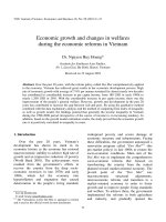
lated response of LNGDPC to Cholesky one
S.D. innovations of LNGFCF to GDP change
is almost double the accumulated response of
LNGDPC to Cholesky one S.D. innovations of
LNFDI. The period by period effect of TOP is
fluctuating, but the accumulated effect is positive (Figure 2).

GDP growth rates is mildly negative. Figure 1
further reveals that the initial positive shock
given to the capital formation raises economic
growth rates to its peak at approximately 0.45%
by the end of the second year or the beginning
of the third year. Figure 1 shows that the initial positive shock given to the FDI raises economic growth rates to its peak at approximately
0.25% by the end of the third year or the beginning of the fourth year. Figure 1, however,
unearths a positive but fluctuating and diminishing influence on changes in real GDP over
time. Overall, the impulse response function
traces positive influence of the response variables on the GDP growth rates of India.

In the context of varying causal links of
both GDP growth rates with macro variables,
VECM were applied and short run causal links
were explored using Variance decomposition.
Variance decomposition determines how much
of the k-step ahead forecast error variance of
a given variable is explained by innovations
to each explanatory variable. In practice, it is
usually observed that own series shocks most
of the (forecast) error variance of the series in
the VAR. Variance decomposition separates the

variation in an endogenous variable into the
component shocks to the VAR and provides

In our model it might be particularly interesting to analyze accumulated impulse responses. Accumulated impulse responses at
time horizon h are obtained by summing up all
impulse responses from 0 to h. The accumuJournal of Economics and Development

54

Vol. 17, No.3, December 2015


Figure 2: Accumulated Response of LNGDPC to Cholesky One S.D. Innovations

information about the relative importance of
each random innovation in affecting the variables in the VAR. The variance decomposition
results at the end of 6 periods are shown in Table 6. The columns provide the percentage of
the forecast variance due to each innovation in
the VAR framework, with each row adding up
to 100. The variance of GDP growth rates is
always caused by 100 per cent by itself in the

first year. In the second year, the GDP growth
variance is decomposed into its own variance
(80.26%) followed by level of capital formation (10.55%), FDI (6.81%) and TOP (2.37%).
However, in subsequent years, the share of
GDP growth rates remains constant to approximately 20% followed by the volume of FCF,
FDI and TOP contributing 55%, 20% and 5.37
% respectively. On the other hand, the share of

Table 6: Variance decomposition of LNGDPC
Period

S.E.

LNGDPC

LNFDI

LNGFCF

LNTOP

1

0.333442

100.0000

0.000000

0.000000

0.000000

2

0.411305

80.26422

6.810032

10.55620

2.369547

3

0.647142

33.55584

12.34254

53.10896

0.992661

4

0.779879

23.10689

18.88285

55.23035

2.779907

5

0.823224

20.75484

20.97238

55.08566

3.187121

6

0.856835

20.02519

19.53738

55.06589

5.371542

Journal of Economics and Development

55

Vol. 17, No.3, December 2015

adjustment from the short-run equilibrium to
the long-run equilibrium state. The results of
this study reveal short run causality from the
FDI, GFCF and TOP to economic growth. The
impulse response function traces the positive
influence of the response variables on the GDP
growth rates of India. Broadly it seems that the
volatility of GDP growth rates is mainly caused
by the level of GFCF and FDI variation, as it
always accounts for the major portion (above
75%) of the fluctuations. Trade openness, however, provides less importance, as compared
to the degree of capital formation and FDI, in
changing GDP growth rates. With the volume
of international capital and the magnitude of
capital formation, in general, being the robust
determinants of economic growth, it is expected that the government of India should provide
more emphasis on the above factors to increase
its economic growth.

trade openness in explaining the variation of
real GDP remains low but explains around a
stable 5%. Broadly it seems that the volatility
of GDP growth rates is mainly caused by the
level of GFCF and FDI variation, as it always
accounts for the major portion (above 75%) of
the fluctuations.
5. Concluding remarks
The present study is an attempt to explore

the linkages between FDI, GFCF, TOP and
GDP growth empirically in the context of India by analyzing time series data for the period 1980-2013. The study reveals that there is
a significant relationship between economic
growth and the macro variables under consideration. The results of the study reveals a
trong unidirectional causal flow from changes
in FDI, trade openness and capital formation
to the GDP growth rates of India. Empirical
results indicate a significant and high speed of
Acknowledgement:

The authors gratefully acknowledge the helpful and constructive comments of the anonymous referee. The
authors are responsible for any remaining errors.

Notes:
1. Broadly speaking a data series is said to be stationary if its mean and variance are constant (nonchanging) over time and the value of covariance between two time periods depends only on the distance
or lag between the two time periods and not on the actual time at which the covariance is computed.

References
Adhikary, B. K.(2011), ‘FDI, trade openness, capital formation, and economic growth in Bangladesh: a
linkage analysis’, International Journal of Business and Management, Vol. 6, No.1, pp. 16-28.
Aghion P. and Howitt P. (1992), ‘A Model of Growth through Creative Destruction’, Econometrica, Vol.
60, No.2, pp. 323-351.
Alguacil, M. Cuadros, A. and Orts, V. (2002),‘Foreign Direct Investment, Exports and Domestic Performance
in Mexico: a Causality Analysis’, Economic Letters, Vol.77, No.3, pp. 371-376.
Asiedu, E. (2002),‘On the determinants of foreign direct investment developing counties: Is Africa
different?’, World Development, Vol.30, No.1, pp.107-119.
Journal of Economics and Development

56

Vol. 17, No.3, December 2015


Awokuse, T. O.(2007), ‘Causality between exports, imports and economic growth: evidence from Transition
economies’, Economic Letters, Vol. 94, No.3, pp. 389-395.
Barro R. J. (1990), ‘Government Spending in a Simple Model of Endogenous Growth’, Journal of Political
Economy, Vol. 98, No.5, pp. S103-S125.
Barro, R.J. (1991),‘Economic growth in cross section of countries’, Quarterly Journal of Economics,
Vol.106, No.2, pp. 407-444.
Barro, R.J. and Sala-I-Martin, X. (1995),‘Capital mobility in neoclassical models of growth’, American
Economic Review, Vol. 85, No.1, pp. 103-115.
Ben-David, D. (1998), ‘Convergence Clubs and Subsistence Economies’, Journal of Development
Economics, Vol. 55, No.1, pp. 155-171.
Bhagwati, J.(1988), Protectionism, Cambridge, MA : MIT Press.
Bhat, K. S., Sundari, T.C.U., and Kumarasamy, D. (2004), ‘Causal nexus between foreign investment and
economic growth in India’, The Indian Journal of Economics, Vol. 85, No.337, pp. 171-185.
Blomstrom, M., Robert, E., Lipsey, R., and Mario, Z. (1996),‘Is fixed investment the key to economic
growth?’, Quarterly Journal of Economics, Vol.111, No.1, pp. 269-276.
Borensztein, E. J., Gregorio and Lee, J. W. (1995), ‘How does foreign direct investment affect economic
growth?’, NBER Working Paper 5057, National Bureau of Economic Research, Inc.
Bosworth, B., Collins, S. M., and Virmani, A.(2007), ‘Sources of growth in the Indian economy’, NBER
Working Paper No. 12901, National Bureau of Economic Research, Inc.
Chandra, A., and Thompson, E.(2000), ‘Does public infrastructure affect economic activity?: Evidence
from the rural interstate highway system’, Regional Science and Urban Economics, Vol. 30, No.3,
pp. 457-490.
Chou, Y. L. (1969), Statistical Analysts, Holt Rinehart and Winston, London.
Chuang, Y. (2002),‘The Trade-Induced Learning Effect on Growth: Cross-Country Evidence’, Journal of
Development Studies, Vol. 39, No.2, pp. 137–154
Chuang, Y. C. (2000),‘Human Capital, Exports, and Economic Growth: A Causality Analysis for Taiwan,
1952–1995’, Review of International Economics, Vol. 8, No. 4, pp. 712-720.

Collier, P. and Gunning, J.W. (1999), ‘Explaining African Economic Performance’, Journal of Economic
Literature, Vol. 37, No.1, pp. 64-111.
Dickey, D.A., and Fuller, W.A. (1981),‘Likelihood ratio statistics for autoregressive time series with a unit
root’, Econometrica, Vol. 49, No.4, pp. 1057-1072.
Ding, S., and Knight, J.(2011), ‘Why has China Grown So Fast? The Role of Physical and Human Capital
Formation’, Oxford Bulletin of Economics and Statistics, Vol. 73, No.2, pp.141-174.
Dritsaki, M., Dritsaki, C., and Adamopoulos, A. (2004), “A causal Relationship between Trade, Foreign
Direct Investment and Economic Growth for Greece’, American Journal of Applied Sciences, Vol.1,
No.3, pp. 230-235
Eberts, R. W. and Michael S. F.(1987), ‘Estimating the Relationship Between Local Public and Private
Investment’, Working Paper No. 8703, Federal Reserve Bank of Cleveland.
Engle, R.F. and Granger, C.W.J. (1987),‘Cointegration and error correction: representation, estimation, and
testing’, Econometrica, Vol. 55,No.2, pp. 251-276.
Feder, G. (1982),‘On exports and economic growth’, Journal of Development Economics, Vol.12, No.1-2,
pp. 59-73.
Findlay, R. (1978), ‘Relative backwardness, direct foreign investment, and the transfer of technology: a
simple dynamic model’, Quarterly Journal of Economics, Vol. 92, No.1, pp. 1–16.
Ghani, E., and Musleh-ud Din(2006), ‘The impact of public investment on economic growth in Pakistan’,
Journal of Economics and Development

57

Vol. 17, No.3, December 2015


The Pakistan Development Review, Vol. 45, No.1, pp. 87-98.
Ghura, D. and Hadjimichael, T. (1996), ‘Growth in Sub-Saharan Africa’, IMF Staff Papers, International
Monetary Fund.
Granger, C.W.J. (1969), ‘Investigating Causal Relations by Econometric Models and Cross-spectral
Methods’, Econometrica, Vol. 37, No.3, pp.24-36.

Granger, C.W.J. (1988), ‘Some recent developments in a concept of causality’, Journal of Econometrics,
Vol. 39, No.1-2, pp. 199-211.
Granger, C.W.J., and Newbold, P. (1974), ‘Spurious regressions in econometrics’, Journal of Econometrics,
Vol. 2, No.1, pp. 111-120.
Grossman G. and Helpman E. (1991), Innovation and Growth in the Global Economy, Cambridge: MIT
Press.
Hassan, A.(2007), ‘Exports and Economic Growth in Saudi Arabia: A VAR Model Analysis’, Journal of
Applied Sciences, Vol. 7, No.23, pp. 3649-3658.
Hermes, N., and Lensink, R. (2003), ‘Foreign direct Investment, Financial Development and Economic
Growth’, The Journal of Development Studies, Vol. 40, No.1, pp. 142-163.
Hernandez-Cata, E. (2000), ‘Raising Growth and Investment in Sub-Saharan Africa: What Can be Done?’,
Policy Discussion Paper: PDP/00/4, International Monetary Fund, Washington, D.C.
Ismail, S. (2012),‘Trade Induced Technology Spillover and Economic Growth: An Econometric Analysis’,
in the International Trade in Emerging Economies, ed. by Shahid Ahmed and Shahid Ashraf, New
Delhi: Bloomsbury.
Johansen, S. (1988),‘Statistical analysis of cointegration vectors’, Journal of Economic Dynamics and
Control, Vol.12, No.2-3, pp. 231-254.
Johansen, S. (1991), ‘Estimation and Hypothesis Testing of Cointegration Vectors in Gaussian Vector
Autoregressive Models’, Econometrica, Vol. 59, No.6, pp. 1551–1580.
Kendrick, J.W. (1993),‘How much does capital explain?’, In the Explaining Economic Growth. Essays in
Honour of Angus Maddison, ed. byA. Szirmai, B. Van Ark and D. Pilat, North Holland: Amsterdam.
Kim, Jong-Il and Lau, J. L.(1994), ‘The Sources of Economic Growth of the East Asian Newly Industrialized
Countries’, Journal of the Japanese and International Economies, Vol 8, No.3, pp. 235-271.
Konya, L. (2006), ‘Exports and growth: Granger causality Analysis on OECD countries with panel data
approach’, Economic Modelling, 23, No.6, pp. 978-992.
Kormendi, R. C., and Meguire, P. G. (1985), ‘Macroeconomic determinants of growth: Cross-country
evidence’, Journal of Monetary Economics, Vol. 16, No.2, pp. 141-163.
Krugman, P.R.(1984),‘Import protection as export promotion’, In the Monopolistic Competition in
International Trade, ed. by H. Kierzkowski, Oxford: Oxford University Press, UK.
Kumar, N., and Pradhan, J. P. (2002),‘FDI, externalities, and economic growth in developing countries:

Some empirical explorations and implications for WTO negotiations on investment’, RIS Discussion
Paper No. 27/2002, New Delhi, India.
Kwiatkowski, D., Phillips, P.C.B., Schmidt, P., and Shin, Y. (1992), ‘Testing the Null Hypothesis of
Stationary against the Alternative of a Unit Root’, Journal of Econometrics, Vol. 54, No.1-3, pp.
159-178.
Lensink, R.and Morrissey, O. (2006), ‘Foreign Direct Investment: Flows, Volatility, and the Impact on
Growth’, Review of International Economics, Vol. 14, No.3, pp. 478–493.
Levine, R., and Renelt, D. (1992), ‘A sensitivity analysis of cross-country regressions’, The American
Economic Review, Vol. 82, No. 4, pp. 942-963.
Lucas R. (1988), ‘On the Mechanics of Economic Development’, Journal of Monetary Economics, Vol. 22,
Journal of Economics and Development

58

Vol. 17, No.3, December 2015


No.1, pp. 3-42.
Marin, D. (1992), ‘Is the export-led growth hypothesis valid for industrialized countries?’, Review of
Economics and Statistics, Vol. 74, No.4, pp.678-688.
Massell, B.F., Pearson, S.R., and Fitch, J.B.(1972), ‘Foreign Exchange and Economic Development: An
Empirical Study of Selected Latin American Countries’, Review of Economics and Statistics, Vol.54,
No.2, pp. 208-212.
Michaely, M. (1977), ‘Exports and Growth: An Empirical Investigation’, Journal of Development
Economics, Vol.4, No.1, pp. 49-53.
Minford, P., Riley, J. and Nowell, E. (1995), ‘The Elixir of Growth: Trade, Non-traded Goods and
Development’, Centre for Economic Policy Research Discussion Paper No. 1165, London.
Munnell, A. H.(1992), ‘Policy watch: infrastructure investment and economic growth’, The Journal of
Economic Perspectives, Vol.6, No. 4, pp. 189-198.
Ndikumana, L. (2000), ‘Financial Determinants of Domestic Investment in Sub-Saharan Africa’, World

Development, Vol. 28, No. 2, pp. 381-400.
Parkinson, J. M. (1987), ‘The EMH and the CAPM on the Nairobi Stock Exchange’, East African Economic
Review, Vol. 13, No.2, pp. 105-110.
Paugel, A. T. (2007), International Economics, McGrawHill Irwin: New York.
Phillips, P.C.B., and Perron, P. (1988), ‘Testing for a unit root in time series regressions’, Biometrica, Vol.
LXXV, No. 2, pp. 335-346.
Prasad, E. S., Raghuram, G. R., and Subramanian, A. (2007), ‘Foreign capital and economic growth’,
NBER Working Papers 13619, National Bureau of Economic Research, Inc.
Ramos, F.F. (2001), ‘Exports, imports and economic growth in Portugal: Evidence from causality and
Cointegration Analysis’, Economic Modelling, Vol. 18, No. 4, pp. 613-623.
Robertson, D.H (1938), ‘The Future of International Trade’, Economic Journal, Vol. 48, No. 189, pp.1-14.
Romer P. (1986), ‘Increasing Returns and Long Run Growth’, Journal of Political Economy, Vol. 94, No.
5, pp. 1002-1037.
Romer P. (1990), ‘Endogenous Technological Change’, Journal of Political Economy, Vol. 98, No.5, pp.
S71- S102.
Sachs, J. D. and Warner, A. (1995), ‘Economic Reform and the Process of Global Integration’, Brookings
Papers on Economic Activity, No. 1, pp. 1-118.
Sahoo, P., Dash, R.K. and Nataraj, G., (2010), ‘Infrastructure development and economic growth in China’,
IDE Discussion Papers 261, Institute of Developing Economies, Japan External Trade Organization
(JETRO).
Salvatore, D. (1983), ‘A Simultaneous Equations Model of Trade and Development with Dynamic Policy
Simulations’, Kyklos, Vol. 36, No.1, pp. 66-90.
Thornton, J. (1996), ‘Cointegration, causality and export-led growth in Mexico’, Economic Letters, Vol.50,
No.3, pp. 413-416.
Tyler, W.G. (1981), ‘Growth and Export Expansion in Developing Countries: Some Empirical Evidence’,
Journal of Development Economics, Vol. 9, No.1, pp.121-130.
Voivodas, C. (1973),‘Exports, Foreign Capital Inflow and Economic Growth’, Journal of International
Economics’, Vol.3, No.4, pp. 337- 349.
Wang, E. C.(2002), ‘Public infrastructure and economic growth: a new approach applied to East Asian
economies’, Journal of Policy Modeling, Vol.24, No.5, pp. 411-435.

Zhang, K. H.(2001), ‘Does foreign direct investment promote economic growth? Evidence from East Asia
and Latin America’, Contemporary economic policy, Vol. 19, No. 2, pp. 175-185.
Journal of Economics and Development

59

Vol. 17, No.3, December 2015