Ebook Economics for business and management: Part 2
Bạn đang xem bản rút gọn của tài liệu. Xem và tải ngay bản đầy đủ của tài liệu tại đây (9.35 MB, 388 trang )
www.downloadslide.com
Chapter 10
Government policies: instruments and
objectives
Introduction
This chapter takes forward the broad analysis of Chapter 9 into the more specific
areas of government policy making. Such policies play a key role in shaping the macroenvironment in which businesses and households must operate. Government policies
on tax rates and allowances, levels and types of expenditure, interest rates and credit
availability, public service provision, pension entitlement and on many other issues
will have a major impact on businesses and households.
This chapter introduces the aggregate demand and aggregate supply schedules to
help deepen our understanding of issues such as inflation, unemployment and economic
growth.
Learning objectives:
By the end of this chapter you should be able to:
■
identify the key policy instruments available to governments in seeking to influence the macroeconomic environment and review their relative effectiveness
■
consider in some detail fiscal policy, monetary policy and exchange rate policy
in the UK and other economies and assess their impacts on businesses and
households
■
explain what is meant by ‘built-in stabilisers’ and show how these can help avoid
excessive increases or decreases in economic activity
■
understand how and why governments seek simultaneously to achieve the
objective of price stability, low unemployment, balance of payments equilibrium
and sustained economic growth and the implications for business and households
■
use aggregate demand and aggregate supply curves to analyse issues involving
inflation, unemployment and economic growth.
www.downloadslide.com
370 Chapter 10 · Government policies: instruments and objectives
We begin by looking in some detail at the use by governments of fiscal policy, paying
particular attention to its role in the UK.
Fiscal policy
‘Fiscal policy’ is the name given to government policies which seek to influence
government revenue (taxation) and or government expenditure. We have already seen
how changes in either can influence the equilibrium level of national income, with
implications for output, employment and inflation.
Major changes in fiscal policy in the UK are normally announced at the time of the
Budget, which in the UK traditionally takes place just before the end of the tax year on
5 April. Both revenue raising and expenditure plans are presented together at the Budget.
■ Budget terminology
A number of terms are often used to describe a Budget.
■
Budget deficit. When tax revenues fall short of public expenditure (T ` G).
■
Budget surplus. When tax revenue exceeds public expenditure (T p G).
■
Balanced budget. When tax revenue equals public expenditure (T # G).
Similarly, a number of terms are often used to describe the consequences of these
budget situations.
Watch out!
■
Public sector borrowing requirements (PSBR). Until recently, this term has been
widely used to describe the outcome of a budget deficit, since the government will
have to borrow to cover the excess of government spending over tax revenue
(G p T), at least in the short run. This borrowing may involve issuing government
bills and bonds to the financial markets.
■
Public sector net cash requirement (PSNCR). In recent years this has been the term
more usually used in the UK to refer to situations previously described by the PSBR.
The PSNCR is sometimes described as the public sector net borrowing requirement
(PSNBR).
■ Fiscal ‘rules’
Further terms are often used in seeking to describe the government’s fiscal policy.
For example, in 1998 the Labour government committed itself to the following two
important ‘fiscal rules’.
www.downloadslide.com
Taxation 371
■
The ‘golden rule’: over the economic cycle the government will only borrow to
invest and will not borrow to fund current expenditure. In effect the ‘golden rule’
implies that current expenditure will be covered by current revenue over the
economic cycle. Put another way, any borrowing to cover the PSNCR (public sector
net cash requirement) must be used only for investment purposes, in effect for
spending on infrastructure, such as roads and railways, capital equipment and so
on.
The ‘public debt rule’: over the economic cycle the ratio of public debt to
national income will be held at a ‘stable and prudent’ level. The ‘public debt rule’ is
rather less clear in that the phrase ‘stable and prudent’ is somewhat ambiguous.
However, taken together with the ‘golden rule’ it essentially means that, as an
average over the economic cycle, the ratio of PSNCR to national income cannot
exceed the ratio of investment to national income. Given that, historically, government investment has been no more than 2% to 3% of national income, then clearly
the PSNCR as a percentage of national income must be kept within strict limits.
■
Checkpoint 1
What do you think is meant by the ‘economic cycle’?
It will be useful to consider government taxation and government expenditure in turn
and consider their impacts on businesses and households.
Taxation
Taxation is the major source of government revenue, with a ‘tax’ being a compulsory
charge laid down by government. You must remember that the government is spending your money; it has no money of its own. Apart from government borrowing, it
only has the money which it generates from taxation. Don’t forget that everyone pays
taxes. Even those who do not work pay expenditure taxes (e.g. VAT).
Example:
Taxation in various economies
It is often said that the UK is overtaxed. Currently around 38% of all UK
national income is taken in various forms of taxation, which actually places the
UK as only a middle-ranked country in terms of tax burden. Of the 20 largest
world economies, ten have a higher tax burden than the UK. For example, over
53% of national income is taken in tax in Sweden, 49% in Denmark, 46% in
Austria, 45% in Belgium, Norway and Finland, though only around 30% in the
US.
www.downloadslide.com
372 Chapter 10 · Government policies: instruments and objectives
■ Types of taxation
As long ago as the eighteenth century, Adam Smith laid down the rules for a ‘good tax’
in his so-called ‘canons of taxation’. A tax should be:
1 equitable (fair); those who can afford to pay more should do so;
2 economic; more should be collected in tax than is needed to cover the costs of
administration;
3 transparent; individuals should know how much tax they are paying;
4 convenient; the taxpayer should not find it difficult to pay the tax.
Direct and indirect taxes
Taxes are often grouped under these headings depending on the administrative
arrangements for their collection.
■
Direct taxes. These taxes are paid directly to the Exchequer by the taxpayer, whether
by individuals (e.g. Income Tax, Employee’s National Insurance, Capital Gains Tax)
or by companies (e.g. Corporation Tax, Employer’s National Insurance). Most of
the revenue from direct taxes comes from taxing the income of the individuals and
companies.
■
Indirect taxes. These taxes are paid indirectly to the Exchequer by the taxpayer, e.g.
via retailers. Other indirect taxes include a range of excise duties (on oil, tobacco
and cars) and import duties. Most of the revenue from indirect taxes comes from
taxing the expenditure of individuals and companies.
Table 10.1 Types of tax: % of tax revenue in 2003
Direct taxes
Income Tax
National Insurance (Employers ! Employees)
Corporation Tax
Capital Gains, Inheritance
Total Direct
Indirect tax
VAT
Fuel duties
Tobacco
Alcohol
Other indirect
Total Indirect
% of total tax revenue
29%
16%
7%
3%
55%
% of total tax revenue
16%
6%
2%
2%
2%
28%
Table 10.1 shows that direct taxes contribute some 55% of total tax revenue, when we
include employers’ and employees’ National Insurance Contributions, corporation
taxes on company profits and capital gains and inheritance taxes. Indirect taxes
www.downloadslide.com
Taxation 373
contribute some 28% of total tax revenues, with VAT the most important of these,
and ‘other taxes’ (e.g. council tax, Business rates etc.) make up the other 17%.
There is a danger in discussing tax issues to forget that households and businesses
are affected by tax in general (via the circular flow) and sometimes by taxes in particular. Some 30 years of VAT in the UK has had different implications for Blackpool
Pleasure Beach and United Biscuits, as is indicated in the example below.
Example:
VAT, Blackpool Pleasure Beach and United Biscuits
VAT was invented in 1965 by Maurice Laure, a French civil servant, for use in
the then European Common Market. The UK adopted the system in 1973.
Because VAT is not supposed to be levied on ‘essential’ products but only on
‘luxuries’, various businesses have sought to be VAT exempt, sometimes with
controversial results (e.g. cakes are VAT exempt, biscuits are not).
In 1974 Blackpool Pleasure Beach brought one of the first claims against
Britain’s new tax. They said their Big Dipper rollercoaster was a form of transport
(VAT exempt) and argued that passengers should therefore be exempt from VAT.
Customs and excise didn’t agree. United Biscuits got into a wrangle with the
authorities when it claimed its Jaffa Cakes snacks were cakes and not biscuits,
thereby making them exempt from VAT. After taking the case to a tribunal the
company won.
Total revenues since the introduction of VAT in 1973 add up to £826bn. The
annual revenue for this tax in 2004 was around £645bn, up from £2.5bn in
1973. At 25% Denmark and Sweden have the highest VAT rates in Europe.
At the end of this section (p. 376) we look in more detail at the advantages and disadvantages of both direct and indirect taxation.
Specific and percentage taxes
■
Specific tax. This is expressed as an absolute sum of money per unit of the product
and is sometimes called a ‘lump-sum’ tax. Excise duties are often of this kind, being
so many pence per packet of cigarettes or per proof of spirit or per litre of petrol.
■
LINKS
Chapter 2 (p. 56) looks at the
impact of specific (lump-sum)
and percentage taxes on
business costs and supply
curves.
Percentage tax. This is levied not on volume but on value; e.g. in the
UK in 2004 5 VAT was 17.5% of sales price, and corporation tax
was 30% of assessable profits for larger companies and 19% of
assessable profits for smaller companies. These percentage taxes are
sometimes called ad valorem (to vary) since the absolute sum of
money paid per unit of the product varies with the price.
Progressive and regressive taxes
■
Progressive taxes. These occur when, as incomes rise, the proportion of total
income paid in tax rises. Income tax is progressive, partly because of allowances for
low-paid workers before any tax is paid, and partly because tax rates rise for higher
income groups.
www.downloadslide.com
374 Chapter 10 · Government policies: instruments and objectives
■
Regressive taxes. These occur when, as incomes rise, the proportion of total income
paid in tax falls. VAT is regressive, since the same absolute amount is paid by rich
and poor alike, which means that for those on higher incomes a lower proportion
of higher incomes is paid in VAT and most other indirect taxes.
■
Proportional taxes. These occur when, as incomes rise, the proportion of total
income paid in tax remains unchanged.
Those who suggest that more tax revenue should come from indirect taxes on expenditure are, according to this analysis, supporting a more regressive tax regime.
Hypothecated taxes
A recent approach favoured by many as a means of raising the tax take, whilst retaining
public support, involves the idea of hypothecation. This is the allocation of monies
received from current or additional taxes to specific spending outcomes.
■ Individual taxes
Here we consider some of the different taxes in a little more detail.
Income tax in the UK
Not all income is taxed; everyone is allowed to earn a certain amount before paying
tax, which is shown in the tax code. For example, in 2004 5 each single person in the
UK under 65 years had a tax allowance of £4,745 before tax.
Most workers have their tax paid for them by their employer using PAYE (Pay As
You Earn). This conforms to the third and fourth ‘canons of taxation’, namely that
taxes should be transparent and convenient. Employers have to give the worker a
salary advice form showing the amount of tax deducted for the current time period (a
week or a month) and the amount of accumulated tax deducted in the current tax year.
Table 10.2 shows how UK income tax rates have been simplified and lowered in the
16 years from 1987 8 to 2004 5.
Table 10.2 UK income tax schedules 1987 8 and 2004 5
Rate of tax (%)
1987 8 Taxable income
(£)
2004 5 Taxable income
(£)
10
22
27
40
45
50
55
60
–
–
0–17,900
17,901–20,400
20,401–25,400
25,401–33,300
33,301–41,200
over 41,200
0–1,960
1,961–30,500
over 30,500
–
–
–
–
www.downloadslide.com
Taxation 375
Other direct taxes in the UK
■
National Insurance. A tax on employment, paid by both employees and employers.
In 2004 5 this is levied at 0% on employees earning up to £91 per week, rising
sharply to 11% on earnings between £91 and £610 per week, but only 1% on
additional earnings over £610 per week.
■
Capital Gains Tax. A tax on the increased value of an asset when it is sold. Capital
gains above £7,790 are taxable at rates rising from 10% to 40%.
■
Inheritance Tax. A tax on inheritance or gifts. In 2004 5 inheritance tax at a rate of
40% is only paid on estates valued at over £263,000.
■
Corporation Tax. A tax on company profits at 30% as the standard rate, but a
lower 19% for small firms.
Indirect taxes in the UK
■
Value Added Tax (VAT). A tax on expenditure on most goods and services (currently
17.5% in the UK). Some items (e.g. children’s clothes) are VAT exempt. VAT is a tax
on expenditure levied by all EU countries, though at different rates.
■
Excise duties. A specific tax of an absolute amount levied at different rates on goods
such as tobacco, petrol, alcohol.
Other taxes in the UK
Some UK taxes are difficult to define or put into neat categories, such as the BBC
licence; Road Fund Licence; Council Tax; Stamp Duty; Airport Tax; fees paid by local
residents to the council for parking; prescription charges.
Checkpoint 2
1 Use either the W J diagram or the 45° diagram to show how each of the following might
influence the national income:
(a) a 1% rise in the basic rate of income tax;
(b) a £1 increase per item in a specific tax (e.g. excise duty).
2 Would either of these extra taxes influence the national income multiplier?
Taxes and economic incentives
There is an ongoing debate as to whether or not taxes are ‘excessive’ in the UK and
whether current tax rates act as a disincentive to UK households and businesses.
Taxes and incentives to work
Many empirical studies have been conducted on tax rates and incentives, with no clear
results. However, one widely accepted approach does warn governments against
imposing too high an overall tax rate.
Laffer curve
Professor Laffer derived a relationship between tax revenue and tax rates of the form
shown in Figure 10.1. The curve was the result of econometric techniques, through
which a ‘least square line’ was fitted to past US observations of tax revenue and tax
rate. The dotted line indicates the extension of the fitted relationship (continuous) line,
www.downloadslide.com
376 Chapter 10 · Government policies: instruments and objectives
Tax revenue
as there will tend to be zero tax revenue at both 0% and 100% tax rates. Tax
revenue # tax rate " output (income), so that a 0% tax rate yields zero tax revenue,
whatever the level of output. A 100% tax rate is assumed to discourage all output,
except that for subsistence, again yielding zero tax revenue. Tax revenue must reach a
maximum at some intermediate tax rate between these extremes.
45%
O
60%
100%
Tax rate
(overall)
Fig 10.1 The ‘Laffer’ curve
LINKS
Our indifference analysis of Appendix 1
introduced the ideas of ‘income’ and
‘substitution’ effects. A higher tax on income will
have two effects, which pull in opposite
directions.
■
■
An ‘income effect’, with real income reduced
via higher taxes, which means less
consumption of all items, including leisure,
i.e. more work is performed.
A ‘substitution effect’, with leisure now
cheaper via higher taxes, since less real
income is now sacrificed for each unit of
leisure consumed. The substitution effect
leads to cheaper leisure being substituted for
work, i.e. less work.
On grounds of theory alone we cannot tell which
effect will be the stronger, i.e. whether higher
taxes on income will raise or lower the time
devoted to work rather than leisure (where, of
course, the worker has some choice).
The London Business School has estimated a Laffer
curve for the UK using past data. Tax revenue was
found to reach a peak at around a 60% ‘composite tax
rate’, i.e. one which includes both direct and indirect
taxes, as well as various social security payments, all
expressed as a percentage of GDP. If the composite tax
rate rises above 60%, then the disincentive effect on
output is so strong (i.e. output falls so much) that tax
revenue (tax rate " output) actually falls, despite the
higher tax rate.
The Laffer curve in fact begins to flatten out at
around a 45% composite tax rate. In other words, as
the overall tax rate rises to about 45%, the disincentive
effect on output is strong enough to mean that little
extra tax revenue results. Econometric studies of this
type have given support to those in favour of limiting
overall rates of tax. In fact the reduction in the top
income tax rate to 40% in the UK in 1988 9 was
inspired by the Laffer curve.
■ Direct versus indirect taxes
It might be useful to consider in more detail the advantages and disadvantages of direct
and indirect systems of taxation. For convenience we shall compare the systems under
four main headings, with indirect taxes considered first in each case.
www.downloadslide.com
Taxation 377
Macroeconomic management
Indirect taxes can be varied more quickly and easily, taking more immediate effect,
than can direct taxes. Since the Finance Act of 1961, the Chancellor of the Exchequer
has had the power (via ‘the regulator’) to vary the rates of indirect taxation at any time
between Budgets. Excise and import duties can be varied by up to 10%, and VAT by
up to 25% (i.e. between 13.13% and 21.87% for a 17.5% rate of VAT). In contrast
direct taxes can only be changed at Budget time. In the case of income tax, any change
involves time-consuming revisions to PAYE codings. For these reasons, indirect taxes
are usually regarded as a more flexible instrument of macroeconomic policy.
Economic incentives
We have already seen how, in both theory and practice, direct taxes on income affect
incentives to work. We found that neither in theory nor in practice need the net effect
be one of disincentive. Nevertheless, it is often argued that if the same sum were
derived from indirect taxation, then any net disincentive effect that did occur would be
that much smaller. In particular, it is often said that indirect taxes are less visible (than
direct), being to some extent hidden in the quoted price of the product. However,
others suggest that consumers are well aware of the impact of indirect taxes on the
price level. Certainly for products with relatively inelastic demands (Chapter 2, p. 57)
any higher indirect taxes will be passed on to consumers as higher prices, and will
therefore not be less visible than extra direct taxation.
Economic welfare
It is sometimes argued that indirect taxes are, in welfare terms, preferable to direct
taxes, as they leave the taxpayer free to make a choice. The individual can, for
instance, avoid the tax by choosing not to consume the taxed commodity. Although
this ‘voluntary’ aspect of indirect taxes may apply to a particular individual and a
particular tax, it cannot apply to all individuals and all taxes. In other words, indirect
taxes cannot be ‘voluntary’ for the community as a whole. If a chancellor is to raise a
given sum through a system of indirect taxes, individual choices not to consume taxed
items must, if widespread, be countered either by raising rates of tax or by extending
the range of goods and services taxed.
Another argument used to support indirect taxes on welfare grounds is that they
can be used to combat ‘externalities’. In Chapter 8 we noted that an externality occurs
where private and social costs diverge. Where private costs of production are below
social costs, an indirect tax could be imposed, or increased, so that price is raised to
reflect the true social costs of production. Taxes on alcohol and tobacco could be
justified on these grounds. By discriminating between different goods and services,
indirect taxes can help reallocate resources in a way that raises economic welfare for
society as a whole.
On the other hand, indirect taxes have also been criticised on welfare grounds for
being regressive, the element of indirect tax embodied in product prices taking a higher
proportion of the income from lower-paid groups. Nor is it easy to correct for this. It
would be impossible administratively to place a higher tax on a given item for those
with higher incomes, although one could impose indirect taxes mainly on the goods
and services consumed by higher-income groups, and perhaps at higher rates.
www.downloadslide.com
378 Chapter 10 · Government policies: instruments and objectives
In terms of economic welfare, as in terms of economic incentives, the picture is
again unclear. A case can be made, with some conviction, both for and against direct
and indirect taxes in terms of economic welfare.
Administrative costs
Indirect taxes are often easy and cheap to administer. They are paid by manufacturers
and traders, which are obviously fewer in number than the total of individuals paying
income tax. This makes indirect taxes such as excise and import duties much cheaper
to collect than direct taxes, though the difference is less marked for VAT, which
requires the authorities to deal with a large number of mainly smaller traders.
Even if indirect taxes do impose smaller administrative costs than direct taxes for a
given revenue yield, not too much should be made of this. It is, for instance, always
possible to reform the system of PAYE and reduce administrative costs; for example,
the computerisation of Inland Revenue operations may, in the long run, significantly
reduce the administrative costs associated with the collection of direct taxes.
In summary, there is no clear case for one type of tax system compared to another.
The macroeconomic management and administrative cost grounds may appear to
favour indirect taxes, though the comparison is only with the current system of direct
taxation. That system can, of course, be changed to accommodate criticisms along
these lines. On perhaps the more important grounds of economic incentives and
economic welfare the case is very mixed, with arguments for and against each type of
tax finely balanced.
Government expenditure
Government expenditure was almost 49% of national income in the UK in 1981, but
in 2004 it had fallen to around 41% of national income. However, major increases in
government spending over the period 2003–05 were announced in the Comprehensive
Spending Review of November 2002, raising the projected ratio of government
spending to over 42% of national income by 2005 6.
Table 10.3 gives a broad breakdown of the share of various departments and
programmes in UK total government spending in 2003 4.
Clearly, Social Security, Health and Education are the key spending areas, taking
around 56% of all government expenditure. The impact on business of extra government spending will depend on the sectors in which the money is spent. Obviously,
defence contractors will benefit directly from extra spending on the armed services.
However, as we noted in Chapter 9 (p. 354), the ‘multiplier effect’ from the extra
government spending will increase output, employment, income and spending
indirectly in many sectors of economic activity.
We have already considered (p. 371) the various ‘rules’ the Labour government has
established for broadly controlling the growth of government expenditure over the
economic cycle. Given the criticism that is often made of allegedly ‘excessive’ government spending in the UK, it is interesting to note that the UK is below average on most
cross-country indices of government spending.
www.downloadslide.com
Government expenditure 379
Table 10.3 UK government expenditure:
% shares in 2003 4
Example:
Department Programme
%
Social Security
Health
Education
Debt interest
Defence
Law and order
Industry and employment
Housing environment
Transport
Contributions to EU
Overseas aid
Other
28
17
11
7
6
6
4
3
2
1
0.5
5
Government spending in various economies
Although the UK government is sometimes criticised for excessive spending, at
41% of national income, government spending is less than the 44% average
across the EU countries, but more than the 31% of national income recorded for
government spending in the US. In fact, in 2003, out of 14 major countries, the
UK was only tenth highest in terms of the share of national income given to
government expenditure.
■ Case for controlling public expenditure
The arguments used by those in favour of restricting public expenditure include the
following.
More freedom and choice
The suggestion here is that excessive government expenditure adversely affects
individual freedom and choice.
■
First, it is feared that it spoonfeeds individuals, taking away the incentive for
personal provision, as with private insurance for sickness or old age.
■
Second, that by impeding the market mechanism it may restrict consumer choice.
For instance, the state may provide goods and services that are in little demand,
whilst discouraging others (via taxation) that might otherwise have been bought.
■
Third, it has been suggested that government provision may encourage an unhelpful
separation between payment and cost in the minds of consumers. With government
provision, the good or service may be free or subsidised, so that the amount paid by
the consumer will understate the true cost (higher taxes etc.) of providing him or her
with that good or service, thereby encouraging excessive consumption of the item.
www.downloadslide.com
380 Chapter 10 · Government policies: instruments and objectives
Crowding out the private sector
The previous Conservative government had long believed that (excessive) public
expenditure was at the heart of Britain’s economic difficulties. It regarded the private
sector as the source of wealth creation, part of which was being used to subsidise the
public sector. Sir Keith Joseph clarified this view during the 1970s by alleging that ‘a
wealth-creating sector which accounts for one-third of the national product carries on
its back a State subsidised sector which accounts for two-thirds. The rider is twice as
heavy as the horse.’
Bacon and Eltis (1978) attempted to give substance to this view. They suggested
that public expenditure growth had led to a transfer of productive resources from the
private sector to a public sector producing largely non-marketed output and that this
had been a major factor in the UK’s poor performance in the post-war period. Bacon
and Eltis noted that public sector employment had increased by some 26%, from 5.8
million workers to 7.3 million, between 1960 and 1978, a time when total employment was being squeezed by higher taxes to finance this growth in the public sector –
the result being deindustrialisation, low labour productivity, low economic growth
and balance of payments problems.
Control of money
Another argument used by those who favour restricting public expenditure is that it
must be cut in order to limit the growth of money supply (see p. 387) and to curb inflation. The argument is that a high PSBR (now PSNCR – public sector net cash requirement), following public expenditure growth, must be funded by the issue of Treasury
bills and government stock, which increase liquidity in the system and can lead to a
multiple expansion of bank deposits (money), with perhaps inflationary consequences.
A related argument is that public expenditure must be restricted, not only to limit
the supply of money, but also its ‘price’ – the rate of interest. The suggestion here is
that to sell the extra bills and bonds to fund a budget deficit, interest rates must rise to
attract investors. This then puts pressure on private sector borrowing with the rise
in interest rates inhibiting private sector investment and investment-led growth. A
major policy aim of governments has, therefore, often been to control public sector
borrowing.
Incentives to work, save and take risks
There are also worries that increased public spending not only pushes up government
borrowing, but also leads to higher taxes, thereby reducing the incentives to work,
save and take risks. However, we have already noted that the evidence to support the
general proposition that higher taxes undermine the work ethic is largely inconclusive.
Balance of payments stability
A further line of attack has been that the growth of public expenditure may create
problems for the balance of payments (see p. 407). The common sense of this argument is that higher public spending raises interest rates and attracts capital inflow,
which in turn raise the demand for sterling and therefore the exchange rate. A higher
pound then makes exports dearer and imports cheaper so that the balance of payments
deteriorates.
www.downloadslide.com
Fiscal policy and stabilisation 381
The debate on the role of public expenditure continues. However, the present
government has placed great emphasis on containing such expenditure by setting out
its ‘fiscal rules’, which we considered earlier (p. 371).
Checkpoint 3
1 Use either the W J diagram or the 45° diagram to show how a major increase in government expenditure might influence the equilibrium level of national income.
2 Can you suggest any other possible consequences from such an increase in government
expenditure?
Fiscal policy and stabilisation
■ Business cycle
The terms business cycle or trade cycle are often used to refer to the tendency for
economies to move from economic boom into economic recession, or vice versa.
Economic historians have claimed to observe a five- to eight-year cycle of economic
activity between successive peaks (A,C) or successive troughs (B,D) around a general
upward trend (T) of the type shown in Figure 10.2.
T
GDP
C
A
D
B
O
Time
Fig 10.2 Business (trade) cycle
From a business perspective it is clearly important to be aware of such a business cycle,
since investment in extra capacity in boom year A might be problematic if demand had
fallen relative to trend by the time the capacity came on stream in the recession year B.
Example:
Microchip manufacture
In the boom dot.com years of the late 1990s many of the major chip-making
firms such as Intel, Samsung, Fujitsu and Siemens invested in extra chip-making
plants. Unfortunately, by the time many of these were ready for operation, the
dot.com boom had turned to bust and many of these state-of-the-art plants had
to be closed when excess chip supply resulted in plunging prices.
www.downloadslide.com
382 Chapter 10 · Government policies: instruments and objectives
From a business perspective, investment might be better timed to take place at or
around points B or D in Figure 10.2, depending on the time lags involved. Even better
would be a situation in which government fiscal policies had ‘smoothed’ or stabilised
the business cycle around the trend value (T) by making use of ‘built-in’ stabilisers or
by using ‘discretionary’ fiscal policy. It is to this policy objective that we now turn.
■ Built-in stabilisation
Some of the tax and spending programmes we have discussed will act as built-in (or
automatic) stabilisers. They do this in at least two ways.
■
Bringing about an automatic rise in withdrawals and or fall in injections in times of
‘boom’. For example, when the economy is growing rapidly, individual incomes,
business incomes and spending on goods and services will all be rising in value,
thereby increasing the government’s revenue from both direct and indirect taxes. At
the same time, unemployment is likely to be falling, reducing the government’s
spending on social security, unemployment and other benefits.
This ‘automatic’ rise in withdrawals and reduction in injections will help to
dampen any excessive growth in national income which might otherwise result in
rapid inflation and unsustainable ‘boom’ conditions.
■
Bringing about an automatic fall in withdrawals and or rise in injections in times of
recession. For example, when the economy is contracting, individual incomes,
business incomes and spending on goods and services will all be falling in value,
thereby reducing the government’s tax revenue from both direct and indirect taxes.
At the same time, unemployment is likely to be rising, increasing the government’s
spending on social security, unemployment and other benefits.
This ‘automatic’ fall in withdrawals and rise in injections will help to stimulate
the economy and prevent national income from falling as far as it otherwise might
have done.
Checkpoint 4
How can the government use fiscal policy to increase the extent of built-in (automatic)
stability in the economy?
■ Discretionary stabilisation
On occasions, governments will intervene in the economy for specific purposes, such
as reinforcing the built-in stabilisers already described.
■
If an ‘inflationary gap’ is identified (Chapter 9, p. 359) then the government may
seek to reduce G or raise T to eliminate it.
■
If a ‘deflationary gap’ is identified (Chapter 9, p. 360) then the government may
seek to raise G or reduce T to close it.
www.downloadslide.com
Fiscal policy and stabilisation 383
These are examples of discretionary fiscal policy, where the government makes a
conscious decision to change its spending or taxation policy. As compared to built-in
stabilisers, discretionary fiscal stabilisation policy faces a number of difficulties.
Time lags
At least two time lags can be identified.
■
Recognition lag. It takes time for the government to collect and analyse data, recognise any problem that may exist, and then decide what government spending and
taxation decisions to take.
■
Execution lag. Having made its fiscal policy decisions, it takes time to implement
these changes and it also takes time for these changes to have an effect on the
economy.
Actual output (Y) minus full employment output (YF)
(Government spending minus tax revenue)
In terms of discretionary fiscal policy these time lags can result in the government
reinforcing the business cycle, rather than stabilising it, as indicated in Figure 10.3.
Economic cycle
boom
boom
0
1
2
3
recession
4
5
6
7
8
Time
recession
Discretionary fiscal policy (no time lags)
Discretionary fiscal policy (2 period time lag)
Fig 10.3 Stabilisation of the business cycle and discretionary fiscal policy
■
The business (trade) cycle is shown as a continuous line in the diagram, with a complete cycle (peak to peak) lasting four time periods. For the business cycle the relevant variable on the vertical axis is ‘Actual output (Y) minus full employment
output’ (Y F).
– Where this is positive, as in time periods 1 and 2, we have our familiar ‘inflationary gap’ (since Y p Y F).
– Where this is negative, as in time periods 3 and 4, we have our familiar ‘deflationary gap’ (since Y ` Y F)
www.downloadslide.com
384 Chapter 10 · Government policies: instruments and objectives
■
Discretionary fiscal policy is shown as both a coloured continuous line (no time lag)
and a dotted line (two-period time lag) in the diagram. For discretionary fiscal policy
the relevant variable on the vertical axis is ‘Government spending minus tax revenue’.
– Where the business cycle is experiencing an ‘inflationary gap’ (time periods 1
and 2), the appropriate discretionary fiscal policy is a budget surplus (G ` T).
This is the case with the coloured continuous line.
– Where the business cycle is experiencing a ‘deflationary gap’ (time periods 3 and
4), the appropriate discretionary fiscal policy is a budget deficit (G p T). This is
again the case with the coloured continuous line.
If the timing of the discretionary fiscal policy is correct, as with the coloured continuous line (no time lag), then intervention by the government will help to ‘stabilise’ the
business cycle, with discretionary fiscal policy resulting in a net withdrawal in times of
‘boom’ and a net injection in times of recession.
However, when the recognition and execution time lags are present, discretionary
fiscal policy can actually turn out to be ‘destabilising’. This is the case in Figure 10.3 if
these time lags cause a two-time-period delay in discretionary fiscal policy coming into
effect. The dotted line of Figure 10.3 shows government intervention resulting in a
budget surplus at times of recession (time periods 3 and 4) and a budget deficit at times
of boom (time periods 5 and 6). This is exactly the opposite of what is needed for a
discretionary fiscal policy to help stabilise the business cycle.
Checkpoint 5
Why might an inaccurate estimate of the national income multiplier by government also
pose a problem for the use of discretionary fiscal policy?
Although fiscal policy is widely regarded as the most important policy approach in
the UK, monetary policy can also have important impacts on national income and
therefore on the prospects for businesses and households.
Monetary policy
Monetary policy has been defined as the attempt by government to manipulate the
supply of, or demand for, money in order to achieve specific objectives. Since the rate
of interest has an important role in determining the demand for money, monetary
policy often concentrates on two key variables:
■
money supply;
■
rate of interest.
■ Money supply
If government is to control the money supply it must know what money is!
www.downloadslide.com
Monetary policy 385
Definition of money
This may seem obvious but in a modern economy it is not. Money has been defined as
anything that is generally acceptable in exchange for goods and services or in settlement of debts. Box 10.1 looks at the functions which an asset must fulfil if it is to be
regarded as ‘money’.
Box 10.1
What is money?
There are four key functions which money performs.
1 To act as a medium of exchange or means of payment. Money is unique in performing this
function, since it is the only asset which is universally acceptable in exchange for goods
and services. In the absence of a medium of exchange, trade could only take place if there
was a double coincidence of wants; in other words, only if two people had mutually acceptable commodities to exchange. (I want yours, you want mine.) Trade of this type takes
place on the basis of barter.
Clearly barter would restrict the growth of trade. It would also severely limit the extent
to which individuals were able to specialise. By acting as a medium of exchange money
therefore promotes specialisation. A person can exchange his her labour for money, and
then use that money to purchase the output produced by others. We have seen in
Chapter 3 that specialisation greatly increases the wealth of the community. By acting as a
medium of exchange money is therefore fulfilling a crucial function, enhancing trade,
specialisation and wealth creation.
2 To act as a unit of account. By acting as a medium of exchange, money also provides a
means of expressing value. The prices quoted for goods and services reflect their relative
value and in this way money acts as a unit of account.
3 To act as a store of wealth. Because money can be exchanged immediately for goods and
services it is a convenient way of holding wealth until goods and services are required. In
this sense money acts as a store of wealth.
4 To act as a standard for deferred payment. In the modern world, goods and services are
often purchased on credit, with the amount to be repaid being fixed in money terms. It
would be impractical to agree repayment in terms of some other commodity; for example,
it may not always be easy to predict the future availability or the future requirements for
that commodity. It is therefore money which serves as a standard for deferred payments.
In the UK, notes, coins, cheques and credit cards are all used as a means of payment
and all help to promote the exchange of goods and services and help to settle debts.
However, cheques and credit cards are not strictly regarded as part of the money
supply. Rather it is the underlying bank deposit behind the cheque or credit card which
is regarded as part of the money supply. Cheques are simply an instruction to a bank
to transfer ownership of the bank deposit, and of course a cheque drawn against a
non-existent bank deposit will be dishonoured by a bank and the debt will remain; this
will also be the case if an attempt is made to settle a transaction by using an invalid
credit card.
Therefore a general definition of money in the UK today is notes, coins and bank
and building society deposits.
www.downloadslide.com
386 Chapter 10 · Government policies: instruments and objectives
■ Money and liquidity
One term frequently used in connection with money is liquidity. An asset is more
liquid the more swiftly and less costly the process of converting the asset into the
means of payment. It follows that money is the most liquid asset of all.
Creating money
When we say that banks and other financial institutions ‘create money’, what we mean
is that at any one time these financial institutions only need to keep a small percentage
of their deposits to fulfil their commitments to provide cash for their customers; the
rest they can lend out as overdrafts or loans. Since deposits taking the form of overdrafts and loans are generally acceptable as a means of payment, they are part of the
money supply.
■
Each month the salaries of millions of people are paid into their current accounts
(often called sight deposits) for use throughout the month. The banks know that
during the month much of this money will lie idle, so they can lend some of the
money out to people.
■
Each month millions of people pay money into their deposit accounts (often called
time deposits). This money tends to remain with the financial institutions for much
longer periods than is the case with current accounts, so an even higher proportion
of this money too can be lent out.
The amount of money that a financial institution does need to keep to fulfil its obligations to its customers is often called its ‘cash ratio’.
As well as creating money by providing overdrafts and loans, the financial institutions also buy and sell government securities, such as Treasury Bills and Gilts
(Government bonds). They also buy and sell private securities issued by firms, such as
shares (equities) and debentures (company bonds). Box 10.2 looks more carefully at
these various types of security.
Box 10.2
Various types of bills, bonds and other securities
■
Sterling commercial paper. This term covers various securities (7–364 days) issued by
companies seeking to borrow. The company promises to pay back a guaranteed sum in
sterling at the specified future date.
■
Certificates of deposit. A certificate of deposit (CD) is a document certifying that a deposit
has been placed with a bank, and that the deposit is repayable with interest after a stated
time. The minimum value of the deposit is usually £50,000 and CDs normally mature in
twelve months or less, although they have been issued with a five-year maturity.
■
Treasury bills. Treasury bills are issued by the Bank of England on behalf of the government and normally mature (are repayable) 91 days after issue. These again are a promise
to pay a fixed sum of money at a specified future date. The purchaser of the Treasury bill
earns a return by ‘discounting’ it, i.e. by offering to buy it at less than ‘face value’, the sum
which is actually paid back at the future date. The rate of interest the government pays on
its short-term borrowing is therefore determined by the price at which Treasury bills are
www.downloadslide.com
Monetary policy 387
bought at the weekly tender. The higher the bid price, the lower the rate of interest the government pays on its short-term borrowing.
■
Equities. These are the various types of shares issued by companies.
■
Bonds. These are longer-term securities (usually three years and upwards) issued by
governments and companies seeking borrow money. They pay an interest payment on the
nominal (face) value of the bond. When issued by the government they are often called
‘gilts’, based on the belief that they are ‘gilt-edged’ (entirely secure). When issued by
private companies they are often called ‘debentures’.
By buying and selling these various securities, the financial intermediaries influence the
general ‘liquidity’ of the financial system.
Near money
MORE LIQUID
Physical assets
Land and buildings
Bonds
Equities
Bills
Certificates of
deposit
Sterling
commercial paper
Time deposits
Sight deposits
Cash
Figure 10.4 shows how, as well as those assets strictly included in our definition of
‘money’, a range of assets can be ranked in terms of their ‘liquidity’, i.e. the relative
ease with which they can be converted into cash.
LESS LIQUID
Fig 10.4 Liquidity spectrum
In seeking to influence the ‘money supply’, the government will be trying to influence
not only the amount of ‘money’ available, strictly defined, but also the availability of
many of these ‘near money’ assets. The more available are those assets at the ‘more
liquid’ end of the spectrum in Figure 10.4, the more purchasing power will tend to be
available in an economy.
■ Controlling the money supply
■
When the government wishes to stimulate the economy, it is likely to seek to
increase the money supply.
■
When the government wishes to dampen down the economy, it is likely to seek to
reduce the money supply.
www.downloadslide.com
388 Chapter 10 · Government policies: instruments and objectives
The government can influence the supply of money by various techniques, including:
■
Issuing notes and coins. The government can decide on the value of notes and coins
to be issued through the Bank of England and by the Royal Mint.
■
‘Open market’ and other operations. Making available more liquid assets in the
financial system (e.g. Treasury bills). For example, the Bank of England might be
instructed to buy securities in the ‘open market’ with cheques drawn on the government. This will increase cash and liquidity for the financial institutions and
individuals selling their bonds and bills.
Checkpoint 6
Consider the likely effects of an increase in the money supply on:
(a) the W J diagram;
(b) the 45° diagram.
Today, less emphasis is placed on controlling the money supply than was the case in
the past. Instead, rather more attention is now given to controlling the demand for
money using interest rates.
■ Controlling the rate of interest
There are, in fact, many rates of interest charged by different lenders. For example, a
loan for a longer period of time will tend to carry a higher rate of interest, as might a
loan to smaller companies or to individuals considered to be ‘higher risk’ by the lender.
However, all these rates of interest tend to move upwards or downwards in line with
the monthly rate of interest set by the Bank of England.
Since 1997 the Bank of England has been given independence by the government,
and is now responsible for setting the interest rate each month. This is done at a
monthly meeting of the nine members of the Monetary Policy Committee (MPC) at the
Bank of England. The MPC takes into account the ‘inflation target’ the government
has set and projections for future inflation when deciding upon the rate of interest.
Interest rates and the economy
Changing the interest rate affects the economy in a number of ways.
■
Savings. Higher interest rates encourage saving, since the reward for saving and
thereby postponing current consumption has now increased. Lower interest rates
discourage saving by making spending for current consumption relatively more
attractive.
■
Borrowing. Higher interest rates discourage borrowing as it has now become more
expensive, whilst lower interest rates encourage borrowing as it has now become
cheaper. Borrowing on credit has played an important role in the growth of
consumer spending and Chapter 9 (p. 345) showed how relatively small changes in
interest rates in the UK result in major changes in the costs of borrowing.
www.downloadslide.com
Monetary policy 389
Checkpoint 7
■
Discretionary expenditure. For many people their mortgage is the most important
item of expenditure. To avoid losing their home, people most keep up with the
mortgage repayments. Most people are on variable rate mortgages, so that if interest rates rise they must pay back more per month, leaving less income to spend on
other things. Similarly, if interest rates fall, there will be increased income left in the
family budget to spend on other things.
■
Exchange rate. Increasing interest rates in the UK tends to make holding sterling
deposits in the UK more attractive. As we see below (p. 409), an increased demand
for sterling is likely to raise the exchange rate for sterling. Raising the exchange rate
will make exports more expensive abroad and imports cheaper in the UK. Lowering
interest rates will have the opposite effect, reducing the exchange rate for sterling,
thereby making exports cheaper abroad and imports dearer in the UK.
Can you suggest how a change in the interest rate will affect some businesses more than
others?
■ Direct controls
LINKS
Later in this chapter (p. 390) we consider the
impacts of both fiscal and monetary policy on
businesses and households using ‘aggregate
demand’ and ‘aggregate supply’ analysis.
As well as using fiscal and monetary policy, the government has the ability to change many rules and regulations
which influence UK households and businesses. These socalled ‘direct controls’ were considered in more detail in
Chapter 8.
Activity 10.1
1 Fill in the grid below with one or more of the letters, each representing a policy instrument.
(a)
(b)
(c)
(d)
(e)
Increase tax allowances.
Reduce interest rates.
Increase interest rates.
Reduce the top rate of income tax.
Help given to firms moving to less
developed areas.
(f) Reduce the basic rate of income tax.
(g) Increase VAT.
Objective
Increase economic growth
Reduce inflationary pressures
Reduce B of P deficit
Reduce unemployment
Reduce unemployment in the North East
(h)
(i)
(j)
(k)
(l)
(m)
(n)
Reduce VAT.
Increase excise duties.
Decrease excise duties.
Increase restrictions on credit cards.
Decrease restrictions on credit cards.
Increase cash base.
Decrease cash base.
Fiscal policy
Monetary policy
www.downloadslide.com
390 Chapter 10 · Government policies: instruments and objectives
2 Consider some of the problems that might occur when trying to introduce the policies you
identified as helping ‘increase economic growth’.
3 Look carefully at the table below, which shows how indirect taxes influence groups of UK
households arranged in quintiles (20% groups) from poorest to richest.
Indirect taxes as percentage of disposable
income per household
Quintile groups
of households
VAT
Other indirect taxes
Total indirect taxes
Bottom fifth
Next fifth
Middle fifth
Next fifth
Top fifth
12.9
9.0
8.5
7.5
5.9
21.8
14.5
12.9
10.7
7.2
34.7
23.5
21.4
18.2
13.1
Adapted from ONS (2003) The Effects of Taxes and Benefits on Household Income
Question
What does the table suggest?
Answers to Checkpoints and Activities can be found on pp. 705–735.
In the definitions we used at the beginning of our sections on both fiscal policy and
monetary policy, the phrase ‘in order to achieve specific objectives’ was used. The rest
of this chapter looks at a number of such objectives, including unemployment, inflation, economic growth and the balance of payments, paying particular attention to the
impact of policies in these areas on businesses and households.
It will be useful at this stage to introduce an approach which develops further our
earlier work on finding the equilibrium value of national income. This approach
makes use of aggregate demand and aggregate supply curves, rather than the W J or
45° diagrams used in Chapter 9.
Aggregate demand and aggregate supply analysis
In using these schedules we are seeking to establish linkages between the level of
national output (income) and the general level of prices.
■ Aggregate demand schedule
We have already considered aggregate expenditure as consisting of consumption plus
injection expenditure, C ! I ! G ! X using the symbols of Chapter 9, p. 320. However,
in this analysis we take the net contributions to aggregate demand from overseas trade,
i.e. exports (injection) minus imports (withdrawal).
www.downloadslide.com
Aggregate demand and aggregate supply analysis 391
This gives us our expression for aggregate demand (AD).
AD = C + I + G + X − M
where C # consumer expenditure
I # investment expenditure
G # government expenditure
X # exports
M # imports
Aggregate demand and the price level
Another difference from our previous analysis is that we plot the general price level on
the vertical axis and national output on the horizontal axis, as in Figure 10.5. Just as
the firm demand curve shows an inverse (negative) relationship between price and
demand for its output, the suggestion here is that the aggregate demand curve shows a
similar inverse relationship between the average level of prices and aggregate demand
in the economy.
Price
level
Price
level
P2
P1
P1
AD1
AD C I G X M
O
Y2
Y1
National
output
(a) Downward sloping aggregate
demand curve
AD
O
Y1
Y3
National
output
(b) Increase inaggregate demand
Fig 10.5 Aggregate demand (AD) schedules
In Figure 10.5(a) we can see that a rise in the average price level from P 1 to P 2 reduces
AD from Y 1 to Y 2. For example, a higher price level reduces the real value of money
holdings which (via the ‘real balance’ effect, p. 347) is likely to cut consumer spending
(C), whilst a higher price level is also likely to result in interest rates being raised to
curb inflationary pressures, with higher interest rates then discouraging both consumption (C) and investment (I) expenditures. As a result, as the average price level
rises from P 1 to P 2, aggregate demand falls from Y 1 to Y 2.
In Figure 10.5(b) a rise in any one or more of the components of aggregate demand
C, I, G or (X 0 M) will shift the AD curve rightwards and upwards to AD 1. Aggregate
demand is now higher (Y 3) at any given price level (P 1).
The impact of changes in aggregate demand on equilibrium national output and
inflation are considered further after we have introduced the aggregate supply curve
(AS).
www.downloadslide.com
392 Chapter 10 · Government policies: instruments and objectives
■ Aggregate supply schedule
We have previously noted a direct (positive) relationship between price and firm
supply (e.g. Chapter 1) with a higher price resulting in an expansion of supply. The
suggestion here is that the aggregate supply (AS) curve shows a similar direct relationship between the average level of prices and aggregate supply in the economy.
Price
level
AS
Price
level
AS
AS1
P2
P1
P1
P2
O
Y1
Y2
National
output
(a) Upward sloping aggregate
supply curve
O
Y1
Y3
National
output
(b) Increase in aggregate supply
Fig 10.6 Aggregate supply (AS) schedules in the short-run time period
However, for aggregate supply we often make a distinction between the short-run and
long-run time periods. In the short run at least one factor of production is fixed,
whereas in the long run all factors can be varied.
Short-run aggregate supply
Figure 10.6(a) shows the upward sloping short-run aggregate supply curve (AS). It
assumes that some input costs, particularly money wages, remain relatively fixed as
the general price level changes. It then follows that an increase in the general price level
from P 1 to P 2, whilst input costs remain relatively fixed, increases the profitability of
production and induces firms to expand output, raising aggregate supply from Y 1 to
Y 2.
There are two explanations as to why an important input cost, namely wages, may
remain constant even though prices have risen.
■
First, many employees are hired under fixed-wage contracts. Once these contracts
are agreed it is the firm that determines (within reason) the number of labour hours
actually worked. If prices rise, the negotiated real wage (i.e. money wage divided by
prices) will fall and firms will want to hire more labour time and raise output.
■
Second, workers may not immediately be aware of price level changes, i.e. they may
suffer from ‘money illusion’. If workers’ expectations lag behind actual price level
rises, then workers will not be aware that their real wages have fallen and will not
adjust their money demands appropriately.
www.downloadslide.com
Aggregate demand and aggregate supply analysis 393
Both these reasons imply that as the general price level rises, real wages will fall,
reducing costs of production and raising profitability, thereby encouraging firms to
raise output.
In Figure 10.6(b) a rise in the productivity of any factor input or fall in its cost will
shift the AS curve rightwards and downwards to AS 1. Aggregate supply is now higher
(Y 3) at any given price level (P 1). Put another way, any given output (Y 1) can now be
supplied at a lower price level (P 2).
Long-run aggregate supply
In the long run it is often assumed that factor markets are more flexible and better
informed so that input prices (e.g. money wages) fully adjust to changes in the general
price level and vice versa. If this is the case, then we have the vertical long-run aggregate supply (AS) curve in Figure 10.7.
AS
P2
P1
O
Y1
National
output
Fig 10.7 Aggregate supply (AS) schedule in the long-run time period (or short-run time
period if input costs fully reflect any changes in prices)
NOTE
Flexible wage contracts and fuller information
Workers in the long run can gather full information on price level changes and can renegotiate wage contracts in line with
higher or lower prices. This time, any given percentage increase in the general price level from P 1 to P 2 is matched by
increases in input costs. For example, if general prices rise by 5% then wages rise by 5% so that the ‘real wage’ does not
fall. In this situation there is no increase in the profitability of production when prices rise from P 1 to P 2, so that long-run
aggregate supply remains unchanged at Y 1.
Watch out!
Of course, a short-run aggregate supply curve might be vertical if no ‘money illusion’
exists. Alternatively, a long-run aggregate supply curve could itself slope upwards from
left to right if ‘money illusion’ persists into the long-run time period.