An inventory model of purchase quantity for fully-loaded vehicles with maximum trips in consecutive transport time
Bạn đang xem bản rút gọn của tài liệu. Xem và tải ngay bản đầy đủ của tài liệu tại đây (276.1 KB, 10 trang )
Yugoslav Journal of Operations Research
23 (2013) Number 3, 457-466
DOI: 10.2298/YJOR120718013C
AN INVENTORY MODEL OF PURCHASE QUANTITY FOR
FULLY-LOADED VEHICLES WITH MAXIMUM TRIPS IN
CONSECUTIVE TRANSPORT TIME
Pоуu CHEN
Department of Advertising, Ming Chuan University,
Taipei, Taiwan
Received: July 2012 / Accepted: April 2013
Abstract: Products made overseas but sold in Taiwan are very common. Regarding the
cross-border or interregional production and marketing of goods, inventory decisionmakers often have to think about how to determine the amount of purchases per cycle,
the number of transport vehicles, the working hours of each transport vehicle, and the
delivery by ground or air transport to sales offices in order to minimize the total cost of
the inventory in unit time. This model assumes that the amount of purchases for each
order cycle should allow all rented vehicles to be fully loaded and the transport times to
reach the upper limit within the time period. The main research findings of this study
included the search for the optimal solution of the integer planning of the model and the
results of sensitivity analysis.
Keywords: Inventory, Economic order quantity, Transportation cost, Transnational trade.
MSC: 90B05, 90B06.
1. INTRODUCTION
This paper introduces the modified traditional EOQ model of fixed demand rate
and unallowed stock-out. There are three key points of modification: 1) different decision
variables for inventory decision makers: in addition to determining how many freight
vehicles to hire simultaneously, the decision maker has to calculate the times for the back
and forth transportation of each vehicle in the upper limit of the given hire time of each
458
P. Chen / An Inventory Model Of Purchase Quantity For Fully Load
vehicle, in order to determine the purchase amount per cycle; 2) the decision variable of
the number of hired freight vehicles is an integer; 3) the purchase amount of each cycle
(opening stock level) has to fully load all hired freight vehicles, while satisfying the
upper limit for the back and forth transport time.
The transport costs of this model can be divided into two parts: 1) the fixed
transport costs: including freight vehicle rental, parking fees, driver salaries and
performance bonuses; 2) the variable transport costs: these are mainly subject to the
transportation distance and increase proportionally to the distance, such as freight vehicle
fuel costs, road tolls, and the wear and tear of freight vehicles. The variable transport
costs and the amount of purchase are correlated and are subject to the number of hired
freight vehicles as well as the working hours of each vehicle. Regarding previous studies
on transportation costs, Weng [14], Serel et al. [13] proposed transport capacity and
frequency affect transportation cost. Gupta [5] established the discontinuous transport
cost model. Jain and Saksena [9] discuss time minimize transportation problems. Hoque
and Goyal [8], Norden and Velde [12] considered the economic bulk model of transport
cost.
In recent developments of the EOQ inventory model, the inventory issue has
involved an increasing number of factors, and the applications have expanded to more
fields. It seems to be a development trend of the inventory theory. The inventory model
incorporating transport cost can be applied in a wide area, with numerous application
values. Regarding relevant studies integrating transportation and inventory issues,
McCann [10], Ahn et al. [1] studied the inventory issue of minimizing transport costs.
Yang and Chu[16], Ertogral et al. [4], Çapar et al. [2]discussed supply chain management
of transportation costs. Kim and Kim [9] studied load distribution issue of the inventory
model. Hill [6], [7], Cetinkaya and Lee [3] developed the distribution transport inventory
model for retailers. Mendoza and Ventura [11] studied the inventory model integrating
quantity discounts and transportation costs.
Although these EOQ promotion models enhance the range of application of
inventory management, and expand the application of inventory theory, they do not take
into consideration that inventory management decision-makers are also responsible for
transport. Although batch delivery of an order can often reduce cost, cross-border or
cross-regional transportation may be restricted by shipping schedules and the periodicity
of vessels. This may result in increased transportation costs as part of total expenses, as
the goods in each order require back and forth transportation. In this case, batch delivery
of an order may not reduce total inventory cost in unit time. Therefore, from the
perspective of inventory practice, taking into consideration the transportation cost in the
total inventory cost and regarding the continuous transportation of freight vehicles as a
constraint of the inventory model are indeed necessary.
2. SYMBOLS
2.1 Parameters
The parameters of the model are as follows:
:Fixed purchase ordering cost per cycle.
: Purchase price per unit.
P. Chen / An Inventory Model Of Purchase Quantity For Fully Load
459
:The upper limit of working hours for the continuous back and forth transportation of
each freight vehicle from the location of delivery to location of purchase.
: The length of the delivery time for each freight vehicle (the round trip of each vehicle
from the location of delivery to the location of purchase);where
.
: The upper limit of the load of each freight vehicle (the amount of transportable goods).
:The goods demand rate (goods demand or consumption amount in unit time).
: The transportation time cost of each trip (increasing with the working hours of each
trip of transportation). Each trip (regardless of the load) generates a cost. In general, if
the location of delivery and the location of purchase are farther away, the working
hours for each trip of the freight vehicles will be longer and the value will be higher.
:The rental for each vehicle in the time range of 0, . For example, if the
transportation costs for renting a freight vehicle for two consecutive trips are
2 ,
the transportation costs for renting two freight vehicles for one trip each will be 2
.
:The inventory cost of unit goods in unit time.
:The set of all positive integers.
|
:The maximum integer smaller than or equal to , namely,
,
.
|
: The maximum integer larger than or equal to , namely,
,
.
The upper limit of the trips of each vehicle for back and forth
:
transportation.
2.2 Decision variables
:The number of rented vehicles for the transportation of goods, in which
;
namely,
is the number of transportation trips and
is the opening stock level
(purchase amount per cycle).
:The optimal purchase quantity per cycle without limit integer; it can be shown as
2
(c.f. Figure 1).
2.3 Objective function
: The total inventory cost in unit time; namely, the total inventory costs in a cycle
divided by the time length of a cycle,
; namely,
T
T
1
·
·
·
2
·
P. Chen / An Inventory Model Of Purchase Quantity For Fully Load
460
3 MATHEMATICAL MODEL AND OPTIMAL SOLUTION
3.1 Model development
·
(1)
3.2Find the optimal solution to Model (1)
Deduction 1: If
is the optimal solution to (1), then the relationships between
or
parameters will be
min
,
Proof. Consider
and
; namely,
.
as a real number, and the define function
·
,
as:
is a real number .
(2)
Function
and function
differ in two ways. The domain of definition
of
’s is a real number, and the domain of definition of
’s is a positive
integer. When is a positive integer, the values of
and
are the same.
By (2),
.
(3)
hence,
the necessary and sufficient condition for equation
namely,
0 is
4
By (3),
0.
(5)
By (4) and (5),
,
, which is the minimum point of function
(6)
P. Chen / An Inventory Model Of Purchase Quantity For Fully Load
,
Figure1.
is the real number diagram.
In (1) and (2), when is a positive integer,
easily learnt from Figure 1 that the minimal point
satisfies the following:
2
min
Where
; hence, it can be
of function
,
of
2
,
2
min
461
,
2
1
0,1 satisfies:
(7)
0, 1 ,
By (1), (2) and (7): when
2
2
2
2
1
1
1
1
2
P. Chen / An Inventory Model Of Purchase Quantity For Fully Load
462
1
·
1 ·
2
0, 1 ,
hence, when
0.
(8)
1 ·
1
2
1
0
(9)
Since, when
0, equations (8) and (9) are true, it can be learnt from (8) and
0,1 ,
(9) that when
0
1
2
1
0
(10)
By (10),
0, 1⁄2 , equation (10) is always true; and hence, by (7),
when
(11)
In the given parameters
1
2
1
, , , ,
,
, we define function
1⁄2 , 1 , where =
as follows:
(12)
By (12),
,
1
0, ́
2
1 2
0 , ́́
1⁄2 , 1 ; hence
is a strictly decreasing concave function of ,
only the solution of ,
0. (see Figure 2)
, 1 to satisfy
2 0,
1⁄2 , 1 , with
(13)
P. Chen / An
A Inventory Moodel Of Purchasse Quantity Forr Fully Load
463
Figurre 2.For the giiven parameteers b, k , h, p, w, the diagram
m of function g (θ ) .
Byy (10), (11) and
a (12), in thhe given paraameters b, k , h, p, w, the necessary and
sufficient equation
e
of M * = υ ( − ) =
2bk
hpp 2 w2
(−)
is θ1 ≤ θ 2 where θ1 is defined as in (7); and
θ 2 is definned as in (13), namely,
0 = g (θ 2 ) = (1 − 2θ 2 )υ + (1 − θ 2 )θ 2 , θ _ 2 ∈ (1
( / 2,1)
4. SENSITIVIITY ANALY
YSIS OF PA
ARAMETER
R
(14)
CHANG
GE
Inn Deduction 1,
1 when param
meter b or k increases whhile h or p ddecreases, it
will result in the increasse of υ =
2bbk
; howeverr, M * should be
b a positive iinteger ( M *
hp 2 w2
ng to certain leevel of the paarameters b ,
is one of υ ( − ) and υ ( + ) ). After increasing or reducin
k , h, p, M * may
m change. Assume paraameter υ chan
nges and recoord (7)’s θ1 ass θ1 (υ ) ; the
θ 2 of Figuure 2 will be reecorded as θ 2 (υ ) .
υ chang
W
When
ges in the rangge of [ n, n + 1) , as υ = n + θ1 (υ ) , thus
θ1′ (υ ) =
d
υ = 1 > 0,θ1′′(υ ) = 0
dυ
(14)
θ1 (υ ) is a linear fu
therefore, function
f
unction of slop
pe at 1 (see Figgure 3).
Coonsider (14)’ss θ 2 as θ 2 (υ ) , differentiatin
ng θ 2 (υ ) withh respect to υ , it yields
0 = −2θ 2′ (υ )υ + (11 − 2θ 2 (υ )) + θ 2′ (υ )(1 − 2θ 2 (υ ))
аnd hence,
θ 2′ (υ ) =
(1 − 2θ 2 (υ ))
< 0 (it can be leaarnt from (14)) that θ 2 (υ ) ∈ (1 / 2,1])
2θ 2 (υ ) − 1 + 2υ
(15)
P. Chen / An Inventory Model Of Purchase Quantity For Fully Load
464
From (1) and (7), we have the following properties
1, then
(a) If
(16)
1 , then there exists a unique positive integer
(b) If
,
satisfies
3
1
1 .
In (14), assume as
(see Figure 3), i.e.
2
1
, namely,
that
(17)
, and suppose
as the
satisfies: 0
1 2
solution to (14)’s
1
(18)
and function
Figure 3. Function
diagrams
According to (11) and Figure 3, that
(4-1). For given parameters , , , ,
as
of ); then,
0, 1 (namely,
, where
If
is integer part of , and
, then the optimal solution
i. e.
which is written
, and
is to truncate the decimals of
is decimal part
of 1 is
o obtain integer
(19)
, then the optimal solution
If
i. e.
is to carry the decimal of
of 1 is
o obtain integer
1
1
(4-2). By (18),
√
√
√
…
lim
0.5
(20)
P. Chen / An Inventory Model Of Purchase Quantity For Fully Load
465
(4-3).When
,
or
1 , namely,
1 .
, in (4-1) the removal of the decimal part of gets
(4-4).When
,
; when
,
1 ,in (4-2), the addition of the decimal part of gets . By
decreases with the increase of
, and
(18), we know that key point,
1⁄2 , 1⁄√3
0.5, 0.577 ,
.
5. CONCLUSIONS
This study made a number of findings.
(1) This paper developed the purchase amount and EOQ problem of delivering goods to
the location of sales by continuous transportation into a model that could be
concretely discussed (see Model 1).
(2) When the freight vehicles are required to transport a full load under the condition of a
,
full trip, the optimal purchase amount of each cycle proposed by this model is
in which can be obtained by Deduction 1 and (19), (See Figure 1).
(3) In the given parameters , , , , , the optimal number of rented freight vehicles is
, and the relationship of ,
are as shown in (19).
and
(4) The key point
after truncation should satisfy the
for optimal solution
condition of
1⁄2 , 1⁄√3 , . The key point which truncates the decimals of
, decreases with the increase of . This indicates
into the optimal solution
that when the demand rate for goods increases, purchase cost , unit inventory cost
decreases, the upper limit for the load of each vehicle decreases, and the upper
limit for back and forth transportation
decreases, the integer part,
of
(where,
) increases, causing a decrease of .
(5) In the respect of practical applications, inventory decision makers may summarize the
results of (19) into a table (see Table 1) or write them into a software program to be
used by freight vehicle dispatchers. After determining the values of various
, and the decimal
parameters, the corresponding values, the integer parts
parts can be obtained.
Table 1. The relation between and
1
2
3
4
5
6
7
8
9
0.577 0.549 0.535 0.528 0.523 0.519 0.517 0.515 0.513
~
∞
~
0.50
Numerical cases
8,
0.944
0.515; therefore,
Case 1.If =8.944, then
1 8 1 9.
7,
0.303
0.5 ; therefore,
Case 2: If = 7.303 , then
7.
Using Table 1, the freight vehicle dispatchers at the local level can quickly find
the optimal number of rented vehicles.
466
P. Chen / An Inventory Model Of Purchase Quantity For Fully Load
REFERENCES
[1] Ahn, B., Watanabe, N., and Hiraki, S.,“A mathematical model to minimize the inventory and
transportation costs in the logistics systems”,Computers & Industrial Engineering,27 (1994)
229-232.
[2] Çapar,İ., Ekşioğlu, B., and Geunes, J., “A decision rule for coordination of inventory and
transportation in a two-stage supply chain with alternative supply sources”,Computers &
Operations Research, 38(12) (2011) 1696-1704.
[3] Cetinkaya, S., and Lee, C. Y.,“Stock replenishment and shipment scheduling for vendormanaged inventory systems”,Management Science, 46(2) (2000) 217-232.
[4] Ertogral, K., Darwish, M.,and Ben-Daya,M., “Production and shipment lot sizing in a vendor–
buyer supply chain with transportation cost”,European Journal of Operational Research, 176
(2007) 1592-1606.
[5] Gupta, O. K., (1992) “A lot-size model with discrete transportation costs”,Computers &
Industrial Engineering, 22 (1992) 397-402.
[6] Hill, R. M., “The single-vendor single-buyer integrated production-inventory model with a
generalized policy”,European Journal of Operational Research, 97 (1997) 493-499.
[7] Hill, R. M., “The optimal production and shipment policy for single-vendor single-buyer
integrated production-inventory problem”,International Journal of Production Research,
37(11) (1999) 2463-2475.
[8] Hoque, M. A., and Goyal, S. K., “An optimal policy for a single-vendor single-buyer
integrated production-inventory system with capacity constraint of the transport
equipment”,International Journal of Production Economics, 65(3) (2000) 305-315.
[9] Jain, M., and Saksena, P.K., “Time minimizing transportation problem
withfractionalbottleneck objective function”, Yugoslav Journal of Operations Research, 22(1)
(2012) 115-129.
[10] Kim, J. U., and Kim, Y. D., “A lagrangian relaxation approach to multi-period
inventory/distribution planning”,Journal of the Operational Research Society, 51 (2000) 364370.
[11] McCann, P., “The logistics costs location product problem”, Journal of Regional Science, 33
(1993) 503-516.
[12] Mendoza, A., M., and Ventura, J. A., “Incorporating quantity discounts to the EOQ model
with transportation costs”,International Journal of Production Economics, 113 (2008) 754765.
[13] Norden, L. V.,and Velde, S. V. D., “Multi-product lot-sizing with a transportation capacity
reservation contract”,European Journal of Operational Research, 165 (2005) 127-138.
[14] Serel, D. A., Dada, M., and Moskowitz., H., “Sourcing decisions with capacity reservation
contracts”,European Journal of Operational Research, 131 (2001) 635-648.
[15] Weng, Z. K., “Channel coordination and quantity discounts”,Management Science, 41(9)
(1995) 1509-1522.
[16] Yang, W. T., and Chu, L. C., “Anintegratedplanning ofproduction anddistribution formultiple
suppliers”, Yugoslav Journal of Operations Research, 9(1) (1999) 45-58.