Ebook Managerial economics and business strategy (9/E): Part 2

9

www.downloadslide.net

Basic Oligopoly Models

LEARNING OBJECTIVES
After completing this chapter, you will be able to:
LO1

Explain how beliefs and strategic interaction shape optimal decisions in
oligopoly environments.

LO2

Identify the conditions under which a firm operates in a Sweezy, Cournot,
Stackelberg, or Bertrand oligopoly, and the ramifications of each type
of oligopoly for optimal pricing decisions, output decisions, and firm
profits.

LO3

Apply reaction (or best-response) functions to identify optimal decisions and
likely competitor responses in oligopoly settings.

LO4

Identify the conditions for a contestable market, and explain the ramifications for market power and the sustainability of long-run profits.

headLINE
Crude Oil Prices Fall, but Consumers in Some Areas

See No Relief at the Pump
Thanks to a recent decline in crude oil prices, consumers in most locations recently
enjoyed lower gasoline prices. In a few isolated areas, however, consumers cried foul
because gasoline retailers did not pass on the price reductions to those who pay at the
pump. Consumer groups argued that this corroborated their claim that gasoline retailers
in these areas were colluding in order to earn monopoly profits. For obvious reasons, the
gasoline retailers involved denied the allegations.
Based on the evidence, do you think that gasoline stations in these areas were
­colluding in order to earn monopoly profits? Explain.

270


www.downloadslide.net


271

Managerial Economics and Business Strategy

INTRODUCTION
Up until now, our analysis of markets has not considered the impact of strategic behavior on
managerial decision making. At one extreme, we examined profit maximization in perfectly
competitive and monopolistically competitive markets. In these types of markets, so many
firms are competing with one another that no individual firm has any effect on other firms in
the market. At the other extreme, we examined profit maximization in a monopoly market. In
this instance there is only one firm in the market, and strategic interactions among firms thus
are irrelevant.
This chapter is the first of two chapters in which we examine managerial decisions in oligopoly markets. Here we focus on basic output and pricing decisions in four specific types of
oligopolies: Sweezy, Cournot, Stackelberg, and Bertrand. In the next chapter, we will develop

a more general framework for analyzing other decisions, such as advertising, research and
development, entry into an industry, and so forth. First, let us briefly review what is meant by
the term oligopoly.

CONDITIONS FOR OLIGOPOLY
Oligopoly refers to a situation where there are relatively few large firms in an industry. No
explicit number of firms is required for oligopoly, but the number usually is somewhere
between 2 and 10. The products the firms offer may be either identical (as in a perfectly competitive market) or differentiated (as in a monopolistically competitive market). An oligopoly
composed of only two firms is called a duopoly.
Oligopoly is perhaps the most interesting of all market structures; in fact, the next chapter
is devoted entirely to the analysis of situations that arise under oligopoly. But from the viewpoint of the manager, a firm operating in an oligopoly setting is the most difficult to manage.
The key reason is that there are few firms in an oligopolistic market and the manager must
consider the likely impact of her or his decisions on the decisions of other firms in the industry. Moreover, the actions of other firms will have a profound impact on the manager’s optimal decisions. It should be noted that due to the complexity of oligopoly, there is no single
model that is relevant for all oligopolies.

THE ROLE OF BELIEFS
AND STRATEGIC INTERACTION
To gain an understanding of oligopoly interdependence, consider a situation where several
firms selling differentiated products compete in an oligopoly. In determining what price to
charge, the manager must consider the impact of his or her decisions on other firms in the
industry. For example, if the price for the product is lowered, will other firms lower their prices
or maintain their existing prices? If the price is increased, will other firms do likewise or maintain their current prices? The optimal decision of whether to raise or lower price will depend
on how the manager believes other managers will respond. If other firms lower their prices
when the firm lowers its price, it will not sell as much as it would if the other firms maintained
their existing prices.
As a point of reference, suppose the firm initially is at point B in Figure 9–1, charging
a price of P0. Demand curve D1 is based on the assumption that rivals will match any price

oligopoly
A market structure in

which there are only a
few firms, each of which
is large relative to the
total industry.


www.downloadslide.net
272

CHAPTER  9  Basic Oligopoly Models

Figure 9–1

Price

A Firm’s Demand
Depends on Actions
of Rivals

C

Demand if rivals
match price changes

A

B

P0

Demand if rivals
do not match
price changes

D2
D1
0

Q

Q0

change, while D2 is based on the assumption that they will not match a price change. Note that
demand is more inelastic when rivals match a price change than when they do not. The reason
for this is simple. For a given price reduction, a firm will sell more if rivals do not cut their
prices (D2) than it will if they lower their prices (D1). In effect, a price reduction increases
quantity demanded only slightly when rivals respond by lowering their prices. Similarly, for a
given price increase, a firm will sell more when rivals also raise their prices (D1) than it will
when they maintain their existing prices (D2).

DEMONSTRATION PROBLEM

9–1

Suppose the manager is at point B in Figure 9–1, charging a price of P0. If the manager believes
rivals will not match price reductions but will match price increases, what does the demand for the
firm’s product look like?

ANSWER:
If rivals do not match price reductions, prices below P0 will induce quantities demanded along curve

D2. If rivals do match price increases, prices above P0 will generate quantities demanded along D1.
Thus, if the manager believes rivals will not match price reductions but will match price increases,
the demand curve for the firm’s product is given by CBD2.

DEMONSTRATION PROBLEM

9–2

Suppose the manager is at point B in Figure 9–1, charging a price of P0. If the manager believes
rivals will match price reductions but will not match price increases, what does the demand for the
firm’s product look like?

ANSWER:
If rivals match price reductions, prices below P0 will induce quantities demanded along curve D1. If
rivals do not match price increases, prices above P0 will induce quantities demanded along D2. Thus,
if the manager believes rivals will match price reductions but will not match price increases, the
demand curve for the firm’s product is given by ABD1.


www.downloadslide.net


273

Managerial Economics and Business Strategy

The preceding analysis reveals that the demand for a firm’s product in oligopoly depends
critically on how rivals respond to the firm’s pricing decisions. If rivals will match any price
change, the demand curve for the firm’s product is given by D1. In this instance, the manager
will maximize profits where the marginal revenue associated with demand curve D1 equals

marginal cost. If rivals will not match any price change, the demand curve for the firm’s
product is given by D2. In this instance, the manager will maximize profits where the marginal revenue associated with demand curve D2 equals marginal cost. In each case, the profit-­
maximizing rule is the same as that under monopoly; the only difficulty for the firm manager
is determining whether or not rivals will match price changes.

PROFIT MAXIMIZATION IN FOUR
OLIGOPOLY SETTINGS
In the following subsections, we will examine profit maximization based on alternative
assumptions regarding how rivals will respond to price or output changes. Each of the four
models has different implications for the manager’s optimal decisions, and these differences
arise because of differences in the ways rivals respond to the firm’s actions.

Sweezy Oligopoly
The Sweezy model is based on a very specific assumption regarding how other firms will
respond to price increases and price cuts. An industry is characterized as a Sweezy oligopoly if





1. There are few firms in the market serving many consumers.
2. The firms produce differentiated products.
3. Each firm believes rivals will cut their prices in response to a price reduction but will
not raise their prices in response to a price increase.
4. Barriers to entry exist.

Because the manager of a firm competing in a Sweezy oligopoly believes other firms will
match any price decrease but not match price increases, the demand curve for the firm’s product is given by ABD1 in Figure 9–2. For prices above P0, the relevant demand curve is D2;
thus, marginal revenue corresponds to this demand curve. For prices below P0, the relevant
demand curve is D1, and marginal revenue corresponds to D1. Thus, the marginal revenue

curve (MR) the firm faces is initially the marginal revenue curve associated with D2; at Q0, it
jumps down to the marginal revenue curve corresponding to D1. In other words, the Sweezy
oligopolist’s marginal revenue curve, denoted MR, is ACEF in Figure 9–2.
The profit-maximizing level of output occurs where marginal revenue equals marginal
cost, and the profit-maximizing price is the maximum price consumers will pay for that level
of output. For example, if marginal cost is given by MC0 in Figure 9–2, marginal revenue
equals marginal cost at point C. In this case the profit-maximizing output is Q0 and the optimal price is P0. Since price exceeds marginal cost (P0 > MC0), output is below the socially
efficient level. This situation translates into a deadweight loss (lost consumer and producer
surplus) that does not arise in a perfectly competitive market.
An important implication of the Sweezy model of oligopoly is that there will be a range
(CE) over which changes in marginal cost do not affect the profit-maximizing level of output.
This is in contrast to competitive, monopolistically competitive, and monopolistic firms, all of
which increase output when marginal costs decline.

Sweezy oligopoly
An industry in which
(1) there are few firms
serving many consumers;
(2) firms produce
differentiated products;
(3) each firm believes
rivals will respond to
a price reduction but
will not follow a price
increase; and (4) barriers
to entry exist.


www.downloadslide.net
274

CHAPTER  9  Basic Oligopoly Models

Figure 9–2

P

Sweezy Oligopoly
MC0
A

B

MC1

P0

D2

C
E

MR2

MR
0

Q0

F

D1
Q

MR 1

To see why firms competing in a Sweezy oligopoly may not increase output when marginal cost declines, suppose marginal cost decreases from MC0 to MC1 in Figure 9–2. Marginal
revenue now equals marginal cost at point E, but the output corresponding to this point is still
Q0. Thus the firm continues to maximize profits by producing Q0 units at a price of P0.
In a Sweezy oligopoly, firms have an incentive not to change their pricing behavior
provided marginal costs remain in a given range. The reason for this stems purely from the
assumption that rivals will match price cuts but not price increases. Firms in a Sweezy oligopoly do not want to change their prices because of the effect of price changes on the behavior
of other firms in the market.
The Sweezy model has been criticized because it offers no explanation of how the
industry settles on the initial price P0 that generates the kink in each firm’s demand curve.
Nonetheless, the Sweezy model does show us that strategic interactions among firms and a
manager’s beliefs about rivals’ reactions can have a profound impact on pricing decisions. In
practice, the initial price and a manager’s beliefs may be based on a manager’s experience
with the pricing patterns of rivals in a given market. If your experience suggests that rivals
will match price reductions but will not match price increases, the Sweezy model is probably
the best tool to use in formulating your pricing decisions.

Cournot oligopoly
An industry in which
(1) there are few firms
serving many consumers;
(2) firms produce
either differentiated or
homogeneous products;
(3) each firm believes

rivals will hold their
output constant if it
changes its output; and
(4) barriers to entry exist.

Cournot Oligopoly
Imagine that a few large oil producers must decide how much oil to pump out of the ground.
The total amount of oil produced will certainly affect the market price of oil, but the underlying decision of each firm is not a pricing decision but rather the quantity of oil to produce. If
each firm must determine its output level at the same time other firms determine their output
levels, or, more generally, if each firm expects its own output decision to have no impact on
rivals’ output decisions, then this scenario describes a Cournot oligopoly.
More formally, an industry is a Cournot oligopoly if



1. There are few firms in the market serving many consumers.
2. The firms produce either differentiated or homogeneous products.


www.downloadslide.net





275

Managerial Economics and Business Strategy

3. Each firm believes rivals will hold their output constant if it changes its output.

4. Barriers to entry exist.

Thus, in contrast to the Sweezy model of oligopoly, the Cournot model is relevant for
decision making when managers make output decisions and believe that their decisions do not
affect the output decisions of rival firms. Furthermore, the Cournot model applies to situations in which the products are either identical or differentiated.

Reaction Functions and Equilibrium

To highlight the implications of Cournot oligopoly, suppose there are only two firms competing in a Cournot duopoly: Each firm must make an output decision, and each firm believes
that its rival will hold output constant as it changes its own output. To determine its optimal
output level, firm 1 will equate marginal revenue with marginal cost. Notice that since this
is a duopoly, firm 1’s marginal revenue is affected by firm 2’s output level. In particular, the
greater the output of firm 2, the lower the market price and thus the lower is firm 1’s marginal
revenue. This means that the profit-maximizing level of output for firm 1 depends on firm 2’s
output level: A greater output by firm 2 leads to a lower profit-maximizing output for firm 1.
This relationship between firm 1’s profit-maximizing output and firm 2’s output is called a
best-response or reaction function.
A best-response function (also called a reaction function) defines the profit-maximizing
level of output for a firm for given output levels of the other firm. More formally, the profitmaximizing level of output for firm 1 given that firm 2 produces Q2 units of output is
​
​Q1​  ​= ​r​ 1​(​Q2​  ​)​​
Similarly, the profit-maximizing level of output for firm 2 given that firm 1 produces Q1 units
of output is given by

best-response (or
reaction) function
A function that defines
the profit-maximizing
level of output for a firm
for given output levels of

another firm.

​
​Q2​  ​= ​r​ 2​(​Q1​  ​)​​
Cournot reaction (best-response) functions for a duopoly are illustrated in Figure 9–3, where
firm 1’s output is measured on the horizontal axis and firm 2’s output is measured on the
vertical axis.

Figure 9–3

Q2

Cournot Reaction
Functions
r1 (Reaction function of firm 1)

Q M2
E

Q2*

D

0

Q1*

C

A

B

r2 (Reaction function of firm 2)

Q M1

Q1


www.downloadslide.net
276

CHAPTER  9  Basic Oligopoly Models

To understand why reaction functions are shaped as they are, let us highlight a few
important points in the diagram. First, if firm 2 produced zero units of output, the profitmaximizing level of output for firm 1 would be ​Q1​ M​  ​ since this is the point on firm 1’s reaction
function (r1) that corresponds to zero units of Q2. This combination of outputs corresponds to
the situation where only firm 1 is producing a positive level of output; thus, ​Q1​ M​  ​​corresponds
to the situation where firm 1 is a monopolist. If instead of producing zero units of output firm
2 produced ​Q2​ *​ ​units, the profit-maximizing level of output for firm 1 would be ​Q1​ *​ ​ since this
is the point on r1 that corresponds to an output of ​Q2​ *​  by firm 2.
The reason the profit-maximizing level of output for firm 1 decreases as firm 2’s output
increases is as follows: The demand for firm 1’s product depends on the output produced by other
firms in the market. When firm 2 increases its level of output, the demand and marginal revenue
for firm 1 decline. The profit-maximizing response by firm 1 is to reduce its level of output.

DEMONSTRATION PROBLEM

9–3

In Figure 9–3, what is the profit-maximizing level of output for firm 2 when firm 1 produces zero
units of output? What is it when firm 1 produces ​Q1​ *​ ​ units?

ANSWER:
If firm 1 produces zero units of output, the profit-maximizing level of output for firm 2 will be​​
Q​2 M​  ​ since this is the point on firm 2’s reaction function that corresponds to zero units of Q1. The output of ​Q2​ M​  ​corresponds to the situation where firm 2 is a monopolist. If firm 1 produces ​Q1​ *​  units, the
profit-maximizing level of output for firm 2 will be ​Q2​ *​ , since this is the point on r2 that corresponds
to an output of ​Q1​ *​  by firm 1.

Cournot equilibrium
A situation in which
neither firm has an
incentive to change its
output given the other
firm’s output.

To examine equilibrium in a Cournot duopoly, suppose firm 1 produces ​Q1​ M​  ​units of output. Given this output, the profit-maximizing level of output for firm 2 will correspond to point
A on r2 in Figure 9–3. Given this positive level of output by firm 2, the profit-maximizing
level of output for firm 1 will no longer be ​Q1​ M​  ​, but will correspond to point B on r1. Given
this reduced level of output by firm 1, point C will be the point on firm 2’s reaction function
that maximizes profits. Given this new output by firm 2, firm 1 will again reduce output to
point D on its reaction function.
How long will these changes in output continue? Until point E in Figure 9–3 is reached.
At point E, firm 1 produces ​Q1​ *​  and firm 2 produces ​Q2​ *​  units. Neither firm has an incentive to
change its output given that it believes the other firm will hold its output constant at that level.
Point E thus corresponds to the Cournot equilibrium. Cournot equilibrium is the situation
where neither firm has an incentive to change its output given the output of the other firm.
Graphically, this condition corresponds to the intersection of the reaction curves.
Thus far, our analysis of Cournot oligopoly has been graphical rather than algebraic.

However, given estimates of the demand and costs within a Cournot oligopoly, we can explicitly solve for the Cournot equilibrium. How do we do this? To maximize profits, a manager in
a Cournot oligopoly produces where marginal revenue equals marginal cost. The calculation of
marginal cost is straightforward; it is done just as in the other market structures we have analyzed.
The calculation of marginal revenues is a little more subtle. Consider the following formula:
Formula: Marginal Revenue for Cournot Duopoly.  If the (inverse) market demand in a
homogeneous-product Cournot duopoly is
​
​P = a − b​(​Q1​  ​+ ​Q2​  ​)​​


www.downloadslide.net


Managerial Economics and Business Strategy

where a and b are positive constants, then the marginal revenues of firms 1 and 2 are
​M​R1​  (​ ​Q1​  ​, ​Q2​  )​ ​= a − b​Q2​  ​− 2b​Q1​  ​
​
​   ​​
​M​R2​  (​ ​Q1​  ​, ​Q2​  )​ ​= a − b​Q1​  ​− 2b​Q2​  ​

A C A L C U L U S A LT E R N A T I V E
Firm 1’s revenues are
​R1​  ​= P​Q1​  ​= ​[​a − b​(​Q1​  ​+ ​Q2​  ​)​]​Q1​  ​
Thus,
∂​R​  ​
​M​R1​  ​(​Q1​  ​, ​Q2​  ​)​= ____
​  1  ​ = a − b​Q2​  ​− 2b​Q1​  ​
∂​Q1​  ​
A similar analysis yields the marginal revenue for firm 2.

Notice that the marginal revenue for each Cournot oligopolist depends not only on the
firm’s own output but also on the other firm’s output. In particular, when firm 2 increases its
output, firm 1’s marginal revenue falls. This is because the increase in output by firm 2 lowers
the market price, resulting in lower marginal revenue for firm 1.
Since each firm’s marginal revenue depends on its own output and that of the rival, the output
where a firm’s marginal revenue equals marginal cost depends on the other firm’s output level.
If we equate firm 1’s marginal revenue with its marginal cost and then solve for firm 1’s output
as a function of firm 2’s output, we obtain an algebraic expression for firm 1’s reaction function.
Similarly, by equating firm 2’s marginal revenue with marginal cost and performing some algebra,
we obtain firm 2’s reaction function. The results of these computations are summarized as follows.
Formula: Reaction Functions for Cournot Duopoly.  For the linear (inverse) demand
function
​
​P = a − b​(​Q1​  ​+ ​Q2​  ​)​​
and cost functions,
​C1​  (​ ​Q1​  )​ ​= ​c​ 1​Q1​  ​
​
  
​
​​
​C2​  (​ ​Q2​  )​ ​= ​c​ 2​Q2​  ​
the reaction functions are
1
a − ​c​ 1​ __
​Q1​  ​= ​r​ 1​(​Q2​  ​) = _____
​ 
   
​ − ​   ​ Q​2  ​
2

2b
   
​​
​
​
a
−
c
​
 
​
​
1
​Q2​  ​= ​r​ 2​(​Q1​  ​) = _____
​ 
  2 
​ − __
​   ​ Q​1  ​
2b
2
To see how the preceding formulas are derived, note that firm 1 sets output such that
​
​M​R1​  ​(​Q1​  ​, ​Q2​  ​)​= M​C1​  ​​
For the linear (inverse) demand and cost functions, this means that
​
a − b​Q2​  ​− 2b​Q1​  ​= ​c​ 1​​
Solving this equation for Q1 in terms of Q2 yields
a − ​c​ 1​ __
1
​

​Q1​  ​= ​r​ 1​(​Q2​  ​)​= _____
​ 
   
​ − ​   ​ Q​2  ​​
2b
2
The reaction function for firm 2 is computed similarly.

277


www.downloadslide.net
278

For a video walkthrough
of this problem, visit
www.mhhe.com/baye9e

CHAPTER  9  Basic Oligopoly Models

DEMONSTRATION PROBLEM

9–4

Suppose the inverse demand function for two Cournot duopolists is given by
​P = 10 − ​(​Q1​  ​+ ​Q2​  ​)​
and their costs are zero.
1.
2.
3.

4.

What is each firm’s marginal revenue?
What are the reaction functions for the two firms?
What are the Cournot equilibrium outputs?
What is the equilibrium price?

ANSWER:
1. Using the formula for marginal revenue under Cournot duopoly, we find that
​ ​R1​  ​(​Q1​  ​, ​Q2​  ​)​= 10 − ​Q2​  ​− 2​Q1​  ​
M
​   ​
​M​R2​  (​ ​Q1​  ​, ​Q2​  )​ ​= 10 − ​Q1​  ​− 2​Q2​  ​
2. Similarly, the reaction functions are
10 1
​Q1​  ​= ​r​ 1​(​Q2​  ​) = ___
​   ​ − __
​   ​ Q​2  ​​​
2
2
1
= 5 − __
​   ​ Q​2  ​​​
2
10
1
​Q2​  ​= ​r​ 2​(​Q1​  ​) = ___
​   ​ − __
​   ​ Q​1  ​​​
2

2
1
__
= 5 − ​   ​ Q​1  ​
2
3. To find the Cournot equilibrium, we must solve the two reaction functions for the two
unknowns:
1
​Q1​  ​= 5 − __
​   ​ Q​2  ​
2
​  ​​
1
​Q2​  ​= 5 − __
​   ​ Q​1  ​
2
Inserting Q2 into the first reaction function yields
1
1
​Q1​  ​= 5 − ​ _ ​ ​5 − _
​   ​ Q​1  ​ ​
2[
2 ]
Solving for Q1 yields

10
​Q1​  ​= ​ ___ ​ ​
3

To find Q2, we plug Q1 = 10/3 into firm 2’s reaction function to get

1 10
​Q2​  ​= 5 − _
​   ​ _
​   ​ ​ ​
2( 3 )
10
​= ___
​   ​ ​
3


www.downloadslide.net


279

Managerial Economics and Business Strategy

4. Total industry output is
10 10 ___
20
​Q = ​Q1​  ​+ ​Q2​  ​= ___
​   ​ + ___
​   ​ = ​   ​ ​
3
3
3
The price in the market is determined by the (inverse) demand for this quantity:
​P = 10 − ​(​Q1​  ​+ ​Q2​  ​)​​​
20

​​= 10 − ___
​   ​ 
3
10
​​= ___
​   ​ ​
3

Regardless of whether Cournot oligopolists produce homogeneous or differentiated products, industry output is lower than the socially efficient level. This inefficiency arises because
the equilibrium price exceeds marginal cost. The amount by which price exceeds marginal
cost depends on the number of firms in the industry as well as the degree of product differentiation. The equilibrium price declines toward marginal cost as the number of firms rises.
When the number of firms is arbitrarily large, the equilibrium price in a homogeneous product Cournot market is arbitrarily close to marginal cost, and industry output approximates that
under perfect competition (there is no deadweight loss).

Isoprofit Curves

Now that you have a basic understanding of Cournot oligopoly, we will examine how to graphically determine the firm’s profits. Recall that the profits of a firm in an oligopoly depend not
only on the output it chooses to produce but also on the output produced by other firms in
the oligopoly. In a duopoly, for instance, increases in firm 2’s output will reduce the price of
the output. This is due to the law of demand: As more output is sold in the market, the price
consumers are willing and able to pay for the good declines. This will, of course, alter the
profits of firm 1.
The basic tool used to summarize the profits of a firm in Cournot oligopoly is an i­ soprofit
curve, which defines the combinations of outputs of all firms that yield a given firm the same
level of profits.
Figure 9–4 presents the reaction function for firm 1 (r1), along with three isoprofit curves
(labeled π0, π1, and π2). Four aspects of Figure 9–4 are important to understand:

1. Every point on a given isoprofit curve yields firm 1 the same level of profits. For
instance, points F, A, and G all lie on the isoprofit curve labeled π0; thus, each of
these points yields profits of exactly π0 for firm 1.
2. Isoprofit curves that lie closer to firm 1’s monopoly output ​Q1​ M​  ​are associated with
higher profits for that firm. For instance, isoprofit curve π2 implies higher profits
than does π1, and π1 is associated with higher profits than π0. In other words, as
we move down firm 1’s reaction function from point A to point C, firm 1’s profits
increase.
3. The isoprofit curves for firm 1 reach their peak where they intersect firm 1’s reaction
function. For instance, isoprofit curve π0 peaks at point A, where it intersects r1; π1
peaks at point B, where it intersects r1; and so on.
4. The isoprofit curves do not intersect one another.

isoprofit curve
A function that defines
the combinations of
outputs produced by all
firms that yield a given
firm the same level of
profits.


www.downloadslide.net
280

CHAPTER  9  Basic Oligopoly Models

Figure 9–4

Q2

Isoprofit Curves for Firm 1

π0 < π1 < π2
r1 (Firm 1’s reaction function)
F

A G
π0

B

Isoprofit
curves for
firm 1

π1

C

π2
Monopoly point
for firm 1

Q1

Q M1

0

With an understanding of these four aspects of isoprofit curves, we now provide further insights into managerial decisions in a Cournot oligopoly. Recall that one assumption
of Cournot oligopoly is that each firm takes as given the output decisions of rival firms and
simply chooses its output to maximize profits given other firms’ output. This is illustrated in
Figure 9–5, where we assume firm 2’s output is given by ​Q2​ *​ ​. Since firm 1 believes firm 2
will produce this output regardless of what firm 1 does, it chooses its output level to maximize profits when firm 2 produces ​Q2​ *​ ​. One possibility is for firm 1 to produce ​Q1​ A​ ​ units of
output, which would correspond to point A on isoprofit curve ​π​ A1​ . However, this decision does
not maximize profits because by expanding output to ​Q1​ B​ ​, firm 1 moves to a higher isoprofit
curve (​​π​ B1​ , which corresponds to point B). Notice that profits can be further increased if firm
1 expands output to ​Q1​ C​ ​, which is associated with isoprofit curve ​π​ C1​ ​​.

Figure 9–5

Q2

Firm 1’s Best Response to
Firm 2’s Output
r1 (Firm 1’s reaction function)

Q2*

A

D

B

Q2* is the output

firm 1 thinks
firm 2 will choose

πA1

C

πC1

πB1

Monopoly point
for firm 1
0 Q A1 Q B1

Q C1

Q D1

Q M1

Q1


www.downloadslide.net


Managerial Economics and Business Strategy

281

It is not profitable for firm 1 to increase output beyond ​Q1​ C​ ​, given that firm 2 produces ​Q2​ *​ ​.
To see this, suppose firm 1 expanded output to, say, ​Q1​ D​ ​. This would result in a combination of
outputs that corresponds to point D, which lies on an isoprofit curve that yields lower profits.
We conclude that the profit-maximizing output for firm 1 is ​Q1​ C​ ​ whenever firm 2 produces​
Q​2 *​  units. This should not surprise you: This is exactly the output that corresponds to firm 1’s
reaction function.
To maximize profits, firm 1 pushes its isoprofit curve as far down as possible (as close as
possible to the monopoly point), until it is just tangential to the given output of firm 2. This
tangency occurs at point C in Figure 9–5.

DEMONSTRATION PROBLEM

9–5

Graphically depict isoprofit curves for firm 2, and explain the relation between points on the isoprofit
curves and firm 2’s reaction function.

ANSWER:
Isoprofit curves for firm 2 are the mirror image of those for firm 1. Representative isoprofit
curves are depicted in Figure 9–6. Points G, A, and F lie on the same isoprofit curve and thus
yield the same level of profits for firm 2. These profits are π1, which are less than those of curves
π2 and π3. As the isoprofit curves get closer to the monopoly point, the level of profits for firm
2 increases. The isoprofit curves begin to bend backward at the point where they intersect the
reaction function.
Q2

π3

π2

Q M2

Figure 9–6

π3 > π2 > π1

Monopoly point
for firm 2

Firm 2’s Reaction
Function and Isoprofit
Curves

π1

C
B

G
A

r2 (Firm 2’s reaction function)

F
0

Q1

We can use isoprofit curves to illustrate the profits of each firm in a Cournot equilibrium.

Recall that Cournot equilibrium is determined by the intersection of the two firms’ reaction
functions, such as point C in Figure 9–7. Firm 1’s isoprofit curve through point C is given by​
π​ C1​ ​, and firm 2’s isoprofit curve is given by ​π​ C2​ ​​.

Changes in Marginal Costs

In a Cournot oligopoly, the effect of a change in marginal cost is very different than in a
Sweezy oligopoly. To see why, suppose the firms initially are in equilibrium at point E in


www.downloadslide.net
282

Figure 9–7

CHAPTER  9  Basic Oligopoly Models

Q2
r1

Cournot Equilibrium

πC2
Q M2
C

Q C2

pC1

r2
Q C1

0

Q1

Q M1

Figure 9–8, where firm 1 produces ​Q1​ *​  units and firm 2 produces ​Q2​ *​  units. Now suppose firm
2’s marginal cost declines. At the given level of output, marginal revenue remains unchanged
but marginal cost is reduced. This means that for firm 2, marginal revenue exceeds the lower
marginal cost, and it is optimal to produce more output for any given level of Q1. Graphically,
this shifts firm 2’s reaction function up from r2 to ​r​ 2**​  ​, leading to a new Cournot equilibrium
at point F. Thus, the reduction in firm 2’s marginal cost leads to an increase in firm 2’s output,
from ​Q2​ *​  to ​Q2​ **​  ​, and a decline in firm 1’s output from ​Q1​ *​  to ​Q1​ **​  ​. Firm 2 enjoys a larger market
share due to its improved cost situation.
The reason for the difference between the preceding analysis and the analysis of Sweezy
oligopoly is the difference in the way a firm perceives how other firms will respond to a
change in its decisions. These differences lead to differences in the way a manager should
optimally respond to a reduction in the firm’s marginal cost. If the manager believes other
firms will follow price reductions but not price increases, the Sweezy model applies. In this
instance, we learned that it may be optimal to continue to produce the same level of output
even if marginal cost declines. If the manager believes other firms will maintain their existing

Figure 9–8

Q2

r1

Effect of Decline in Firm
2’s Marginal Cost on
Cournot Equilibrium

F

Q*2*

Due to decline in
firm 2’s marginal cost
E

Q*2

r2
0

M
Q*1* Q*
1 Q1

r *2*
Q1


www.downloadslide.net


Managerial Economics and Business Strategy

283

output levels if the firm expands output, the Cournot model applies. In this case, it is optimal
to expand output if marginal cost declines. The most important ingredient in making managerial decisions in markets characterized by interdependence is obtaining an accurate grasp of
how other firms in the market will respond to the manager’s decisions.

Collusion

Whenever a market is dominated by only a few firms, firms can benefit at the expense of
consumers by “agreeing” to restrict output or, equivalently, to charge higher prices. Such an
act by firms is known as collusion. In the next chapter, we will devote considerable attention
to collusion; for now, it is useful to use the model of Cournot oligopoly to show why such an
incentive exists.
In Figure 9–9, point C corresponds to a Cournot equilibrium; it is the intersection of the
reaction functions of the two firms in the market. The equilibrium profits of firm 1 are given
by isoprofit curve ​π​ C1​ ​ and those of firm 2 by ​π​ C2​ ​. Notice that the shaded lens-shaped area in
Figure 9–9 contains output levels for the two firms that yield higher profits for both firms than
they earn in a Cournot equilibrium. For example, at point D each firm produces less output
and enjoys greater profits since each of the firms’ isoprofit curves at point D are closer to the
respective monopoly point. In effect, if each firm agreed to restrict output, the firms could
charge higher prices and earn higher profits. The reason is easy to see. Firm 1’s profits would
be highest at point A, where it is a monopolist. Firm 2’s profits would be highest at point B,
where it is a monopolist. If each firm “agreed” to produce an output that in total equaled the
monopoly output, the firms would end up somewhere on the line connecting points A and B. In
other words, any combination of outputs along line AB would maximize total industry profits.
The outputs on the line segment containing points E and F in Figure 9–9 thus maximize
total industry profits, and since they are inside the lens-shaped area, they also yield both
firms higher profits than would be earned if the firms produced at point C (the Cournot equilibrium). If the firms colluded by restricting output and splitting the monopoly profits, they
would end up at a point like D, earning higher profits of ​π​ ​ collude

​ and ​π​ collude
​. At this point,
1​ 
2​ 

Figure 9–9

Q2

The Incentive to Collude
in a Cournot Oligopoly

r1

B

Q M2

πC2
πcollude
2
C

E
D

F
π1collude
πC1
A

0

Q M1

r2
Q1


www.downloadslide.net
284

Figure 9–10

CHAPTER  9  Basic Oligopoly Models

Q2

The Incentive to Renege
on Collusive Agreements
in Cournot Oligopoly

r1

Firm 2’s profits
if it colludes
but firm 1 cheats

πcollude
2

C
D

Q2collusive

G

π1Cournot
π1collude

π1cheat

0

Stackelberg oligopoly
An industry in which
(1) there are few firms
serving many consumers;
(2) firms produce
either differentiated or
homogeneous products;
(3) a single firm (the
leader) chooses an output
before rivals select their
outputs; (4) all other firms
(the followers) take the
leader’s output as given
and select outputs that
maximize profits given

the leader’s output; and
(5) barriers to entry exist.

Q1collusive Q1cheat

r2

Q1

the corresponding market price and output are identical to those arising under monopoly:
Collusion leads to a price that exceeds marginal cost, an output below the socially optimal
level, and a deadweight loss. However, the colluding firms enjoy higher profits than they
would earn if they competed as Cournot oligopolists.
It is not easy for firms to reach such a collusive agreement, however. We will analyze this
point in greater detail in the next chapter, but we can use our existing framework to see why
collusion is sometimes difficult. Suppose firms agree to collude, with each firm producing the
collusive output associated with point D in Figure 9–10 to earn collusive profits. Given that
firm 2 produces ​Q2​ collusive
​ 
​, firm 1 has an incentive to “cheat” on the collusive agreement by
expanding output to point G. At this point, firm 1 earns even higher profits than it would by
collude
colluding since ​π​ cheat
​. This suggests that a firm can gain by inducing other firms to
1​  ​ > ​π​ 1​ 
restrict output and then expanding its own output to earn higher profits at the expense of its
collusion partners. Because firms know this incentive exists, it is often difficult for them to
reach collusive agreements in the first place. This problem is amplified by the fact that firm 2
in Figure 9–10 earns less at point G (where firm 1 cheats) than it would have earned at point
C (the Cournot equilibrium).

Stackelberg Oligopoly
Up until this point, we have analyzed oligopoly situations that are symmetric in that firm 2
is the “mirror image” of firm 1. In many oligopoly markets, however, firms differ from one
another. In a Stackelberg oligopoly, firms differ with respect to when they make decisions.
Specifically, one firm (the leader) is assumed to make an output decision before the other
firms. Given knowledge of the leader’s output, all other firms (the followers) take as given the
leader’s output and choose outputs that maximize profits. Thus, in a Stackelberg oligopoly,
each follower behaves just like a Cournot oligopolist. In fact, the leader does not take the followers’ outputs as given but instead chooses an output that maximizes profits given that each
follower will react to this output decision according to a Cournot reaction function.


www.downloadslide.net


Managerial Economics and Business Strategy

285

INSIDE BUSINESS 9–1

OPEC Members Can’t Help but Cheat
The Organization of Petroleum Exporting Countries (OPEC)
routinely meets to set quotas for oil production by its member countries. The world’s major oil-producing countries
compete as Cournot oligopolists that choose the quantity of
oil to supply to the market each day. The quotas set by the
OPEC members represent a collusive agreement designed
to reduce global oil production and raise profits above those
that would result in a competitive equilibrium. However, as
shown earlier in Figure 9–10, each member country has a

strong incentive to “cheat” by bolstering its production,

given that the other members are maintaining the agreedupon low production levels. Consequently, it should be no
surprise that OPEC has a long history of its members cheating on their agreements by exceeding their quotas. In 2010,
a global surge in demand for oil provided even greater incentives to cheat, resulting in a six-year high in “overproduction”
by member countries relative to the agreed-upon level.
SOURCE: G. Smith and M. Habiby, “OPEC Cheating Most Since 2004 as
$100 Oil Heralds More Supply,” Bloomberg.com, December 13, 2010.

An industry is characterized as a Stackelberg oligopoly if






1. There are few firms serving many consumers.
2. The firms produce either differentiated or homogeneous products.
3. A single firm (the leader) chooses an output before all other firms choose their
outputs.
4. All other firms (the followers) take as given the output of the leader and choose outputs that maximize profits given the leader’s output.
5. Barriers to entry exist.

To illustrate how a Stackelberg oligopoly works, let us consider a situation where there
are only two firms. Firm 1 is the leader and thus has a “first-mover” advantage; that is, firm 1
produces before firm 2. Firm 2 is the follower and maximizes profit given the output produced
by the leader.
Because the follower produces after the leader, the follower’s profit-maximizing level of
output is determined by its reaction function. This is denoted by r2 in Figure 9–11. However,
the leader knows the follower will react according to r2. Consequently, the leader must choose

the level of output that will maximize its profits given that the follower reacts to whatever the
leader does.
How does the leader choose the output level to produce? Since it knows the follower
will produce along r2, the leader simply chooses the point on the follower’s reaction curve
that corresponds to the highest level of profits. Because the leader’s profits increase as the
isoprofit curves get closer to the monopoly output, the resulting choice by the leader will be at
point S in Figure 9–11. This isoprofit curve, denoted ​π​ S1​,  yields the highest profits consistent
with the follower’s reaction function. It is tangential to firm 2’s reaction function. Thus, the
leader produces ​Q1​ S​ ​. The follower observes this output and produces ​Q2​ S​ ​, which is the profit-­
maximizing response to ​Q1​ S​ . The corresponding profits of the leader are given by ​π​ S1​,  and those
of the follower by ​π​ S2​.  Notice that the leader’s profits are higher than they would be in Cournot
equilibrium (point C), and the follower’s profits are lower than in Cournot equilibrium. By
getting to move first, the leader earns higher profits than would otherwise be the case.
The algebraic solution for a Stackelberg oligopoly can also be obtained, provided firms have
information about market demand and costs. In particular, recall that the follower’s decision is


www.downloadslide.net
286

Figure 9–11
Stackelberg Equilibrium

CHAPTER  9  Basic Oligopoly Models

Q2
Follower

r1

π2C

Q2M

C

π2S
π1C

Q2S

S
π1S
0

Q M1

r2

Q S1

Q1
Leader

identical to that of a Cournot model. For instance, with homogeneous products, linear demand,
and constant marginal cost, the output of the follower is given by the reaction function
a − ​c​ 2​ __
1
​
​Q2​  ​= ​r​ 2​(​Q1​  ​) = _____

​ 
   
​ − ​   ​ Q​1  ​​
2b
2
which is simply the follower’s Cournot reaction function. However, the leader in the
Stackelberg oligopoly takes into account this reaction function when it selects Q1. With a
linear inverse demand function and constant marginal costs, the leader’s profits are
a − ​c​ 2​ _
1
​
​π​ 1​= ​ ​a − b​ ​Q1​  ​+ ​ _
​ 
   
​ − ​   ​ Q​1  ​ ​​ ​Q1​  ​− ​c​ 1​Q1​  ​​
{
[
( 2b
2 )]}
The leader chooses Q1 to maximize this profit expression. It turns out that the value of Q1 that
maximizes the leader’s profits is
a + ​c​ 2​− 2​c​ 1​
​
​Q1​  ​= _________
​ 
 
 
​​ 
2b
Formula: Equilibrium Outputs in Stackelberg Oligopoly.  For the linear (inverse)

demand function
​
​P = a − b​(​Q1​  ​+ ​Q2​  ​)​​
and cost functions
​C1​  ​(​Q1​  ​)​= ​c​ 1​Q1​  ​
​
  
​
​​
​C2​  (​ ​Q2​  )​ ​= ​c​ 2​Q2​  ​
the follower sets output according to the Cournot reaction function
a − ​c​ 2​ __
1
​
​Q2​  ​= ​r​ 2​(​Q1​  ​) = _____
​ 
   
​ − ​   ​ Q​1  ​​
2b
2
The leader’s output is
a + ​c​ 2​− 2​c​ 1​
​
​Q1​  ​= _________
​ 
 
 
​​ 
2b

www.downloadslide.net


Managerial Economics and Business Strategy

287

INSIDE BUSINESS 9–2

Commitment in Stackelberg Oligopoly
In the Stackelberg oligopoly model, the leader obtains a firstmover advantage by committing to produce a large quantity
of output. The follower’s best response, upon observing
the leader’s choice, is to produce less output. Thus, the
leader gains market share and profit at the expense of his
rival. Evidence from the real world as well as experimental
laboratories suggests that the benefits of commitment in
Stackelberg oligopolies can be sizeable—provided it is not
too costly for the follower to observe the leader’s output.
For example, the South African communications company Telkom once enjoyed a 177 percent increase in its
net profits, thanks to a first-mover advantage it obtained
by getting the jump on its rival. Telkom committed to the
Stackelberg output by signing long-term contracts with
90 percent of South Africa’s companies. By committing
to this high output, Telkom ensured that its rival’s best
response was a low level of output.

The classic Stackelberg model assumes that the follower costlessly observes the leader’s quantity. In practice,
­however, it is sometimes costly for the follower to gather information about the quantity of output produced by the leader.
Professors Morgan and Várdy have conducted a variety of

­laboratory experiments to investigate whether these “observation costs” reduce the leader’s ability to secure a first-mover
advantage. The results of their experiments indicate that
when the observation costs are small, the leader captures the
bulk of the profits and maintains a first-mover advantage. As
the second-mover’s observation costs increase, the profits of
the leader and follower become more equal.
SOURCES: Neels Blom, “Telkom Makes Life Difficult for Any Potential Rival,”
Business Day (Johannesburg), June 9, 2004; J. Morgan, and F. Várdy,
“An Experimental Study of Commitment in Stackelberg Games with
Observation Costs,” Games and Economic Behavior 20, no. 2 (November
2004), pp. 401–23.

A C A L C U L U S A LT E R N A T I V E
To maximize profits, firm 1 sets output so as to maximize
a − ​c​ 2​ _
1
​π​ 1​= ​ ​a − b​ ​Q1​  ​+ ​ ​ _
   
​ − ​   ​Q1​  ​ ​​ ​Q1​  ​− ​c​ 1​​Q1​  ​
{
[
( 2b
2 )]}
The first-order condition for maximizing profits is

( 2 )

d​π​  ​
a − ​c​  ​
​ _1  ​ = a − 2b​Q​  ​− ​ _

​    2 
​  ​+ b​Q​  ​− ​c​  ​= 0​​
d​Q1​  ​

1

1

1

Solving for Q1 yields the profit-maximizing level of output for the leader:
a + ​c​ 2​− 2​c​ 1​
 
 
​ 
​Q1​  ​= _________
​ 
2b
The formula for the follower’s reaction function is derived in the same way as that for a Cournot
oligopolist.

DEMONSTRATION PROBLEM

9–6

Suppose the inverse demand function for two firms in a homogeneous-product Stackelberg oligopoly
is given by
​P = 50 − ​(​Q1​  ​+ ​Q2​  ​)​
and cost functions for the two firms are
​C1​  ​(​Q1​  ​)​= 2​Q1​  ​

​
  
​
​C2​  (​ ​Q2​  )​ ​= 2​Q2​  ​


www.downloadslide.net
288

CHAPTER  9  Basic Oligopoly Models

Firm 1 is the leader, and firm 2 is the follower.
1.
2.
3.
4.

What is firm 2’s reaction function?
What is firm 1’s output?
What is firm 2’s output?
What is the market price?

ANSWER:
1. Using the formula for the follower’s reaction function, we find
1
​Q2​  ​= ​r​ 2​(​Q1​  ​) = 24 − __
​   ​ Q​1  ​
2
2. Using the formula given for the Stackelberg leader, we find
50 + 2 − 4

​Q1​  ​= ​ ________
 
 
​ 
= 24​
2
3 . By plugging the answer to part 2 into the reaction function in part 1, we find the follower’s
output to be
1
​Q2​  ​= 24 − ​ __ ​(24) = 12​
2
4. The market price can be found by adding the two firms’ outputs together and plugging the
answer into the inverse demand function:
​P = 50 − ​(​12 + 24​)​= 14​​

In general, price exceeds marginal cost in a Stackelberg oligopoly, meaning industry output is below the socially efficient level. This translates into a deadweight loss, but the deadweight loss is lower than that arising under pure monopoly.

Bertrand Oligopoly

Bertrand oligopoly
An industry in which
(1) there are few firms
serving many consumers;
(2) firms produce
identical products at a
constant marginal cost;
(3) firms compete in price
and react optimally to
competitors’ prices; (4)
consumers have perfect

information and there are
no transaction costs; and
(5) barriers to entry exist.

To further highlight the fact that there is no single model of oligopoly a manager can use in
all circumstances and to illustrate that oligopoly power does not always imply firms will make
positive profits, we will next examine Bertrand oligopoly. The treatment here assumes the
firms sell identical products and that consumers are willing to pay the (finite) monopoly price
for the good.
An industry is characterized as a Bertrand oligopoly if






1. There are few firms in the market serving many consumers.
2. The firms produce identical products at a constant marginal cost.
3. Firms engage in price competition and react optimally to prices charged by
competitors.
4. Consumers have perfect information and there are no transaction costs.
5. Barriers to entry exist.

From the viewpoint of the manager, Bertrand oligopoly is undesirable: It leads to zero
economic profits even if there are only two firms in the market. From the viewpoint of consumers, Bertrand oligopoly is desirable: It leads to precisely the same outcome as a perfectly
competitive market.


www.downloadslide.net

Managerial Economics and Business Strategy

289

INSIDE BUSINESS 9–3

Price Competition and the Number of Sellers: Evidence from
Online and Laboratory Markets
Does competition really force homogeneous-product
Bertrand oligopolists to price at marginal cost? Two recent
studies suggest that the answer critically depends on the
number of sellers in the market.
Professors Baye, Morgan, and Scholten examined 4 million
daily price observations for thousands of products sold at a
leading price comparison site. Price comparison sites, such
as Shopper.com, NexTag.com, and Kelkoo.com, permit online
shoppers to obtain a list of prices that different firms charge
for homogeneous products. Theory would suggest that—in
online markets where firms sell identical products and consumers have excellent information about firms’ prices—
firms will fall victim to the “Bertrand trap.” Contrary to this
expectation, the authors found that the “gap” between the
two lowest prices charged for identical products sold online
averaged 22 percent when only two firms sold the product,
but declined to less than 3 percent when more than 20 firms
listed prices for the homogeneous products. Expressed differently, real-world firms appear to be able to escape from
the Bertrand trap when there are relatively few sellers but fall
victim to the trap when there are more competitors.

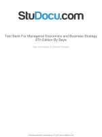
Professors Dufwenberg and Gneezy provide experimental evidence that corroborates this finding. These authors

conducted a sequence of experiments with subjects who
competed in a homogeneous product pricing game in
which marginal cost was $2 and the monopoly (collusive)
price was $100. In the experiments, sellers offering the lowest price “win” and earned real cash. As the accompanying
figure shows, theory predicts that a monopolist would price
at $100 and that prices would fall to $2 in markets with
two, three, or four sellers. In reality, the average market
price (the winning price) was about $27 when there were
only two sellers, and declined to about $9 in sessions with
three or four sellers. In practice, prices (and profits) rapidly
decline as the number of sellers increases—but not nearly
as sharply as predicted by theory.
SOURCES: Martin Dufwenberg and Uri Gneezy, “Price Competition and
Market Concentration: An Experimental Study,” International Journal
of Industrial Organization 18 (2000), pp. 7–22; Michael R. Baye, John
Morgan, and Patrick Scholten, “Price Dispersion in the Small and in the
Large: Evidence from an Internet Price Comparison Site,” Journal of
Industrial Economics 52 (2004), pp. 463–96.

$100

Market Price

$80
$60
$40
$20
$0

Predicted

Nash
Equilibrium
Price
1

Actual Price

3
2
Number of Sellers

4

To explain more precisely the preceding assertions, consider a Bertrand duopoly. Because
consumers have perfect information, and zero transaction costs, and because the products are
identical, all consumers will purchase from the firm charging the lowest price. For concreteness,
suppose firm 1 charges the monopoly price. By slightly undercutting this price, firm 2 would


www.downloadslide.net
290

CHAPTER  9  Basic Oligopoly Models

capture the entire market and make positive profits, while firm 1 would sell nothing. Therefore,
firm 1 would retaliate by undercutting firm 2’s lower price, thus recapturing the entire market.
When would this “price war” end? When each firm charged a price that equaled marginal
cost: P1 = P2 = MC. Given the price of the other firm, neither firm would choose to lower
its price, for then its price would be below marginal cost and it would make a loss. Also, no
firm would want to raise its price, for then it would sell nothing. In short, Bertrand oligopoly

and homogeneous products lead to a situation where each firm charges marginal cost and economic profits are zero. Since P = MC, homogeneous-product Bertrand oligopoly results in a
socially efficient level of output. Indeed, total market output corresponds to that in a perfectly
competitive industry, and there is no deadweight loss.
Chapters 10 and 11 provide strategies that managers can use to mitigate the “Bertrand
trap”—the cut-throat competition that ensues in homogeneous-product Bertrand oligopoly.
As we will see, the key is to either raise switching costs or eliminate the perception that the
firms’ products are identical. The product differentiation induced by these strategies permits
firms to price above marginal cost without losing customers to rivals. The appendix to this
chapter illustrates that, under differentiated-product price competition, reaction functions are
upward sloping and equilibrium occurs at a point where prices exceed marginal cost. This
explains, in part, why firms such as Kellogg’s and General Mills spend millions of dollars on
advertisements designed to persuade consumers that their competing brands of corn flakes
are not identical. If consumers did not view the brands as differentiated products, these two
makers of breakfast cereal would have to price at marginal cost.

COMPARING OLIGOPOLY MODELS
To see further how each form of oligopoly affects firms, it is useful to compare the models
covered in this chapter in terms of individual firm outputs, prices in the market, and profits per
firm. To accomplish this, we will use the same market demand and cost conditions for each firm
when examining results for each model. The inverse market demand function we will use is
​
​P = 1,000 − ​(​Q1​  ​+ ​Q2​  ​)​​
The cost function of each firm is identical and given by
​
​Ci​ ​(​Qi​ ​)​= 4​Qi​ ​​
so the marginal cost of each firm is 4. We will now see how outputs, prices, and profits vary
according to the type of oligopolistic interdependence that exists in the market.

Cournot
We will first examine Cournot equilibrium. The profit function for the individual Cournot

firm given the preceding inverse demand and cost functions is
​
​π​ i​= ​[​1,000 − ​(​Q1​  ​+ ​Q2​  ​)​]​Qi​ ​− 4​Qi​ ​​
The reaction functions of the Cournot oligopolists are
1
​Q1​  ​= ​r​ 1​(​Q2​  ​)​= 498 − __
​   ​ Q​2  ​
2
​
  
​
​​
1
​Q2​  ​= ​r​ 2(​ ​Q1​  )​ ​= 498 − __
​   ​ Q​1  ​
2


www.downloadslide.net


Managerial Economics and Business Strategy

Solving these two reaction functions for Q1 and Q2 yields the Cournot equilibrium outputs,
which are Q1 = Q2 = 332. Total output in the market thus is 664, which leads to a price of $336.
Plugging these values into the profit function reveals that each firm earns profits of $110,224.

Stackelberg
With these demand and cost functions, the output of the Stackelberg leader is
a + ​c​ 2​− 2​c​ 1​ ____________

1,000 + 4 − 2​(​4​)​
​
​Q1​  ​= _________
​ 
 
 
​ 
= ​   
 
​ 
= 498​
2b
2
The follower takes this level of output as given and produces according to its reaction function:
a − ​c​ 2​ __
1
1,000 − 4 __
1
​
​Q2​  ​= ​r​ 2​(​Q1​  ​) = _____
​ 
   
​ − ​   ​ Q​1  ​= ________
​ 
   
​ 
− ​   ​ (498) = 249​
2b
2
2

2
Total output in the market thus is 747 units. Given the inverse demand function, this output
yields a price of $253. Total market output is higher in a Stackelberg oligopoly than in a
Cournot oligopoly. This leads to a lower price in the Stackelberg oligopoly than in the Cournot
oligopoly. The profits for the leader are $124,002, while the follower earns only $62,001 in
profits. The leader does better in a Stackelberg oligopoly than in a Cournot oligopoly due to
its first-mover advantage. However, the follower earns lower profits in a Stackelberg oligopoly than in a Cournot oligopoly.

Bertrand
The Bertrand equilibrium is simple to calculate. Recall that firms that engage in Bertrand
competition end up setting price equal to marginal cost. Therefore, with the given inverse
demand and cost functions, price equals marginal cost ($4) and profits are zero for each firm.
Total market output is 996 units. Given symmetric firms, each firm gets half of the market.

Collusion
Finally, we will determine the collusive outcome, which results when the firms choose output
to maximize total industry profits. When firms collude, total industry output is the monopoly
level, based on the market inverse demand curve. Since the market inverse demand curve is
​
P = 1,000 − Q​
the associated marginal revenue is
​MR = 1,000 − 2Q​
Notice that this marginal revenue function assumes the firms act as a single profit-maximizing firm, which is what collusion is all about. Setting marginal revenue equal to marginal cost
(which is $4) yields
​
1,000 − 2Q = 4​
or Q = 498. Thus, total industry output under collusion is 498 units, with each firm producing
half. The price under collusion is
​
P = 1,000 − 498 = $502​

Each firm earns profits of $124,002.

291


www.downloadslide.net
292

CHAPTER  9  Basic Oligopoly Models

INSIDE BUSINESS 9–4

Using a Spreadsheet to Calculate Cournot, Stackelberg,
and Collusive Outcomes
Available at www.mhhe.com/baye9e, there are  three files
named CournotSolver.xls, StackelbergSolver.xls, and Collusion
Solver.xls. With a few clicks of a mouse, you can use these
files to calculate the profit-maximizing price and quantity
and the maximum profits for the following oligopoly
situations.
COURNOT DUOPOLY
In a Cournot duopoly, each firm believes the other will hold
its output constant as it changes its own output. Therefore,
the profit-maximizing output level for firm 1 depends on
firm 2’s output. Each firm will adjust its profit-maximizing
output level until the point where the two firms’ reaction
functions are equal. This point corresponds to the Cournot
equilibrium. At the Cournot equilibrium, neither firm has an
incentive to change its output, given the output of the other
firm. Step-by-step instructions for computing the Cournot

equilibrium outputs, price, and profits are included in the
file named CournotSolver.xls.

STACKELBERG DUOPOLY
The Stackelberg duopoly model assumes that one firm is
the leader while the other is a follower. The leader has a
first-mover advantage and selects its profit-maximizing output level, knowing that the follower will move second and
thus react to this decision according to a Cournot reaction
function. Given the leader’s output decision, the follower
takes the leader’s output as given and chooses its profit-maximizing level of output. Step-by-step instructions for
computing the Stackelberg equilibrium outputs, price, and
profits are included in the file named StackelbergSolver.xls.
COLLUSIVE DUOPOLY
(THE MONOPOLY SOLUTION)
Under collusion, duopolists produce a total output that corresponds to the monopoly output. In a symmetric situation,
the two firms share the market equally, each producing
one-half of the monopoly output. Step-by-step instructions
for computing the collusive (monopoly) output, price, and
profits are included in the file named CollusionSolver.xls.

Comparison of the outcomes in these different oligopoly situations reveals the following:
The highest market output is produced in a Bertrand oligopoly, followed by Stackelberg, then
Cournot, and finally collusion. Profits are highest for the Stackelberg leader and the colluding
firms, followed by Cournot, then the Stackelberg follower. The Bertrand oligopolists earn the
lowest level of profits. If you become a manager in an oligopolistic market, it is important to
recognize that your optimal decisions and profits will vary depending on the type of oligopolistic interaction that exists in the market.

CONTESTABLE MARKETS
contestable market
A market in which (1) all

firms have access to
the same technology;
(2) consumers respond
quickly to price changes;
(3) existing firms cannot
respond quickly to entry
by lowering their prices;
and (4) there are no
sunk costs.

Thus far, we have emphasized strategic interaction among existing firms in an oligopoly.
Strategic interaction can also exist between existing firms and potential entrants into a market.
To illustrate the importance of this interaction and its similarity to Bertrand oligopoly, let us
suppose a market is served by a single firm, but there is another firm (a potential entrant) free
to enter the market whenever it chooses.
Before we continue our analysis, let us make more precise what we mean by free entry.
What we have in mind here is what economists refer to as a contestable market. A market is
contestable if



1. All producers have access to the same technology.
2. Consumers respond quickly to price changes.


www.downloadslide.net

293

Managerial Economics and Business Strategy

3. Existing firms cannot respond quickly to entry by lowering price.
4. There are no sunk costs.

If these four conditions hold, incumbent firms (existing firms in the market) have no market
power over consumers. That is, the equilibrium price corresponds to marginal cost, and firms
earn zero economic profits. This is true even if there is only one existing firm in the market.
The reason for this result follows. If existing firms charged a price in excess of what they
required to cover costs, a new firm could immediately enter the market with the same technology and charge a price slightly below the existing firms’ prices. Since the incumbents cannot
quickly respond by lowering their prices, the entrant would get all the incumbents’ customers
by charging the lower price. Because the incumbents know this, they have no alternative but
to charge a low price equal to the cost of production to keep out the entrant. Thus, if a market
is perfectly contestable, incumbents are disciplined by the threat of entry by new firms.
An important condition for a contestable market is the absence of sunk costs. In this context, sunk costs are defined as costs a new entrant must bear that cannot be recouped upon
exiting the market. For example, if an entrant pays $100,000 for a truck to enter the market
for moving services, but receives $80,000 for the truck upon exiting the market, $20,000
represents the sunk cost of entering the market. Similarly, if a firm pays a nonrefundable
fee of $20,000 for the nontransferable right to lease a truck for a year to enter the market,
this reflects a sunk cost associated with entry. Or if a small firm must incur a loss of $2,000
per month for six months while waiting for customers to “switch” to that company, it incurs
$12,000 of sunk costs.
Sunk costs are important for the following reason: Suppose incumbent firms are charging
high prices, and a new entrant calculates that it could earn $70,000 by entering the market and
charging a lower price than the existing firms. This calculation is, of course, conditional upon
the existing firms continuing to charge their present prices. Suppose that to enter, the firm
must pay sunk costs of $20,000. If it enters the market and the incumbent firms keep charging

the high price, entry is profitable; indeed, the firm will make $70,000. However, if the incumbents do not continue charging the high price but instead lower their prices, the entrant can
be left with no customers. The incumbents cannot lower their prices quickly, so the entrant
may earn some profits early on; however, it likely will not earn enough profit to offset its sunk
costs before the incumbents lower their prices. In this instance, the entrant would need to
earn enough profit immediately after entering to cover its sunk cost of $20,000. In short, if a
potential entrant must pay sunk costs to enter a market and has reason to believe incumbents
will respond to entry by lowering their prices, it may find it unprofitable to enter even though
prices are high. The end result is that with sunk costs, incumbents may not be disciplined by
potential entry, and higher prices may prevail. Chapters 10 and 13 provide more detailed coverage of strategic interactions between incumbents and potential entrants.

ANSWERING THE headLINE
Although the price of crude oil fell, in a few areas there were no declines in the price of
gasoline. The headline asks whether this is evidence of collusion by gasoline stations in
those areas. To answer this question, notice that oil is an input in producing gasoline.
A reduction in the price of oil leads to a reduction in the marginal cost of producing
gasoline—say, from MC0 to MC1. If gasoline stations were colluding, a reduction in marginal cost would lead the firms to lower the price of gasoline. To see this, recall that under
collusion, both the industry output and the price are set at the monopoly level and price.

sunk cost
A cost that is forever lost
after it has been paid.


www.downloadslide.net
294

Figure 9–12
Reduction in Marginal
Cost Lowers the
Collusive Price

CHAPTER  9  Basic Oligopoly Models

Price
MC0
Due to decrease
in price of oil

P*
P **

MC1

D

0

Quantity of
Gasoline

Q * Q **

MR

Thus, if firms were colluding when marginal cost was MC0, the output that would maximize collusive profits would occur where MR = MC0 in Figure 9–12. Thus, Q* and P* in
Figure 9–12 denote the collusive output and price when marginal cost is MC0. A reduction in the marginal cost of producing gasoline would shift down the marginal cost curve
to MC1, leading to a greater collusive output (Q**) and a lower price (P**). Thus, collusion
cannot explain why some gasoline firms failed to lower their prices. Had these firms
been colluding, they would have found it profitable to lower gasoline prices when the
price of oil fell.

Since collusion is not the reason gasoline prices in some areas did not fall when
the marginal cost of gasoline declined, one may wonder what could explain the pricing
behavior in these markets. One explanation is that these gasoline producers are Sweezy
oligopolists. The Sweezy oligopolist operates on the assumption that if she raises her
price, her competitors will ignore the change. However, if she lowers her price, all will
follow suit and lower their prices. Figure 9–13 reveals that Sweezy oligopolists will not
decrease gasoline prices when marginal cost falls from MC0 to MC1. They know they cannot increase their profits or market share by lowering their price because all of their competitors will lower prices if they do.

Figure 9–13
Price Rigidity in Sweezy
Oligopoly

Price

MC0

Due to decrease
MC1 in price of oil

P*

D
0

Q*

MR

Quantity of
Gasoline