Ebook Macroeconomics - A european perspective: Part 2

www.downloadslide.com

Chapter

13

TECHNOLOGICAL PROGRESS
AND GROWTH
Our conclusion in Chapter 12 that capital accumulation cannot by itself sustain growth has a
straightforward implication: sustained growth requires technological progress. This chapter
looks at the role of technological progress in growth:
●

Section 13.1 looks at the respective role of technological progress and capital accumulation
in growth. It shows how, in steady state, the rate of growth of output per person is simply
equal to the rate of technological progress. This does not mean, however, that the saving rate
is irrelevant. The saving rate affects the level of output per person – but not its rate of growth.

●

Section 13.2 turns to the determinants of technological progress, focusing in particular on the
role of research and development (R&D).

●

Section 13.3 returns to the facts of growth presented in Chapter 11 and interprets them in
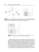
the light of what we have learned in this and the previous chapter.


www.downloadslide.com
CHAPTER 13 TECHNOLOGICAL PROGRESS AND GROWTH

269

13.1 TECHNOLOGICAL PROGRESS AND THE RATE
OF GROWTH
In an economy in which there is both capital accumulation and technological progress,
at what rate will output grow? To answer this question, we need to extend the model
developed in Chapter 12 to allow for technological progress. To introduce technological
progress into the picture, we must first revisit the aggregate production function.

Technological progress and the production function
Technological progress has many dimensions:
●
●
●
●

It can lead to larger quantities of output for given quantities of capital and labour. Think of
a new type of lubricant that allows a machine to run at a higher speed and so produce more.
It can lead to better products. Think of the steady improvement in car safety and comfort
over time.
It can lead to new products. Think of the introductions of CD players, fax machines, ➤ The average number of items carried
by a supermarket increased from 2200
mobile phones and flat-screen monitors.
It can lead to a larger variety of products. Think of the steady increase in the number of in 1950 to 45 500 in 2005 in the USA.
To get a sense of what this means,
breakfast cereals available at your local supermarket.
see Robin Williams (who plays an

These dimensions are more similar than they appear. If we think of consumers as caring not immigrant from the Soviet Union) in

the supermarket scene in the movie
about the goods themselves but about the services these goods provide, then they all have Moscow on the Hudson.
something in common: in each case, consumers receive more services. A better car provides
more safety, a new product such as a fax machine or a new service such as the Internet
provides more information services and so on. If we think of output as the set of underlying
services provided by the goods produced in the economy, we can think of technological
progress as leading to increases in output for given amounts of capital and labour. We ➤ As you saw in the Focus box ‘Real GDP,
can then think of the state of technology as a variable that tells us how much output can be technological progress and the price
produced from given amounts of capital and labour at any time. If we denote the state of of computers’ in Chapter 2, thinking
of products as providing a number of
technology by A, we can rewrite the production function as
underlying services is the method
used to construct the price index for
computers.

Y = F(K, N, A)
(+, +, +)

This is our extended production function. Output depends on both capital and labour, K and ➤ For simplicity, we ignore human capital
N, and on the state of technology, A: given capital and labour, an improvement in the state here. We return to it later in the
chapter.
of technology, A, leads to an increase in output.
It will be convenient to use a more restrictive form of the preceding equation, however,
namely
Y = F(K, AN )

[13.1]

This equation states that production depends on capital and on labour multiplied by
the state of technology. Introducing the state of technology in this way makes it easier to

think about the effect of technological progress on the relation between output, capital
and labour. Equation (13.1) implies that we can think of technological progress in two
equivalent ways:
●

●

Technological progress reduces the number of workers needed to produce a given
amount of output. Doubling A produces the same quantity of output with only half the
original number of workers, N.
Technological progress increases the output that can be produced with a given number ➤ AN is also sometimes called labour in
of workers. We can think of AN as the amount of effective labour in the economy. If efficiency units. The use of ‘efficiency’
for ‘efficiency units’ here and for
the state of technology, A, doubles, it is as if the economy had twice as many workers. ‘efficiency wages’ in Chapter 7 is
In other words, we can think of output being produced by two factors: capital, K, and a coincidence: the two notions are
unrelated.
effective labour, AN.


www.downloadslide.com

270

THE CORE THE LONG RUN

What restrictions should we impose on the extended production function (13.1)? We can
build directly here on our discussion in Chapter 11.
Again, it is reasonable to assume constant returns to scale: for a given state of technology,
A, doubling both the amount of capital, K, and the amount of labour, N, is likely to lead to
a doubling of output:

2Y = F(2K, 2AN )
More generally, for any number x,
xY = F(xK, xAN )

Per worker: divided by the number
of workers, N. Per effective worker:
divided by the number of effective
workers, AN – the number of workers,
N, times the state of technology, A.
Suppose that F has the ‘double square
root’ form:
Y 5 F(K, AN ) 5 K AN
Then
Y
K AN
K
5
5
AN
AN
AN
So the function f is simply the square
root function:
F (K /AN ) 5

K
AN

It is also reasonable to assume decreasing returns to each of the two factors – capital and
effective labour. Given effective labour, an increase in capital is likely to increase output,

but at a decreasing rate. Symmetrically, given capital, an increase in effective labour is
likely to increase output, but at a decreasing rate.
➤
It was convenient in Chapter 11 to think in terms of output per worker and capital
per worker. That was because the steady state of the economy was a state where output
per worker and capital per worker were constant. It is convenient here to look at output per
effective worker and capital per effective worker. The reason is the same: as we shall soon see,
in steady state, output per effective worker and capital per effective worker are constant.
➤
To get a relation between output per effective worker and capital per effective worker,
take x = 1/AN in the preceding equation. This gives
Y
K
= FA
, 1D
C AN F
AN
Or, if we define the function f so that f(K/AN ) ≡ F(K/AN, 1):
Y
K D
=fA
C AN F
AN
In words: output per effective worker (the left side) is a function of capital per effective
worker (the expression in the function on the right side).
The relation between output per effective worker and capital per effective worker is
drawn in Figure 13.1. It looks very much the same as the relation we drew in Figure 11.2
between output per worker and capital per worker in the absence of technological progress.
There, increases in K/N led to increases in Y/N, but at a decreasing rate. Here, increases in
K/AN lead to increases in Y/AN, but at a decreasing rate.

Interactions between output and capital
We now have the elements we need to think about the determinants of growth. Our analysis will parallel the analysis of Chapter 12. There we looked at the dynamics of output per

Figure 13.1
Output per effective
worker versus capital per
effective worker
Because of decreasing returns to
capital, increases in capital per
effective worker lead to smaller
and smaller increases in output per
effective worker.


www.downloadslide.com
CHAPTER 13 TECHNOLOGICAL PROGRESS AND GROWTH

271

Figure 13.2
The dynamics of capital
per effective worker and
output per effective worker
Capital per effective worker and output
per effective worker converge to
constant values in the long run.

worker and capital per worker. Here we look at the dynamics of output per effective worker ➤ The simple key to understanding the
results in this section is that the results

and capital per effective worker.
we derived for output per worker in
In Chapter 12, we characterised the dynamics of output and capital per worker using
Chapter 12 still hold in this chapter, but
Figure 12.2. In that figure, we drew three relations:
now for output per effective worker.
●
●
●

The relation between output per worker and capital per worker.
The relation between investment per worker and capital per worker.
The relation between depreciation per worker – equivalently, the investment per worker
needed to maintain a constant level of capital per worker – and capital per worker.

The dynamics of capital per worker and, by implication, output per worker were
determined by the relation between investment per worker and depreciation per worker.
Depending on whether investment per worker was greater or smaller than depreciation per
worker, capital per worker increased or decreased over time, as did output per worker.
We shall follow the same approach in building Figure 13.2. The difference is that we
focus on output, capital and investment per effective worker rather than per worker:
●

●

The relation between output per effective worker and capital per effective worker was
derived in Figure 13.1. This relation is repeated in Figure 13.2: Output per effective
worker increases with capital per effective worker, but at a decreasing rate.
Under the same assumptions as in Chapter 12 – that investment is equal to private
saving, and the private saving rate is constant – investment is given by

I = s = sY
Divide both sides by the number of effective workers, AN, to get
I
Y
=s
AN
AN
Replacing output per effective worker, Y/AN, by its expression from equation (13.2)
gives
I
KD
= sf A
C AN F
AN
The relation between investment per effective worker and capital per effective worker
is drawn in Figure 13.2. It is equal to the upper curve – the relation between output
per effective worker and capital per effective worker – multiplied by the saving rate, s.
This gives us the lower curve.

For example, in Chapter 12, we saw
that output per worker was constant in
steady state. In this chapter, we shall
see that output per effective worker is
constant in steady state. And so on.


www.downloadslide.com

272

THE CORE THE LONG RUN
●

In Chapter 12, we assumed gA 5 0 and ➤
gA 5 0. Our focus in this chapter is
on the implications of technological
progress, gA 0 0. But once we allow for
technological progress, introducing
population growth, gN 0 0, is straightforward. Thus, we allow for both gA 0 0
and gN 0 0.
The growth rate of the product of two ➤
variables is the sum of the growth rates
of the two variables. See Proposition 7
in Appendix 1 at the end of the book.

Finally, we need to ask what level of investment per effective worker is needed to maintain a given level of capital per effective worker.
In Chapter 12, for capital to be constant, investment had to be equal to the depreciation of the existing capital stock. Here, the answer is slightly more complicated: now that
we allow for technological progress (so A increases over time), the number of effective
workers, AN, increases over time. Thus, maintaining the same ratio of capital to effective
workers, K/AN, requires an increase in the capital stock, K, proportional to the increase
in the number of effective workers, AN. Let’s look at this condition more closely.
Let δ be the depreciation rate of capital. Let the rate of technological progress be equal
to gA. Let the rate of population growth be equal to gN. If we assume that the ratio of
employment to the total population remains constant, the number of workers, N, also
grows at annual rate gN. Together, these assumptions imply that the growth rate of
effective labour, AN, equals gA + gN. For example, if the number of workers is growing at
1% per year and the rate of technological progress is 2% per year, then the growth rate
of effective labour is equal to 3% per year.
These assumptions imply that the level of investment needed to maintain a given level
of capital per effective worker is therefore given by

I = δ K + ( gA + gN)K
or, equivalently,
I = (δ + gA + gN)K

[13.3]

An amount, δK, is needed just to keep the capital stock constant. If the depreciation
rate is 10%, then investment must be equal to 10% of the capital stock just to maintain
the same level of capital. And an additional amount, ( gA + gN)K, is needed to ensure that
the capital stock increases at the same rate as effective labour. If effective labour
increases at 3% per year, for example, then capital must increase by 3% per year to maintain the same level of capital per effective worker. Putting δK and ( gA + gN) together in
this example: if the depreciation rate is 10% and the growth rate of effective labour is
3%, then investment must equal 13% of the capital stock to maintain a constant level of
capital per effective worker.
To obtain more precisely the amount of investment per unit of effective worker needed
to keep a constant level of capital per unit of effective worker, we need to repeat the steps
taken in Section 12.1, where we derived the dynamics of capital per worker over time. Here
we derive in a similar way the dynamics of capital per unit of effective worker over time.
The dynamics of capital per unit of effective worker can be expressed as:
G
Kt+1
K
K J A t Nt
= H (1 − δ ) t + sf A t D K
C
A t+1 Nt+1 I
A t Nt
A t Nt F L A t+1 Nt+1

[13.4]

In words: capital per unit of effective worker at the beginning of year t + 1 is equal to
capital per unit of effective worker at the beginning of year t, taking into account the depreciation rate, plus investment per unit of effective worker in year t, which is equal to the
savings rate multiplied by output per unit of effective labour in year t.
If we subtract K t /A t Nt from both sides of the equation and rearrange the terms, we can
rewrite the previous equation as:
K t+1
K
K
1
1 D
K
1
1 D
K
+ sf A t D A
− t
− t = (1 − δ ) t A
C A t Nt F C 1 + g A 1 + g N F A t Nt
A t+1 Nt+1 A t Nt
A t Nt C 1 + g A 1 + g N F
If we assume, to keep things simple, that gA gN ≅ 0 and (1 + gA )(1 + gN ) ≅ 1, the previous
expression becomes:
K t+1
Kt
K
K
−
= sf A t D − (δ + gA + gN) t
C

F
A t+1 Nt+1 A t Nt
A t Nt
A t Nt

[13.5]


www.downloadslide.com
CHAPTER 13 TECHNOLOGICAL PROGRESS AND GROWTH

273

In words: the change in the stock of capital per unit of effective worker – given by the
difference between the two terms on the left side – is equal to saving per unit of effective worker – given by the first term on the right – minus depreciation per unit of effective
worker – given by the second term on the right.
To find the steady-state value of capital per unit of effective worker, let us set the left side
of the previous equation to zero to get:
K
K
sf A t D = (δ + gA + gN) t
C A t Nt F
A t Nt

[13.6]

The steady-state value of capital per unit of effective labour is such that the amount of
saving (the left side) is exactly enough to cover the depreciation of the existing capital stock
(the right side).
The level of investment per effective worker needed to maintain a given level of capital

per effective worker is represented by the upward-sloping line ‘Required investment’ in
Figure 13.2. The slope of the line equals (δ gA + gN ).

Dynamics of capital and output
We can now give a graphical description of the dynamics of capital per effective worker and
output per effective worker.
Consider a given level of capital per effective worker, say (K/AN)0 in Figure 13.2. At that
level, output per effective worker equals the vertical distance AB. Investment per effective
worker is equal to AC. The amount of investment required to maintain that level of capital
per effective worker is equal to AD. Because actual investment exceeds the investment level
required to maintain the existing level of capital per effective worker, K/AN increases.
Hence, starting from (K/AN )0, the economy moves to the right, with the level of capital
per effective worker increasing over time. This goes on until investment per effective
worker is just sufficient to maintain the existing level of capital per effective worker, until
capital per effective worker equals (K/AN )*.
In the long run, capital per effective worker reaches a constant level, and so does output
per effective worker. Put another way, the steady state of this economy is such that capital
per effective worker and output per effective worker are constant and equal to (K/AN)* and
(Y/AN )*, respectively.
This implies that, in steady state, output, Y, is growing at the same rate as effective
labour, AN (so that the ratio of the two is constant). Because effective labour grows at rate
gA + gN output growth in steady state must also equal gA + gN. The same reasoning applies ➤ If Y/AN is constant, Y must grow at the
same rate as AN. So it must grow at
to capital: because capital per effective worker is constant in steady state, capital is also
rate gA 1 gN .
growing at rate gA + gN.
Stated in terms of capital or output per effective worker, these results seem rather
abstract, but it is straightforward to state them in a more intuitive way, and this gives us our
first important conclusion:
In steady state, the growth rate of output equals the rate of population growth (gN ) plus the

rate of technological progress (gA ). By implication, the growth rate of output is independent
of the saving rate.
To strengthen your intuition, let’s go back to the argument we used in Chapter 12 to
show that, in the absence of technological progress and population growth, the economy
could not sustain positive growth forever:
●

The argument went as follows: suppose the economy tried to sustain positive output
growth. Because of decreasing returns to capital, capital would have to grow faster than
output. The economy would have to devote a larger and larger proportion of output to
capital accumulation. At some point, there would be no more output to devote to capital
accumulation. Growth would come to an end.


www.downloadslide.com

274

THE CORE THE LONG RUN

Table 13.1 The characteristics of balanced growth
Rate of growth of:
1 Capital per effective worker

●

0

2 Output per effective worker

0

3 Capital per worker

gA

4 Output per worker

gA

5 Labour

gN

6 Capital

gA + g N

7 Output

gA + g N

Exactly the same logic is at work here. Effective labour grows at rate gA + gN. Suppose the
economy tried to sustain output growth in excess of gA + gN. Because of decreasing returns
to capital, capital would have to increase faster than output. The economy would have to
devote a larger and larger proportion of output to capital accumulation. At some point,
this would prove impossible. Thus the economy cannot permanently grow faster than
gA + gN.

The standard of living is given by out- ➤

We have focused on the behaviour of aggregate output. To get a sense of what happens
put per worker (or, more accurately,
not to aggregate output but rather to the standard of living over time, we must look instead
output per person), not output per
at the behaviour of output per worker (not output per effective worker). Because output
effective worker.

The growth rate of Y/N is equal to the
growth rate of Y minus the growth rate
of N (see Proposition 8 in Appendix 1 at
the end of the book). So the growth rate
of Y/N is given by (gA 2 gN ) 5 (gA 1 gN )
2 gN 1 gA .

grows at rate ( gA + gN) and the number of workers grows at rate gN, output per worker grows
at rate gA. In other words, when the economy is in steady state, output per worker grows at the
rate of technological progress.
➤
Because output, capital, and effective labour all grow at the same rate, gA + gN, in steady
state, the steady state of this economy is also called a state of balanced growth: in steady
state, output and the two inputs, capital and effective labour, grow ‘in balance’, at the same
rate. The characteristics of balanced growth will be helpful later in the chapter and are
summarised in Table 13.1.
On the balanced growth path (equivalently: in steady state, or in the long run):
●
●
●

Capital per effective worker and output per effective worker are constant; this is the result
we derived in Figure 13.2.

Equivalently, capital per worker and output per worker are growing at the rate of technological progress, gA.
Or, in terms of labour, capital and output: labour is growing at the rate of population
growth, gN; capital and output are growing at a rate equal to the sum of population
growth and the rate of technological progress gA + gN.

The effects of the saving rate
In steady state, the growth rate of output depends only on the rate of population growth and
the rate of technological progress. Changes in the saving rate do not affect the steady-state
growth rate, but changes in the saving rate do increase the steady-state level of output per
effective worker.
This result is best seen in Figure 13.3, which shows the effect of an increase in the saving
rate from s0 to s1. The increase in the saving rate shifts the investment relation up, from
s0 f(K/AN) to s1 f(K/AN ). It follows that the steady-state level of capital per effective worker
increases from (K/AN)0 to (K/AN)1, with a corresponding increase in the level of output per
effective worker from (Y/AN)0 to (Y/AN)1.
Following the increase in the saving rate, capital per effective worker and output per
effective worker increase for some time, as they converge to their new higher level. Figure 13.4 plots output against time. Output is measured on a logarithmic scale. The economy
is initially on the balanced growth path AA: output is growing at rate gA + gN – so the slope


www.downloadslide.com
CHAPTER 13 TECHNOLOGICAL PROGRESS AND GROWTH

275

Figure 13.3
The effects of an increase
in the saving rate (1)
An increase in the saving rate leads to
an increase in the steady-state levels of

output per effective worker and capital
per effective worker.

Figure 13.4
The effects of an increase
in the saving rate (2)
The increase in the saving rate leads
to higher growth until the economy
reaches its new, higher, balanced
growth path.

of AA is equal to gA + gN. After the increase in the saving rate at time t, output grows faster ➤ Figure 13.4 is the same as Figure 12.5,
which anticipated the derivation prefor some period of time. Eventually, output ends up at a higher level than it would have
sented here.
been without the increase in saving, but its growth rate returns to gA + gN. In the new steady
For a description of logarithmic scales,
state, the economy grows at the same rate, but on a higher growth path, BB. BB, which is
see Appendix 1 at the end of the book.
parallel to AA, also has a slope equal to gA + gN.
Let’s summarise: in an economy with technological progress and population growth, out- ➤ When a logarithmic scale is used, a
variable growing at a constant rate
put grows over time. In steady state, output per effective worker and capital per effective
moves along a straight line. The slope
worker are constant. Put another way, output per worker and capital per worker grow at the
of the line is equal to the rate of growth
rate of technological progress. Put yet another way, output and capital grow at the same
of the variable.
rate as effective labour and, therefore, at a rate equal to the growth rate of the number of
workers plus the rate of technological progress. When the economy is in steady state, it is
said to be on a balanced growth path.

The rate of output growth in steady state is independent of the saving rate. However,
the saving rate affects the steady-state level of output per effective worker. Increases in the
saving rate lead, for some time, to an increase in the growth rate above the steady-state
growth rate.

13.2 THE DETERMINANTS OF TECHNOLOGICAL PROGRESS
We have just seen that the growth rate of output per worker is ultimately determined by the
rate of technological progress. This leads naturally to the next question: what determines
the rate of technological progress? We now take up this question.


www.downloadslide.com

276

THE CORE THE LONG RUN

‘Technological progress’ brings to mind images of major discoveries: the invention of the
microchip, the discovery of the structure of DNA and so on. These discoveries suggest a process driven largely by scientific research and chance rather than by economic forces. But the
truth is that most technological progress in modern economies is the result of a humdrum
process: the outcome of firms’ research and development (R&D) activities. Industrial
R&D expenditures account for between 2% and 3% of GDP in each of the four major rich
countries we looked at in Chapter 11 (the USA, France, Japan and the UK). About 75% of
the roughly 1 million US scientists and researchers working in R&D are employed by firms.
US firms’ R&D spending equals more than 20% of their spending on gross investment and
more than 60% of their spending on net investment – gross investment less depreciation.
Firms spend on R&D for the same reason they buy new machines or build new plants: to
increase profits. By increasing spending on R&D, a firm increases the probability that it will
discover and develop a new product. (We use product as a generic term to denote new
goods or new techniques of production.) If a new product is successful, the firm’s profits will

increase. There is, however, an important difference between purchasing a machine and
spending more on R&D. The difference is that the outcome of R&D is fundamentally ideas.
And, unlike a machine, an idea can potentially be used by many firms at the same time.
A firm that has just acquired a new machine does not have to worry that another firm will
use that particular machine. A firm that has discovered and developed a new product can
make no such assumption.
This last point implies that the level of R&D spending depends not only on the fertility of
the research process – how spending on R&D translates into new ideas and new products –
but also on the appropriability of research results – the extent to which firms benefit from
the results of their own R&D. Let’s look at each aspect in turn.

The fertility of the research process

In Chapter 12, we looked at the role
of human capital as an input in production: more educated people can use
more complex machines, or handle
more complex tasks. Here, we see
a second role of human capital: better
researchers and scientists and, by
implication, a higher rate of technological progress.

If research is very fertile – that is, if R&D spending leads to many new products – then, other
things being equal, firms will have strong incentives to spend on R&D; R&D spending and,
by implication, technological progress will be high. The determinants of the fertility of
research lie largely outside the realm of economics. Many factors interact here.
The fertility of research depends on the successful interaction between basic research
(the search for general principles and results) and applied research and development (the
application of these results to specific uses and the development of new products). Basic
research does not lead, by itself, to technological progress, but the success of applied
research and development depends ultimately on basic research. Much of the computer

industry’s development can be traced to a few breakthroughs, from the invention of the
transistor to the invention of the microchip. Indeed, the recent increase in productivity
growth in the USA, which we discussed in Chapter 1, is widely attributed to the diffusion
across the US economy of the breakthroughs in information technology. (This is explored
further in the Focus box ‘Information technology, the new economy and productivity
growth’.)
➤
Some countries appear to be more successful than others at basic research; other countries are more successful at applied research and development. Studies point to differences
in the education system as one of the reasons. For example, it is often argued that the
French higher education system, with its strong emphasis on abstract thinking, produces
researchers who are better at basic research than at applied research and development.
Studies also point to the importance of a ‘culture of entrepreneurship,’ in which a big part
of technological progress comes from the ability of entrepreneurs to organise the successful
development and marketing of new products – a dimension where the USA appears to be
better than most other countries.
It takes many years, and often many decades, for the full potential of major discoveries
to be realised. The usual sequence is that a major discovery leads to the exploration of
potential applications, then to the development of new products and, finally, to the adoption


www.downloadslide.com
CHAPTER 13 TECHNOLOGICAL PROGRESS AND GROWTH

277

FOCUS
Information technology, the new economy and productivity growth
Average annual productivity growth in the USA from
1996 –2006 reached 2.8% – a high number relative to the
anaemic 1.8% average achieved from 1970–1995. This

has led some to proclaim an information technology
revolution, announce the dawn of a New Economy and
forecast a long period of high productivity growth in the
future.
What should we make of these claims? Research to
date gives reasons both for optimism and for caution. It
suggests that the recent high productivity growth is
indeed linked to the development of information technologies. It also suggests that a sharp distinction must be
drawn between what is happening in the information
technology (IT) sector – the sector that produces computers, computer software and software services and
communications equipment – and the rest of the economy
– which uses this information technology:
In the IT sector, technological progress has indeed been
proceeding at an extraordinary pace.

Figure 13.5
Moore’s law: number of transistors per chip, 1970–2000
Source: Dale Jorgenson, ‘Information Technology and the US Economy ’, American Economic Review,
2001, 91(1), 1–32.

▼

●

In 1965, researcher Gordon Moore, who later founded
Intel Corporation, predicted that the number of transistors in a chip would double every 18 –24 months,
allowing for steadily more powerful computers. As
shown in Figure 13.5, this relation – now known as
Moore’s law – has held extremely well over time. The
first logic chip produced in 1971 had 2300 transistors;

the Pentium 4, released in 2000, had 42 million. (The
Intel Core 2, released in 2006, and thus not included
in the figure, has 291 million.)
Although it has proceeded at a less extreme pace,
technological progress in the rest of the IT sector has
also been very high. And the share of the IT sector in
GDP is steadily increasing, from 3% of GDP in 1980 to
7% today. This combination of high technological
progress in the IT sector and of an increasing IT share
has led to a steady increase in the economy-wide rate
of technological progress. This is one of the factors
behind the high productivity growth in the USA since
the mid-1990s.


www.downloadslide.com

278

●

THE CORE THE LONG RUN

However, in the non-IT sector – the ‘old economy,’
which still accounts for more than 90% of the US
economy – there is little evidence of a parallel technological revolution:
On the one hand, the steady decrease in the price of
IT equipment (reflecting technological progress in the
IT sector) has led firms in the non-IT sector to increase
their stock of IT capital. This has led to an increase

in the ratio of capital per worker and an increase in
productivity growth in the non-IT sector.
Let’s go through this argument a bit more formally.
Go back to equation (13.2), which shows the relation
of output per effective worker to the ratio of capital per
effective worker:
Y/AN = f(K/AN)

●

Think of this equation as giving the relation between
output per effective worker and capital per effective
worker in the non-IT sector. The evidence is that the
decrease in the price of IT capital has led firms to
increase their stock of IT capital and, by implication,
their overall capital stock. In other words, K /AN has
increased in the non-IT sector, leading to an increase
in Y/AN.
On the other hand, the IT revolution does not appear to
have had a major direct effect on the pace of technological progress in the non-IT sector. You have surely
heard claims that the information technology revolution was forcing firms to drastically reorganise, leading

to large gains in productivity. Firms may be reorganising but, so far, there is little evidence that this is leading
to large gains in productivity: measures of technological
progress show only a small rise in the rate of technological progress in the non-IT sector from the post1970 average.
In terms of the production function relation we just
discussed, there is no evidence that the technological
revolution has led to a higher rate of growth of A in the
non-IT sector.
Are there reasons to expect productivity growth to be

higher in the future than in the past 25 years? The answer
is yes: the factors we have just discussed are here to stay.
Technological progress in the IT sector is likely to remain
high, and the share of IT is likely to continue to increase.
Moreover, firms in the non-IT sector are likely to further
increase their stock of IT capital, leading to further
increases in productivity.
How high can we expect productivity growth to be
in the future? Probably not as high as it was from
1996–2006 but, according to some estimates, we can
expect it to be perhaps 0.5 percentage points higher than
its post-1970 average. This may not be the miracle some
have claimed but, if sustained, it is an increase that will
make a substantial difference to the US standard of living
in the future.
Note: For more on these issues, read ‘Information Technology
and the U.S. Economy’, by Dale Jorgenson, American Economic
Review, 2001, 91(1), 1–32.

of these new products. An example with which we are all familiar is the personal computer.
Twenty years after the commercial introduction of personal computers, it often seems as if
we have just begun discovering their uses.
An age-old worry is that research will become less and less fertile – that most major discoveries have already taken place and that technological progress will now slow down. This
fear may come from thinking about mining, where higher-grade mines were exploited first,
and we have had to exploit lower- and lower-grade mines. But this is only an analogy, and
so far there is no evidence that it is correct.

The appropriability of research results
The second determinant of the level of R&D and of technological progress is the degree of
appropriability of research results. If firms cannot appropriate the profits from the development of new products, they will not engage in R&D, and technological progress will be slow.

Many factors are also at work here.
The nature of the research process itself is important. For example, if it is widely believed
that the discovery of a new product by one firm will quickly lead to the discovery of an even
better product by another firm, there may be little payoff to being first. In other words,
a highly fertile field of research may not generate high levels of R&D because no company
will find the investment worthwhile. This example is extreme but revealing.


www.downloadslide.com
CHAPTER 13 TECHNOLOGICAL PROGRESS AND GROWTH

279

Even more important is the legal protection given to new products. Without such legal
protection, profits from developing a new product are likely to be small. Except in rare cases
where the product is based on a trade secret (such as Coca-Cola), it will generally not take
long for other firms to produce the same product, eliminating any advantage the innovating
firm may have had initially. This is why countries have patent laws. A patent gives a firm
that has discovered a new product – usually a new technique or device – the right to exclude
anyone else from the production or use of the new product for some time.
How should governments design patent laws? On the one hand, protection is needed ➤ This type of dilemma is known as ‘time
to provide firms with the incentives to spend on R&D. On the other, once firms have dis- inconsistency.’ We shall see other
covered new products, it would be best for society if the knowledge embodied in those examples and discuss it at length in
Chapter 23.
new products were made available to other firms and to people without restrictions. Take,
The issues go beyond patent laws.
for example, biogenetic research. Only the prospect of large profits is leading bioengineering
To take two controversial examples:
firms to embark on expensive research projects. Once a firm has found a new product, and should Microsoft be kept in one piece
the product can save many lives, it would clearly be best to make it available at cost to all or broken up to stimulate R&D? Should

potential users. But if such a policy was systematically followed, it would eliminate incen- the government impose caps on the
tives for firms to do research in the first place. So, patent law must strike a difficult balance. prices of AIDS drugs?
Too little protection will lead to little R&D. Too much protection will make it difficult for
new R&D to build on the results of past R&D and may also lead to little R&D. (The difficulty
of designing good patent or copyright laws is illustrated in the cartoon about cloning.)

Source: © Chappatte-www.globecartoon.com.

Countries that are less technologically advanced than others often have poorer patent
protection. China, for example, is a country with poor enforcement of patent rights. Our
discussion helps explain why. These countries are typically users rather than producers of
new technologies. Much of their improvement in productivity comes not from inventions
within the country but from the adaptation of foreign technologies. In this case, the costs of
weak patent protection are small because there would be few domestic inventions anyway.
But the benefits of low patent protection are clear: domestic firms can use and adapt
foreign technology without having to pay royalties to the foreign firms that developed the
technology – which is good for the country.


www.downloadslide.com

280

THE CORE THE LONG RUN

13.3 THE FACTS OF GROWTH REVISITED
We can now use the theory we have developed in this chapter and Chapter 12 to interpret
some of the facts we saw in Chapter 11.

Capital accumulation versus technological progress in rich

countries since 1950
Suppose we observe an economy with a high growth rate of output per worker over some
period of time. Our theory implies that this fast growth may come from two sources:
●
●

In the USA, for example, the ratio of
employment to population increased
from 38% in 1950 to 51% in 2006.
This represents an increase of 0.18%
per year. Thus, in the USA, output per
person has increased 0.18% more per
year than output per worker – a small
difference, relative to the numbers in
the table.

What would have happened to the
growth rate of output per worker if
these countries had had the same rate
of technological progress but no capital
accumulation during the period?

It may reflect a high rate of technological progress under balanced growth.
It may reflect instead the adjustment of capital per effective worker, K/AN, to a higher
level. As we saw in Figure 13.5, such an adjustment leads to a period of higher growth,
even if the rate of technological progress has not increased.

Can we tell how much of the growth comes from one source and how much comes from
the other? Yes. If high growth reflects high balanced growth, output per worker should be
growing at a rate equal to the rate of technological progress (see Table 13.1, row 4). If high

growth reflects instead the adjustment to a higher level of capital per effective worker, this
adjustment should be reflected in a growth rate of output per worker that exceeds the rate
of technological progress.
Let’s apply this approach to interpret the facts about growth in rich countries we saw in
Table 11.1. This is done in Table 13.2, which gives, in column 1, the average rate of growth
➤ of output per worker, gY − gN, and, in column 2, the average rate of technological progress,
gA, since 1950, for each of the six countries – France, Ireland, Japan, Sweden, the UK and
the USA – we looked at in Table 11.1. (Note one difference between Tables 11.1 and 13.2:
as suggested by the theory, Table 13.2 looks at the growth rate of output per worker, while
Table 11.1, which focuses on the standard of living, looks at the growth rate of output per
person. The differences are small.) The rate of technological progress, gA, is constructed
using a method introduced by Robert Solow; the method and the details of construction are
given in the Focus box ‘Constructing a measure of technological progress’.
The table leads to two conclusions. First, growth since 1950 has been a result of rapid
technological progress, not unusually high capital accumulation. This conclusion follows
from the fact that, in all four countries, the growth rate of output per worker (column 1) has
been roughly equal to the rate of technological progress (column 2). This is what we would
expect when countries are growing along their balanced growth path.
➤
Note what this conclusion does not say: it does not say that capital accumulation was
irrelevant. Capital accumulation was such as to allow these countries to maintain a roughly
constant ratio of output to capital and achieve balanced growth. What it says is that, over
Table 13.2 Average annual rates of growth of output per worker and technological
progress in six rich countries since 1950

France
Ireland
Japan
Sweden
UK

USA
Average

Rate of growth of output
per worker (%) 1950–2004

Rate of technological
progress (%) 1950–2004

3.02
–
4.02
–
2.04
1.08

3.01
–
3.08
–
2.06
2.00

Note: ‘Average’ is a simple average of the growth rates in each column.
Sources: 1950–1970: Angus Maddison, Dynamic Forces in Capitalist Development, Oxford University Press, New York,
1991; 1970–2004: OECD Economic Outlook database.


www.downloadslide.com
CHAPTER 13 TECHNOLOGICAL PROGRESS AND GROWTH

281

the period, growth did not come from an unusual increase in capital accumulation, it came
from an increase in the ratio of capital to output.
Second, convergence of output per worker across countries has come from higher
technological progress, rather than from faster capital accumulation, in the countries that
started behind. This conclusion follows from the ranking of the rates of technological
progress across the four countries in the second column, with Japan at the top and the USA
at the bottom.
This is an important conclusion. One can think, in general, of two sources of convergence ➤ While the table looks at only four countries, a similar conclusion holds when
between countries. First, poorer countries are poorer because they have less capital to start
one looks at the set of all OECD counwith. Over time, they accumulate capital faster than the others, generating convergence.
tries. Convergence is mainly due to the
Second, poorer countries are poorer because they are less technologically advanced than
fact that countries that were behind in
the others. Over time, they become more sophisticated, either by importing technology
1950 have had higher rates of technofrom advanced countries or developing their own. As technological levels converge, so does
logical progress since then.
output per worker. The conclusion we can draw from Table 13.2 is that, in the case of rich
countries, the more important source of convergence in this case is clearly the second one.

FOCUS
Constructing a measure of technological progress

∆Y =

W
∆N
P

Divide both sides of the equation by Y, divide and multiply
the right side by N and reorganise:
∆Y WN ∆N
=
Y
PY N
Note that the first term on the right, WN/PY, is equal to
the share of labour in output – the total wage bill in
pounds divided by the value of output in pounds. Denote
this share by α. Note that ∆Y/ Y is the rate of growth of
output and denote it by gY. Note similarly that ∆N/N is the

rate of change of the labour input and denote it by gN.
Then the previous relation can be written as
g Y = α gN
More generally, this reasoning implies that the part of
output growth attributable to growth of the labour input
is equal to α times gN. If, for example, employment grows
by 2%, and the share of labour is 0.7, then the output
growth due to the growth in employment is equal to 1.4%
(0.7 × 2%).
Similarly, we can compute the part of output growth
attributable to growth of the capital stock. Because there
are only two factors of production, labour and capital, and
because the share of labour is equal to α, the share of
capital in income must be equal to 1 − α. If the growth rate
of capital is equal to gK, then the part of output growth
attributable to growth of capital is equal to 1 − α times gK.
If, for example, capital grows by 5%, and the share of

capital is 0.3, then the output growth due to the growth
of the capital stock is equal to 1.5% (0.3 × 5%).
Putting the contributions of labour and capital
together, the growth in output attributable to growth in
both labour and capital is equal to α gN + (1 − α)gK.
We can then measure the effects of technological
progress by computing what Solow called the residual, the
excess of actual growth of output, gY, over the growth
attributable to growth of labour and the growth of capital,
α gN + (1 − α)gK :
Residual ≡ gY − [α gN + (1 − α)gK]

▼

In 1957, Robert Solow devised a way of constructing an
estimate of technological progress. The method, which is
still in use today, relies on one important assumption: that
each factor of production is paid its marginal product.
Under this assumption, it is easy to compute the contribution of an increase in any factor of production to the
increase in output. For example, if a worker is paid a30 000
a year, the assumption implies that her contribution to
output is equal to a30 000. Now suppose that this worker
increases the number of hours she works by 10%. The
increase in output coming from the increase in her hours
will therefore be equal to a30 000 × 10%, or a3000.
Let us write this more formally. Denote output by Y,
labour by N and the real wage by W/P. Then, we just
established the change in output is equal to the real wage
multiplied by the change in labour:

www.downloadslide.com

282

THE CORE THE LONG RUN

This measure is called the Solow residual. It is easy
to compute: all we need to know to compute it are the
growth rate of output, gY, the growth rate of labour, gN,
and the growth rate of capital, gK, together with the shares
of labour, α and capital, 1 − α.
To continue with our previous numeric examples,
suppose employment grows by 2%, the capital stock
grows by 5% and the share of labour is 0.7 (and so the
share of capital is 0.3). Then the part of output growth
attributable to growth of labour and growth of capital
is equal to 2.9% (0.7 × 2% + 0.3 × 5%). If output growth
is equal, for example, to 4%, then the Solow residual is
equal to 1.1% (4% − 2.9%).
The Solow residual is sometimes called the rate of
growth of total factor productivity (or the rate of TFP
growth, for short). The use of total factor productivity is to
distinguish it from the rate of growth of labour productivity, which is defined as gY − gN, the rate of output growth
minus the rate of labour growth.
The Solow residual is related to the rate of technological progress in a simple way. The residual is equal
to the share of labour times the rate of technological
progress:
Residual = αgA
We shall not derive this result here. But the intuition

for this relation comes from the fact that what matters in
the production function Y = F(K, AN) [equation (13.1)] is
the product of the state of technology and labour, AN.

We saw that to get the contribution of labour growth to
output growth, we must multiply the growth rate of
labour by its share. Because N and A enter the production
function in the same way, it is clear that to get the contribution of technological progress to output growth, we
must also multiply it by the share of labour.
If the Solow residual is equal to 0, so is technological
progress. To construct an estimate of gA, we must construct the Solow residual and then divide it by the share of
labour. This is how the estimates of gA presented in the
text are constructed.
In the numerical example we saw earlier, the Solow
residual is equal to 1.1%, and the share of labour is equal
to 0.7. So the rate of technological progress is equal to
1.6% (1.1%/0.7).
Keep straight the definitions of productivity growth
you have seen in this chapter:
●
●

Labour productivity growth (equivalently: the rate of
growth of output per worker), gY − gN.
The rate of technological progress, gA.

In steady state, labour productivity growth, gY − gN,
equals the rate of technological progress, gA. Outside
steady state, they need not be equal: an increase in the
ratio of capital per effective worker, due, for example, to

an increase in the saving rate, will cause gY − gN to be
higher than gA for some time.
Source: Robert Solow, ‘Technical Change and the Aggregate Production
Function’, Review of Economics and Statistics, 1957, 39(3), 312–320.

Capital accumulation versus technological progress in
China since 1980
Going beyond growth in OECD countries, one of the striking facts in Chapter 11 was the
high growth rates achieved by a number of Asian countries. This raises again the same questions we just discussed: do these high growth rates reflect fast technological progress, or do
they reflect unusually high capital accumulation?
To answer the questions, we shall focus on China because of its size and because of
the astonishingly high output growth rate, nearly 10%, it has achieved since the early
1980s. Table 13.3 gives the average rate of growth, gY, the average rate of growth of output
per worker, gY − gN, and the average rate of technological progress, gA, for the period
1983–2003. The fact that the last two numbers are nearly equal yields a very clear conclusion: growth in China since the early 1980s has been nearly balanced, and the high

Table 13.3 Average annual rate of growth of output per worker and technological
progress in China, 1983–2003
Rate of growth
of output (%)

Rate of growth of
output per worker (%)

Rate of technological
progress (%)

9.7

8.0

8.2

Source: OECD Economic Survey of China, 2005.


www.downloadslide.com
CHAPTER 13 TECHNOLOGICAL PROGRESS AND GROWTH

283

growth of output per worker reflects a high rate of technological progress, 8.2% per year
on average.
This is an important conclusion, showing the crucial role of technological progress in
explaining China’s growth. But, just as in our discussion of OECD countries, it would be
wrong to conclude that capital accumulation is irrelevant. To sustain balanced growth at
such a high growth rate, the Chinese capital stock has had to increase at the same rate as
output. This in turn has required a very high investment rate. To see what investment rate ➤ Recall, from Table 13.1: under balanced
growth, gK 5 gY 5 gA 1 gN .
was required, go back to equation (13.3) and divide both sides by output, Y, to get
1
K
= (δ + ( gA + gN))
Y
Y
Let’s plug in numbers for China for the period 1983–2003. The estimate of d, the depreciation rate of capital in China, is 5% a year. As we just saw, the average value of gA for the
period was 8.2%. The average value of gN, the rate of growth of employment, was 1.7%. The
average value of the ratio of capital to output was 2.6. This implies a ratio of investment to
output of (5% + 9.2% + 1.7%) × 2.6 = 41%. Thus, to sustain balanced growth, China has had
to invest 41% of its output, a very high investment rate in comparison to, say, the US investment rate. So capital accumulation plays an important role in explaining Chinese growth;

but it is still the case that sustained growth has come from a high rate of technological
progress.
How has China been able to achieve such technological progress? A closer look at the ➤ This ratio indeed is very close to the
data suggests two main channels. First, China has transferred labour from the countryside, ratio one gets by looking directly at
where productivity is very low, to industry and services in the cities, where productivity is investment and output in the Chinese
national income accounts.
much higher. Second, China has imported the technology of more technologically advanced
countries. It has, for example, encouraged the development of joint ventures between
Chinese firms and foreign firms. Foreign firms have come up with better technologies and,
over time, Chinese firms have learned how to use them.
This leads to a general point: the nature of technological progress is likely to be different
in more and less advanced economies. The more advanced economies, being by definition
at the technological frontier, need to develop new ideas, new processes and new products.
They need to innovate. The countries that are behind can instead improve their level of
technology by copying and adapting the new processes and products developed in the more
advanced economies. They need to imitate. The further behind a country is, the larger the
role of imitation relative to innovation. As imitation is likely to be easier than innovation,
this can explain why convergence, both within the OECD and in the case of China and other
countries, typically takes the form of technological catch-up. It raises, however, yet
another question: if imitating is so easy, why is it that so many other countries do not seem
to be able to do the same and grow? This points to the broader aspects of technology we
discussed earlier in the chapter. Technology is more than just a set of blueprints. How
efficiently the blueprints can be used and how productive an economy is depend on its
institutions, on the quality of its government and so on.

SUMMARY
●

When we think about the implications of technological
progress for growth, it is useful to think of technological

progress as increasing the amount of effective labour
available in the economy (that is, labour multiplied by
the state of technology). We can then think of output as
being produced with capital and effective labour.

●

In steady state, output per effective worker and capital per
effective worker are constant. Put another way, output per

worker and capital per worker grow at the rate of technological progress. Put yet another way, output and capital
grow at the same rate as effective labour, thus at a rate
equal to the growth rate of the number of workers plus
the rate of technological progress.
●

When the economy is in steady state, it is said to be on a
balanced growth path. Output, capital and effective labour
are all growing ‘in balance’ – that is, at the same rate.


www.downloadslide.com

284

THE CORE THE LONG RUN

●

The rate of output growth in steady state is independent

of the saving rate. However, the saving rate affects the
steady-state level of output per effective worker. And
increases in the saving rate will lead, for some time, to an
increase in the growth rate above the steady-state growth
rate.

●

Technological progress depends on both (1) the fertility
of research and development – how spending on R&D
translates into new ideas and new products – and (2) the
appropriability of the results of R&D – the extent to which
firms benefit from the results of their R&D.

●

When designing patent laws, governments must balance
their desire to protect future discoveries and provide
incentives for firms to do R&D with their desire to make
existing discoveries available to potential users without
restrictions.

●

France, Japan, the UK and the USA have experienced
roughly balanced growth since 1950: growth of output
per worker has been roughly equal to the rate of technological progress. The same is true of China. Growth in
China is roughly balanced, sustained by a high rate of
technological progress and a high investment rate.

KEY TERMS
effective labour, or labour
in efficiency units 269

appropriability of
research 276

balanced growth 274

information technology
revolution 277

research and development
(R&D) 276
fertility of research 276

New Economy 277

patent 279

technology frontier 283

Solow residual, or rate of
growth of total factor
productivity, or rate of TFP
growth 282

technological catch-up 283

Moore’s law 277

QUESTIONS AND PROBLEMS
QUICK CHECK

2. R&D and growth

1. Using the information in this chapter, label each of the
following statements true, false or uncertain. Explain briefly.

a. Why is the amount of R&D spending important for
growth? How do the appropriability and fertility of
research affect the amount of R&D spending?

a. Writing the production function in terms of capital and
effective labour implies that as the level of technology
increases by 10%, the number of workers required to
achieve the same level of output decreases by 10%.

How do each of the policy proposals listed in (b) through (e)
affect the appropriability and fertility of research, R&D spending in the long run, and output in the long run?

b. If the rate of technological progress increases, the investment rate (the ratio of investment to output) must increase
in order to keep capital per effective worker constant.

b. An international treaty that ensures that each country’s
patents are legally protected all over the world.

c. In steady state, output per effective worker grows at the
rate of population growth.

d. A decrease in funding of government-sponsored conferences between universities and corporations.

d. In steady state, output per worker grows at the rate of
technological progress.

e. The elimination of patents on breakthrough drugs, so the
drugs can be sold at low cost as soon as they are available.

e. A higher saving rate implies a higher level of capital per
effective worker in the steady state and thus a higher rate
of growth of output per effective worker.

3. Sources of technological progress: economic leaders
versus developing countries

f. Even if the potential returns from R&D spending are
identical to the potential returns from investing in a new
machine, R&D spending is much riskier for firms than
investing in new machines.
g. The fact that one cannot patent a theorem implies that
private firms will not engage in basic research.
h. Because eventually we will know everything, growth will
have to come to an end.

c. Tax credits for each euro of R&D spending.

a. Where does technological progress come from for the
economic leaders of the world?
b. Do developing countries have other alternatives to the
sources of technological progress you mentioned in

part (a)?
c. Do you see any reasons developing countries may choose
to have poor patent protection? Are there any dangers in
such a policy (for developing countries)?


www.downloadslide.com
CHAPTER 13 TECHNOLOGICAL PROGRESS AND GROWTH

6. Suppose that the economy’s production function is

DIG DEEPER
4. For each of the economic changes listed in (a) and (b),
assess the likely impact on the growth rate and the level of
output over the next five years and over the next five decades.
a. a permanent reduction in the rate of technological
progress.
b. a permanent reduction in the saving rate.
5. Measurement error, inflation and productivity
growth
Suppose that there are only two goods produced in an
economy: haircuts and banking services. Prices, quantities
and the number of workers occupied in the production of
each good for year 1 and for year 2 are given below:
Year 1
Haircut
Banking

285

Year 2

P1

Q1

W1

P2

Q2

W2

10
10

100
200

50
50

12
12

100
230

50

60

Y = K AN
that the saving rate, s, is equal to 16%, and that the rate of
depreciation, δ, is equal to 10%. Suppose further that the
number of workers grows at 2% per year and that the rate of
technological progress is 4% per year.
a. Find the steady-state values of the variables listed in (i)
through (v).
i. The capital stock per effective worker.
ii. Output per effective worker.
iii. The growth rate of output per effective worker.
iv. The growth rate of output per worker.
v. The growth rate of output.
b. Suppose that the rate of technological progress doubles
to 8% per year. Recompute the answers to part (a).
Explain.
c. Now suppose that the rate of technological progress is
still equal to 4% per year, but the number of workers now
grows at 6% per year. Re-compute the answers to (a). Are
people better off in (a) or in (c)? Explain.

a. What is nominal GDP in each year?
b. Using year 1 prices, what is real GDP in year 2? What is
the growth rate of real GDP?
c. What is the rate of inflation using the GDP deflator?
d. Using year 1 prices, what is real GDP per worker in
year 1 and year 2? What is labour productivity growth
between year 1 and year 2 for the whole economy?
Now suppose that banking services in year 2 are not the same

as banking services in year 1. Year 2 banking services include
telebanking that year 1 banking services did not include. The
technology for telebanking was available in year 1, but the
price of banking services with telebanking in year 1 was b13,
and no-one chose to purchase this package. However, in year
2, the price of banking services with telebanking was b12, and
everyone chose to have this package (i.e. in year 2 no-one
chose to have the year 1 banking services package without
telebanking). (Hint: assume that there are now two types of
banking services: those with telebanking and those without.
Rewrite the preceding table but now with three goods: haircuts
and the two types of banking services.)
e. Using year 1 prices, what is real GDP for year 2? What is
the growth rate of real GDP?
f. What is the rate of inflation using the GDP deflator?
g. What is labour productivity growth between year 1 and
year 2 for the whole economy?
h. Consider this statement: ‘If banking services are mismeasured – for example, by not taking into account
the introduction of telebanking – we will over-estimate
inflation and underestimate productivity growth.’
Discuss this statement in light of your answers to parts
(a) through (g).

7. Discuss the potential role of each of the factors listed in (a)
through (g) on the steady-state level of output per worker. In
each case, indicate whether the effect is through A, through K,
through H, or through some combination of A, K and H.
a. geographic location
b. education
c. protection of property rights

d. openness to trade
e. low tax rates
f. good public infrastructure
g. low population growth

EXPLORE FURTHER
8. Growth accounting
The Focus box ‘Constructing a measure of technological
progress’ shows how data on output, capital and labour can be
used to construct estimates of the rate of growth of technological progress. We modify that approach in this problem to
examine the growth of capital per worker. The function
Y = K 1/3(AN)2/3
gives a good description of production in rich countries. Following the same steps as in the Focus box, you can show that
(2/3)gA = gY − (2/3)gN − (1/3)gK
= (gY − gN) − (1/3)( gK − gN)
where gx denotes the growth rate of x.
a. What does the quantity gY − gN represent? What does the
quantity gK − gN represent?


www.downloadslide.com

286

THE CORE THE LONG RUN

of capital per worker. (Strictly speaking, we should construct these measures individually for every year, but we
limit ourselves to readily available data in this problem.)
Do the same for the other countries listed in Table 13.2.
How does the average growth of capital per worker compare across the countries in Table 13.2? Do the results

make sense to you? Explain.

b. Rearrange the preceding equation to solve for the growth
rate of capital per worker.
c. Look at Table 13.2 in the chapter. Using your answer to
part (b), substitute in the average annual growth rate of
output per worker and the average annual rate of technological progress for the USA for the period 1950–2004
to obtain a crude measure of the average annual growth

We invite you to visit the Blanchard page on the Prentice Hall website, at www.prenhall.com/blanchard for this
chapter’s World Wide Web exercises.

FURTHER READING
●

●

For more on growth, both theory and evidence, read
Charles Jones, Introduction to Economic Growth,
2nd ed., Norton, New York, 2002. Jones’s web page,
~chadj/, is a useful portal to
the research on growth.
For more on patents, see the Economist survey on Patents
and Technology, 20 October 2005.

On two issues we have not explored in the text:
●

Growth and global warming – Read the Stern Review on the
Economics of Climate Change, 2006. You can find it at www.

hm-treasury.gov.uk/independent_reviews/stern_review_
economics_climate_change/stern_review_report.cfm.
(The report is very long. Read just the executive summary.)

●

Growth and the environment – Read the Economist survey
on The Global Environment; The Great Race, 4 July 2002.


www.downloadslide.com

EXTENSIONS

Source: CartoonStock.com.


www.downloadslide.com


www.downloadslide.com

EXPECTATIONS
The next four chapters represent the first major extension of the core. They look at the
role of expectations in output fluctuations.
Chapter 14 Expectations: the basic tools
Chapter 14 introduces the role of expectations. Expectations play an essential role in macroeconomics.
Nearly all the economic decisions people and firms make – whether to buy a car, whether to buy bonds
or to buy stocks, whether to build a new plant – depend on their expectations about future income,
future profits, future interest rates and so on.

Chapter 15 Financial markets and expectations
Chapter 15 focuses on the role of expectations in financial markets. It first looks at the determination
of bond prices and bond yields. It shows how we can learn about the course of expected future interest rates by looking at the yield curve. It then turns to stock prices, and shows how they depend on
expected future dividends and interest rates. Finally, it discusses whether stock prices always reflect
fundamentals, or may instead reflect bubbles or fads.

Chapter 16 Expectations, consumption and investment
Chapter 16 focuses on the role of expectations in consumption and investment decisions. The chapter
shows how consumption depends partly on current income, partly on human wealth, and partly on
financial wealth. It shows how investment depends partly on current cash flow, and partly on the
expected present value of future profits.

Chapter 17 Expectations, output and policy
Chapter 17 looks at the role of expectations in output fluctuations. Starting from the IS–LM model, it
modifies the description of the goods market equilibrium (the IS relation) to reflect the effect of expectations on spending. It revisits the effects of monetary and fiscal policy on output. It shows for example,
that, in contrast to the results derived in the core, a fiscal contraction can sometimes increase output,
even in the short run.


www.downloadslide.com

Chapter

14

EXPECTATIONS: THE BASIC TOOLS
A consumer who considers buying a new car must ask: can I safely take a new car loan? How
much of a wage raise can I expect over the next few years? How safe is my job?
A manager who observes an increase in current sales must ask: Is this a temporary boom that

I should try to meet with the existing production capacity? Or is it likely to last, in which case
should I order new machines?
A pension fund manager who observes a bust in the stock market must ask: are stock prices
going to decrease further, or is the bust likely to end? Does the decrease in stock prices reflect
expectations of firms’ lower profits in the future? Do I share those expectations? Should I move
some of my funds into or out of the stock market?
These examples make clear that many economic decisions depend not only on what is
happening today but also on expectations of what will happen in the future. Indeed, some
decisions should depend very little on what is happening today. For example, why should an
increase in sales today – if it is not accompanied by expectations of continued higher sales in
the future – cause a firm to alter its investment plans? The new machines may not be in operation before sales have returned to normal. By then, they may sit idle, gathering dust.
Until now, we have not paid systematic attention to the role of expectations in goods and financial markets. We ignored expectations in our construction of both the IS–LM model and the
aggregate demand component of the AS–AD model that builds on the IS–LM model. When looking at the goods market, we assumed that consumption depended on current income and that
investment depended on current sales. When looking at financial markets, we lumped assets
together and called them ‘bonds’; we then focused on the choice between bonds and money,
and ignored the choice between bonds and stocks, the choice between short-term bonds and
long-term bonds and so on. We introduced these simplifications to build the intuition for the
basic mechanisms at work. It is now time to think about the role of expectations in economic
fluctuations. We shall do so in this and the next three chapters.
This chapter lays the groundwork and introduces two key concepts:
●

Section 14.1 examines the distinction between the real interest rate and the nominal interest rate.

●

Sections 14.2 and 14.3 build on this distinction to revisit the effects of money growth on interest rates. They lead to a surprising but important result: higher money growth leads to lower
nominal interest rates in the short run but to higher nominal interest rates in the medium run.

●

Section 14.4 introduces the second concept: the concept of expected present discounted value.


www.downloadslide.com
CHAPTER 14 EXPECTATIONS: THE BASIC TOOLS

291

14.1 NOMINAL VERSUS REAL INTEREST RATES
In 1980, the interest rate in the UK – the annual average of four UK banks’ base rates – was
16.3%. In 2008, the same rate was only 4.7%: the interest rates we face as consumers were
also substantially lower in 2008 than in 1980. It was much cheaper to borrow in 2008 than
it was in 1980.
Or was it? In 1980, inflation was around 18%. In 2008, inflation was around 3.6%. This
would seem relevant: the interest rate tells us how many pounds we shall have to pay in the
future in exchange for having £1 more today.
But we do not consume pounds. We consume goods. When we borrow, what we really
want to know is how many goods we will have to give up in the future in exchange for the
goods we get today. Likewise, when we lend, we want to know how many goods – not how
many pounds – we will get in the future for the goods we give up today. The presence of
inflation makes the distinction important. What is the point of receiving high interest
payments in the future if inflation between now and then is so high that we are unable to
buy more goods then?
This is where the distinction between nominal interest rates and real interest rates comes in:
●

●

Interest rates expressed in terms of units of the national currency are called nominal ➤ Nominal interest rate: the interest rate

interest rates. The interest rates printed in the financial pages of newspapers are nom- in terms of units of national currency.
inal interest rates. For example, when we say that the one-year rate on government bonds
is 4.36%, we mean that for every euro an individual borrows from a bank, he or she has
to pay a1.0436 in one year. More generally, if the nominal interest rate for year t is it,
borrowing a1 this year requires you to pay a(1 + it) next year. (We use interchangeably
this year for today and next year for one year from today.)
Interest rates expressed in terms of a basket of goods are called real interest rates. If we ➤ Real interest rate: the interest rate in
denote the real interest rate for year t by rt, then, by definition, borrowing the equivalent terms of a basket of goods.
of one basket of goods this year requires you to pay the equivalent of 1 + rt baskets of
goods next year.

What is the relation between nominal and real interest rates? How do we go from
nominal interest rates – which we do observe – to real interest rates – which we typically do
not observe? The intuitive answer: we must adjust the nominal interest rate to take into
account expected inflation.
Let’s go through the step-by-step derivation. Assume that there is only one good in the
economy, bread (we shall add jam and other goods later). Denote the one-year nominal
interest rate, in terms of euros, by it: If you borrow a1 this year, you will have to repay
a(1 + it) next year. But you are not interested in euros. What you really want to know is: if
you borrow enough to eat 1 more kilo of bread this year, how much will you have to repay,
in terms of kilos of bread, next year?
Figure 14.1 helps us derive the answer. The top part repeats the definition of the oneyear real interest rate. The bottom part shows how we can derive the one-year real interest
rate from information about the one-year nominal interest rate and the price of bread:
●

●

●

Start with the arrow pointing down in the lower left of Figure 14.1. Suppose you want

to eat 1 more kilo of bread this year. If the price of a kilo of bread this year is a Pt, to eat
1 more kilo of bread, you must borrow a Pt.
If it is the one-year nominal interest rate – the interest rate in terms of euros – and if you
borrow a Pt, you will have to repay a(1 + it )Pt next year. This is represented by the arrow
from left to right at the bottom of Figure 14.1.
What you care about, however, is not euros but kilos of bread. Thus, the last step involves
e
be the price of bread you expect
converting euros back to kilos of bread next year. Let P t+1
for next year. (The superscript e indicates that this is an expectation: You do not know
yet what the price of bread will be next year.) How much you expect to repay next year,
in terms of kilos of bread, is therefore equal to (1 + i)Pt (the number of euros you have


www.downloadslide.com

292

EXTENSIONS EXPECTATIONS

Figure 14.1
Definition and derivation of
the real interest rate

e
If you have to pay A10 next year, and ➤
to repay next year) divided by P t+1
(the price of bread in terms of euros expected for next
e
you expect the price of bread next year

year), so (1 + it )Pt /P t+1. This is represented by the arrow pointing up in the lower right of
to be A2 per kilo, you expect to have to
Figure 14.1.
repay the equivalent of 10/2 5 5 kilos
of bread next year. This is why we
Putting together what you see in the top part and what you see in the bottom part of Figdivide the euro amount (1 1 it )Pt by the
ure 14.1, it follows that the one-year real interest rate, rt , is given by
expected price of bread next year, P te11.

1 + rt = (1 + it )

Pt
e
P t+1

[14.1]

This relation looks intimidating. Two simple manipulations make it look friendlier:
Add 1 to both sides in (14.2):
1 1 pte11 5 1 1

➤

●

(P te11 2 Pt )
Pt

Reorganise:
1 1 pte11 5

e
Denote expected inflation between t and t + 1 by p t+1
. Given that there is only one good –
bread – the expected rate of inflation equals the expected change in the euro price of
bread between this year and next year, divided by the euro price of bread this year:
e
π t+1
=

e
t11

P
Pt

e
(P t+1
− Pt )
Pt

e
e
in equation (6.1) as 1/(1 + π t+1
). Replace in (6.1) to get
Using equation (14.2), rewrite Pt /Pt+1

Take the inverse on both sides:

(1 + rt ) =

1
P
5 t
1 1 pte11 P et 11
Replace in (6.1).
●

See Proposition 6 in Appendix 1 at the ➤
end of the book. Suppose i 5 10% and
p e 5 5%. The exact relation (6.3) gives
rt 5 4.8%. The approximation given by
equation (6.4) gives 5% – close enough.
The approximation can be quite poor,
however, when i and p e are high. If
I 5 100% and p e 5 80%, the exact relation gives p e 5 11%, but the approximation gives r 5 20%, a big difference.

[14.2]

1 + it
e
1 + π t+1

[14.3]

1 plus the real interest rate equals the ratio of 1 plus the nominal interest rate, divided by
1 plus the expected rate of inflation.
Equation (14.3) gives us the exact relation of the real interest rate to the nominal interest
rate and expected inflation. However, when the nominal interest rate and expected
inflation are not too large – say, less than 20% per year – a close approximation to this

equation is given by the simpler relation
e
rt ≈ it − π t+1

[14.4]

Equation (14.4) is simple. Remember it. It says that the real interest rate is (approximately) equal to the nominal interest rate minus expected inflation. (In the rest of the book,
we often treat the relation (14.4) as if it were an equality. Remember, however, that it is
only an approximation.)
Note some of the implications of equation (14.4):
1. When expected inflation equals 0, the nominal and the real interest rates are equal.
2. Because expected inflation is typically positive, the real interest rate is typically lower
than the nominal interest rate.
3. For a given nominal interest rate, the higher the expected rate of inflation, the lower the
real interest rate.