Ebook Macroeconomics policy and practice: Part 2
Bạn đang xem bản rút gọn của tài liệu. Xem và tải ngay bản đầy đủ của tài liệu tại đây (7.64 MB, 352 trang )
12
The Aggregate Demand
and Supply Model
Preview
In 2007 and 2008, the U.S. economy encountered a perfect storm. Oil prices more
than doubled, climbing to a record high of over $140 per barrel by July 2008 and sending gasoline prices to over $4 per gallon. At the same time, defaults by borrowers with
weak credit records in the subprime mortgage market seized up the financial markets
and caused consumer and business spending to decline. The result was a severe economic contraction at the same time that the inflation rate spiked.
To understand how developments in 2007–2008 had such negative effects on the
economy, we now put together the aggregate demand and aggregate supply concepts
from the previous three chapters to develop a basic tool, aggregate demand and supply analysis. As with the supply and demand analysis from your earlier economics
courses, equilibrium occurs at the intersection of the aggregate demand and aggregate supply curves.
Aggregate demand and supply analysis is a powerful tool for studying short-run
fluctuations in the macroeconomy and analyzing how aggregate output and the inflation
rate are determined. The analysis will help us interpret episodes in the business cycle
such as the recent severe recession in 2007–2009. In addition, in later chapters it will
also enable us to evaluate the debates on how economic policy should be conducted.
Recap of the Aggregate Demand and Supply Curves
As a starting point, let’s take stock of the building blocks for the aggregate demand and
aggregate supply model that we developed across Chapters 9–11 by revisiting the
aggregate demand and aggregate supply curves.
284
CHAPTER 12 • THE AGGREGATE DEMAND AND SUPPLY MODEL
285
The Aggregate Demand Curve
Recall that the aggregate demand curve indicates the relationship between the inflation
rate and the level of aggregate output when the goods market is in equilibrium, that is,
when aggregate output equals the total quantity of output demanded. We saw in
Chapter 10 that the aggregate demand curve is downward sloping because a rise in
inflation leads the monetary policy authorities to raise real interest rates to keep inflation from spiraling out of control, which lowers planned expenditure (aggregate
demand) and hence the equilibrium level of aggregate output. The negative relationship between inflation and equilibrium output reflected in the downward sloping
aggregate demand curve can be illustrated by the following schematic.
p c Q r c Q I T, CT, NX T Q Y T
Factors That Shift the Aggregate Demand Curve
As we saw in Chapter 10, six basic factors that are exogenous to the model can shift the
aggregate demand curve to a new position: 1) autonomous monetary policy, 2) government purchases, 3) taxes, 4) autonomous net exports, 5) autonomous consumption
expenditure, and 6) autonomous investment. As we examine each case, we ask what
happens when each of these factors changes holding the inflation rate constant. As a
study aid, Table 12.1 summarizes the shifts in the aggregate demand curve from each of
these six factors.
1. Autonomous Monetary Policy. When the Federal Reserve autonomously
tightens monetary policy, it raises the autonomous component of the real
interest rate, r, that is unrelated to the current level of the inflation rate.
The higher real interest rate at any given inflation rate leads to a higher
cost of financing investment projects, which leads to a decline in investment spending and planned expenditure. Higher real interest rates also
lead to lower consumption spending and net exports. Therefore the equilibrium level of aggregate output falls at any given inflation rate, as the
following schematic demonstrates.
r c Q IT, CT, NXT Q YT
The aggregate demand curve therefore shifts to the left.
TABLE 12.1
Factor
Change
Shift in Demand Curve
Factors That Shift
the Aggregate
Demand Curve
Autonomous monetary policy, r
c
;
Government purchases, G
c
:
Taxes, T
c
;
Autonomous net exports, NX
'
Consumer optimism, C
c
:
c
:
Business optimism, I
c
:
Note: Only increases ( c ) in the factors are shown. The effect of decreases in the factors would be the opposite of
those indicated in the “Shift” column.
286
PART FOUR • BUSINESS CYCLES: THE SHORT RUN
2. Government purchases. An increase in government purchases at any given
inflation rate adds directly to planned expenditure and hence the equilibrium level of aggregate output rises:
G c Q Yc
As a result, the aggregate demand curve shifts to the right.
3. Taxes. At any given inflation rate, an increase in taxes lowers disposable
income, which will lead to lower consumption expenditure and planned
expenditure, so that the equilibrium level of aggregate output falls:
T c Q CT Q YT
At any given inflation rate, the aggregate demand curve shifts to the left.
4. Autonomous net exports. An autonomous increase in net exports at any
given inflation rate adds directly to planned expenditure and so raises the
equilibrium level of aggregate output:
NX c Q Y c
Thus the aggregate demand curve shifts to the right.
5. Autonomous consumption expenditure. When consumers become more optimistic, autonomous consumption expenditure rises and so they spend
more at any given inflation rate. Planned expenditure therefore rises, as
does the equilibrium level of aggregate output:
Cc Q Yc
The aggregate demand curve shifts to the right.
6. Autonomous investment. When businesses become more optimistic,
autonomous investment rises and they spend more at any given inflation
rate. Planned investment increases and the equilibrium level of aggregate
output rises.
Ic Q Yc
The aggregate demand curve shifts to the right.
Short- and Long-Run Aggregate Supply Curves
As we saw in the preceding chapter, the aggregate supply curve, which indicates the
relationship between the total quantity of output supplied and the inflation rate, comes
in short- and long-run varieties.
Because in the long run wages and prices are fully flexible, the long-run aggregate
supply curve is determined by the factors of production—labor and capital—and the
technology that is available at the time, as well as the natural rate of unemployment. We
typically assume that technology, the factors of production, and the natural rate of
unemployment are independent of the level of inflation. As a result, the long-run supply curve is vertical at the level of potential output, YP: output higher or lower than this
level would cause inflation to adjust until output returned to its potential level.
Because wages and prices take time to adjust to economic conditions—as they are
sticky—wages and prices will not fully adjust in the short run to keep output at its
CHAPTER 12 • THE AGGREGATE DEMAND AND SUPPLY MODEL
TABLE 12.2
Factors That Shift
the Short-Run
Aggregate
Supply Curve
Factor
Change
Shift in Supply Curve
Expected inflation, p
c
c
Price shock, r
c
c
c
c
e
P
Output gap, (Y - Y )
287
Note: Only increases ( c ) in the factors are shown. The effect of decreases in the factors would be the opposite of
those indicated in the “Shift” column.
potential level. Instead, output above potential, which means that labor and product
markets are tight, will cause inflation to rise above its current level. However, the rise
will be limited in the short run, in contrast to the long run. As a result, the short-run
aggregate supply curve is upward sloping, but not vertical: as output rises relative to
potential, inflation rises from its current level.
Factors that Shift the Long-Run Aggregate Supply Curve
The long-run aggregate supply curve shifts when there are shocks to the natural rate of
unemployment and technology or long-run changes in the amounts of labor or capital
that affect the amount of output that the economy can produce. Because technology
improves over time and factors of production accumulate too, YP steadily but gradually
moves to the right (for simplicity, we ignore this gradual drift in our analysis).
Factors that Shift the Short-Run Aggregate Supply Curve
Three factors can shift the short-run aggregate supply curve: 1) expected inflation,
2) price shocks, and 3) a persistent output gap. As a study aid, Table 12.2 summarizes
the shifts in the short-run aggregate supply curve from each of these three factors.
1. Expected Inflation. When expected inflation rises, workers and firms will
want to raise wages and prices more, causing inflation to rise. Higher
expected inflation thus leads to an upward and leftward shift in the shortrun aggregate supply curve.
2. Price Shocks. Supply restrictions or workers pushing for higher wages can
cause firms to raise prices, which causes inflation to rise and shifts the
short-run aggregate supply curve upward and to the left.
3. Persistent Output Gap. When output remains high relative to potential output, the output gap is persistently positive (Y 7 YP). Labor and product
markets remain tight, which raises the current level of inflation from its
initial level. As long as the output gap persists, inflation will continue to
rise next period as will expected inflation. The positive output gap leads to
an upward and leftward shift in the short-run aggregate supply curve.
Equilibrium in Aggregate Demand and Supply Analysis
We can now put the aggregate demand and supply curves together to describe
general equilibrium in the economy, when all markets are simultaneously in equilibrium at the point where the quantity of aggregate output demanded equals the
quantity of aggregate output supplied. We represent general equilibrium graphically
288
PART FOUR • BUSINESS CYCLES: THE SHORT RUN
as the point where the aggregate demand curve intersects with the aggregate supply
curve. However, recall that we have two aggregate supply curves: one for the short
run and one for the long run. Consequently, in the context of aggregate supply and
demand analysis, there are short-run and long-run equilibriums. In this section, we
illustrate equilibrium in the short and long runs. In following sections we examine
aggregate demand and aggregate supply shocks that lead to changes in equilibrium.
Short-Run Equilibrium
Figure 12.1 illustrates a short-run equilibrium in which the quantity of aggregate output
demanded equals the quantity of output supplied. In Figure 12.1, the short-run aggregate demand curve AD and the short-run aggregate supply curve AS intersect at point E
with an equilibrium level of aggregate output Y* = $10 trillion and an equilibrium inflation rate p* = 2%. (We derive the equilibrium output and inflation rate algebraically in
the box, “Algebraic Determination of the Equilibrium Output and Inflation Rate.”)1
Long-Run Equilibrium
In supply and demand analysis, once we find the equilibrium at which the quantity
demanded equals the quantity supplied, there is typically no need for additional analysis. In aggregate supply and demand analysis, however, that is not the case. Even when
the quantity of aggregate output demanded equals the quantity supplied at the intersection of the aggregate demand curve and the short-run aggregate supply curve, if
output differs from its potential level (Y* Z YP), the equilibrium will move over time. To
understand why, recall that if the current level of inflation changes from its initial level,
the short-run aggregate supply curve will shift as wages and prices adjust to a new
expected rate of inflation.
FIGURE 12.1
Short-Run
Equilibrium
Short-run equilibrium
occurs at point E at the
intersection of the
aggregate demand
curve AD and the
short-run aggregate
supply curve AS.
Inflation
Rate
(percent)
* = 2%
AS
E
AD
Y* = 10
Aggregate Output, Y ($ trillions)
1A Web appendix to this chapter, found at www.pearsonhighered.com/mishkin, outlines a more general alge-
braic analysis of the AD/AS model.
CHAPTER 12 • THE AGGREGATE DEMAND AND SUPPLY MODEL
289
Algebraic Determination of the Equilibrium Output
and Inflation Rate
The AD curve in Figure 12.1 is the aggregate
demand curve we discussed in Chapter 10,
Y = 11 - 0.5p
(1)
Collecting terms in Y,
Y[1 + .75] = 17.5
The AS curve is the short-run aggregate supply
curve described in Chapter 11, where the inflation rate last period is 2%:
Dividing both sides by 1.75 shows that equilibrium Y = $10 trillion. Then substituting this value
of equilibrium output into the short-run aggregate supply Equation 2 yields the following:
p = 2 + 1.5 (Y - 10)
(2)
p = 2 + 1.5 (10 - 10) = 2
To show algebraically that equilibrium occurs
where Y = $10 trillion and p = 2%, we substitute
in for p from Equation 2 into Equation 1 to get,
So the equilibrium inflation rate is 2%.
Y = 11 - 0.5[2 + 1.5(Y - 10)]
= 11 - 1 - .75Y + 7.5
Short-Run Equilibrium over Time
We look at how the short-run equilibrium changes over time in response to two situations: when short-run equilibrium output is initially above potential output (the natural
rate of output) and when it is initially below potential output. We will once again
assume that potential output equals $10 trillion.
In panel (a) of Figure 12.2, the initial equilibrium occurs at point 1, the intersection
of the aggregate demand curve AD and the initial short-run aggregate supply curve
AS1. The level of equilibrium output, Y1 = $11 trillion, is greater than potential output
YP = $10 trillion. Unemployment is therefore less than its natural rate, and there is
excessive tightness in the labor market. As the Phillips curve analysis in Chapter 11
indicates, tightness at Y1 = $11 trillion drives wages up and causes firms to raise their
prices at a more rapid rate. Inflation will then rise above the initial inflation rate, p1.
Hence, next period, firms and households adjust their expectations and expected inflation is higher. Wages and prices will then rise more rapidly, and the aggregate supply
curve shifts up and to the left from AS1 to AS2.
The new short-run equilibrium at point 2 is a movement up the aggregate demand
curve and output falls to Y2. However, because aggregate output Y2 is still above potential output YP, wages and prices increase at an even higher rate, so inflation again rises
above its value last period. Expected inflation rises further, eventually shifting the
aggregate supply curve up and to the left to AS3. The economy reaches long-run equilibrium at point 3 on the vertical long-run aggregate supply curve (LRAS) at YP.
Because output is at potential, there is no further pressure on inflation to rise and thus
no further tendency for the aggregate supply curve to shift.
The movements in panel (a) indicate that the economy will not remain at a level of output higher than potential output of $10 trillion over time. Specifically, the short-run aggregate supply curve will shift to the left, raise the inflation rate, and cause the economy
(equilibrium) to move upward along the aggregate demand curve until it comes to rest at a
point on the long-run aggregate supply curve at potential output YP = $10 trillion.
290
PART FOUR • BUSINESS CYCLES: THE SHORT RUN
FIGURE 12.2
Adjustment to
Long-Run
Equilibrium in
Aggregate Supply
and Demand
Analysis
In both panels, the initial short-run equilibrium is at point 1 at the
intersection of AD and
AS1. In panel (a), initial
short-run equilibrium
is above potential
output, the long-run
equilibrium, so the
short-run aggregate
supply curve shifts
upward until it reaches
AS3, where output
returns to YP. In
panel (b), initial shortrun equilibrium is
below potential output,
so the short-run aggregate supply curve
shifts down until output again returns to YP.
In both panels, the
economy’s selfcorrecting mechanism
returns it to the level of
potential output.
(a) Initial short-run equilibrium above potential output
Inflation
Rate,
Step 2. the economy returns
to the potential level of output.
LRAS
AS3
AS2
AS1
3
3
2
1
2
Step 1. Excess tightness
in the labor market
increases expected
inflation and shifts the
AS curve upward until…
1
AD
Y P = 10
Y2
Y1 = 11
Aggregate Output, Y ($ trillions)
(b) Initial short-run equilibrium below potential output
Inflation
Rate,
Step 1. Excess slack
in the labor market
decreases expected
inflation and shifts the
AS curve downward until…
LRAS
AS1
AS2
AS3
1
2
3
1
2
3
Step 2. the economy returns
to the potential level of output.
AD
Y1 = 9
Y2
YP = 10
Aggregate Output, Y ($ trillions)
In panel (b), at the initial equilibrium at point 1, output Y1 = $9 trillion is below the
level of potential output. Because unemployment is now above its natural rate, there is
excess slack in the labor markets. This slack at Y1 = $9 trillion decreases inflation, shifting the short-run aggregate supply curve in the next period down and to the right to AS2.
The equilibrium will now move to point 2 and output rises to Y2. However, because
aggregate output Y2 is still below potential, YP, inflation again declines from its value last
CHAPTER 12 • THE AGGREGATE DEMAND AND SUPPLY MODEL
291
period, shifting the aggregate supply curve down until it comes to rest at AS3. The
economy (equilibrium) moves downward along the aggregate demand curve until it
reaches the long-run equilibrium point 3, the intersection of the aggregate demand curve
(AD) and the long-run aggregate supply curve (LRAS) at YP = $10 trillion. Here, as in
panel (a), the economy comes to rest when output has again returned to its potential level.
Self-Correcting Mechanism
Notice that in both panels of Figure 12.2, regardless of where output is initially, it returns
eventually to potential output, a feature we call the self-correcting mechanism. The selfcorrecting mechanism occurs because the short-run aggregate supply curve shifts up or
down to restore the economy to full employment (aggregate output at potential) over time.
Changes in Equilibrium: Aggregate Demand Shocks
With an understanding of the distinction between the short-run and long-run equilibria,
you are now ready to analyze what happens when there are demand shocks, shocks that
cause the aggregate demand curve to shift. Figure 12.3 depicts the effect of a rightward shift
in the aggregate demand curve due to positive demand shocks caused by the following:
■ An autonomous easing of monetary policy (rT , a lowering of the real interest
rate at any given inflation rate)
■ An increase in government purchases (G c )
■ A decrease in taxes (TT )
■ An increase in net exports (NX c )
■ An increase in the willingness of consumers and businesses to spend because
they become more optimistic (C c , I c )
FIGURE 12.3
Positive Demand
Shock
A positive demand
shock shifts the aggregate demand curve
upward from AD1 to
AD2 and moves the
economy from point 1
to point 2, resulting in
higher inflation at 3.5%
and higher output of
$11 trillion. Because
output is greater than
potential output, the
short-run aggregate
supply curve begins to
shift up, eventually
reaching AS3. At point 3,
the economy returns to
long-run equilibrium,
with output at YP =
$10 trillion and the
inflation level rising
to 6%.
Inflation
Rate
(percent)
Step 1. AD shifts ro right…
LRAS
Step 4. the economy returns
to long-run equilibrium, with
inflation permanently higher.
AS3
AS1
3
6%
2
Step 2. increasing
output and inflation…
3.5%
2%
AD2
1
AD1
Step 3. shifting
AS upward until…
YP = 10
11
Aggregate Output, Y ($ trillions)
292
PART FOUR • BUSINESS CYCLES: THE SHORT RUN
Figure 12.3 shows the economy initially in long-run equilibrium at point 1, where the
initial aggregate demand curve AD1 intersects the short-run aggregate supply AS1 curve at
YP = $10 trillion and the inflation rate = 2%. Suppose the aggregate demand curve has a
rightward shift of $2 trillion to AD2. The economy moves up the short-run aggregate supply
curve AS1 to point 2, and both output and inflation rise. Algebraically, we can show that
output rises to $11 trillion and inflation rises to 3.5 %. However, the economy will not
remain at point 2 in the long run, because output at $11 trillion is above potential output.
Inflation will rise, and the short-run aggregate supply curve will eventually shift upward to
AS3. The economy (equilibrium) thus moves up the AD2 curve from point 2 to point 3,
which is the point of long-run equilibrium where inflation equals 6% and output returns to
YP = $10 trillion. (The box, “Algebraic Determination of the Response to a Rightward Shift
of the Aggregate Demand Curve,” derives these values of the equilibrium output and inflation rate algebraically.) Although the initial short-run effect of the rightward shift in
the aggregate demand curve is a rise in both inflation and output, the ultimate longrun effect is only a rise in inflation because output returns to its initial level at YP.2
We now turn to applying the aggregate demand and supply model to demand
shocks, as a payoff for our hard work constructing the model. Throughout the remainder of this chapter, we will apply aggregate supply and demand analysis to a number of
Algebraic Determination of the Response to a Rightward Shift
of the Aggregate Demand Curve
We begin our algebraic look at the increase in
aggregate demand the same way we did our
graphical analysis: suppose that the aggregate
demand curve shifts rightward by $2 trillion
to AD2, which we represent in equation
form as Y = 13 - 0.5p. Substituting in for
p = 2 + 1.5 (Y - 10), from the AS1 curve, yields
the following:
Y = 13 - 0.5 [2 + 1.5(Y - 10)]
= 13 - 1 - 0.75Y + 7.5
= 19.5 - 0.75Y
Collecting the terms in Y
equilibrium output into the short-run aggregate
supply equation, p = 2 + 1.5 (Y - 10) , yields
the following:
p = 2 + 1.5 (11 - 10) = 3.5
so the equilibrium inflation rate is 3.5%.
Long-run output goes to the potential level
of output, so Y = YP = $10 trillion. Substituting
this value of output into the aggregate demand
curve AD2, Y = 13 - 0.5p,
10 = 13 - 0.5p
which we can rewrite as
Y(1 + 0.75) = 19.5
0.5p = 13 - 10 = 3
and dividing both sides of the equation by 1.75
shows that the equilibrium output at point 2 is
19.5/1.75 = $11 trillion. Substituting this value of
Dividing both sides of the equation by 0.5 indicates that p = 6. Thus at the long-run equilibrium
at point 3, the inflation rate is 6% as in Figure 12.3.
2Note the analysis here assumes that each of these positive demand shocks occurs holding everything else
constant, the usual ceteris paribus assumption that is standard in supply and demand analysis. Specifically this
means that the central bank is assumed to not be responding to demand shocks. In Chapter 13, we relax this
assumption and allow monetary policy makers to respond to these shocks. As we will see, if monetary policy
makers want to keep inflation from rising as a result of a positive demand shock, they will respond by
autonomously tightening monetary policy and shifting up the monetary policy curve.
CHAPTER 12 • THE AGGREGATE DEMAND AND SUPPLY MODEL
293
business cycle episodes, both in the United States and in foreign countries, over the last
forty years. To simplify our analysis, we always assume in all examples that aggregate
output is initially at the level of potential output.
Application
The Volcker Disinflation, 1980–1986
When Paul Volcker became the chairman of the Federal Reserve in August 1979, inflation had
spun out of control and the inflation rate exceeded 10%. Volcker was determined to get inflation down. By early 1981, the Federal Reserve had raised the federal funds rate to over 20%,
which led to a sharp increase in real interest rates. Volcker was indeed successful in bringing
inflation down, as panel (b) of Figure 12.4 indicates, with the inflation rate falling from 13.5%
in 1980 to 1.9% in 1986. The decline in inflation came at a high cost: the economy experienced
the worst recession since World War II, with the unemployment rate soaring to 9.7% in 1982.
FIGURE 12.4
The Volcker
Disinflation
Panel (a) shows that
Fed Chairman
Volcker’s actions to
decrease inflation were
successful but costly:
the autonomous monetary policy tightening
caused a negative
demand shock that
decreased aggregate
demand and in turn
inflation, resulting in
soaring unemployment
rates. The data in panel
(b) supports this analysis: note the decline in
the inflation rate from
13.5% in 1980 to 1.9%
in 1986, while the
unemployment rate
increased as high as
9.7% in 1982.
Source: Economic Report
of the President.
(a) Aggregate Demand and Aggregate Supply Analysis
Inflation
Rate,
Step 2. lowering output
to Y2 and inflation to 2…
LRAS
AS1
AS3
1
1
Step 1. Monetary
policy tightening
decreases aggregate
demand…
2
2
3
AD1
3
AD2
Step 4. Output increases
to potential output YP and
inflation declines further to 3.
Step 3. which shifts
aggregate supply downward.
Y2
YP
Aggregate Output, Y
(b) Unemployment and Inflation, 1980–1986
Year
Unemployment Rate (%)
Inflation (Year to Year) (%)
1980
1981
1982
1983
1984
1985
1986
7.1
7.6
9.7
9.6
7.5
7.2
7.0
13.5
10.3
6.2
3.2
4.3
3.6
1.9
294
PART FOUR • BUSINESS CYCLES: THE SHORT RUN
This outcome is exactly what our aggregate demand and supply analysis predicts.
The autonomous tightening of monetary policy decreased aggregate demand and shifted
the aggregate demand curve to the left from AD 1 to AD 2, as we show in panel (a) of
Figure 12.4. The economy moved to point 2, indicating that unemployment would rise
and inflation would fall. With unemployment above the natural rate and output below
potential, the short-run aggregate supply curve shifted downward and to the right to
AS3. The economy moved toward long-run equilibrium at point 3, with inflation continuing to fall, output rising back to potential output, and the unemployment rate moving
toward its natural rate level. By 1986, Figure 12.4 panel (b) shows that the unemployment
rate had fallen to 7% and the inflation rate was 1.9%, just as our aggregate demand and
supply analysis predicts.
The next period we will examine, 2001–2004, again illustrates negative demand
shocks—this time, three at once.
Application
Negative Demand Shocks, 2001–2004
In 2000, the U.S. economy was expanding when it was hit by a series of negative shocks to
aggregate demand.
1. The “tech bubble” burst in March 2000 and the stock market fell sharply.
2. The September 11, 2001, terrorist attacks weakened both consumer and business
confidence.
3. The Enron bankruptcy in late 2001 and other corporate accounting scandals in 2002
revealed that corporate financial data were not to be trusted. Interest rates on corporate bonds rose as a result, making it more expensive for corporations to finance
their investments.
All these negative demand shocks led to a decline in household and business spending, decreasing aggregate demand and shifting the aggregate demand curve to the left
from AD1 to AD2 in panel (a) of Figure 12.5. At point 2, as our aggregate demand and
supply analysis predicts, unemployment rose and inflation fell. Panel (b) of Figure 12.5
shows that the unemployment rate, which had been at 4% in 2000, rose to 6% in 2003,
while the annual rate of inflation fell from 3.4% in 2000 to 1.6% in 2002. With unemployment above the natural rate (estimated to be around 5%) and output below potential, the
short-run aggregate supply curve shifted downward to AS3, as we show in panel (a) of
Figure 12.5. The economy moved to point 3, with inflation falling, output rising back to
potential output, and the unemployment rate returning to its natural rate level. By 2004,
the self-correcting mechanism feature of aggregate demand and supply analysis began
to come into play, with the unemployment rate dropping back to 5.5% (see Figure 12.5
panel (b)).
CHAPTER 12 • THE AGGREGATE DEMAND AND SUPPLY MODEL
295
FIGURE 12.5
Negative Demand
Shocks, 2001–2004
Panel (a) shows that
the negative demand
shocks from 2001–2004
decreased consumption
expenditure and
investment, shifting the
aggregate demand
curve to the left from
AD1 to AD2. The economy moved to point 2
where output fell,
unemployment rose,
and inflation declined.
The large negative output gap when output
was less than potential
caused the short-run
aggregate supply curve
to begin falling to AS3.
The economy moved
toward point 3, where
output would return to
potential: inflation
declined further to p3
and unemployment
falls back again to its
natural rate level of
around 5%. The data in
panel (b) supports this
analysis, with inflation
declining to around 2%
and the unemployment
rate dropping back to
5.5% by 2004.
(a) Aggregate Demand and Aggregate Supply Analysis
Inflation
Rate,
Step 2. decreasing
output and inflation…
LRAS
AS1
AS3
1
1
2
2
Step 1.
AD shifted
leftward…
3
AD1
3
AD2
Step 4. the economy returned
to long-run equilibrium, with
inflation permanently lower.
Step 3. shifting AS
downward until…
Y2
YP
Aggregate Output, Y
(b) Unemployment and Inflation, 2000–2004
Year
Unemployment Rate (%)
Inflation (Year to Year) (%)
2000
2001
2002
2003
2004
4.0
4.7
5.8
6.0
5.5
3.4
2.8
1.6
2.3
2.7
Source: Economic Report of the President.
Changes in Equilibrium: Aggregate Supply (Price) Shocks
The aggregate supply curve can shift from temporary supply (price) shocks in which
the long-run aggregate supply curve does not shift, or from permanent supply shocks
in which the long-run aggregate supply curve does shift. We look at the these two types
of supply shocks in turn.
Temporary Supply Shocks
In our discussion of the Phillips curve in Chapter 11, we showed that inflation will rise
independent of tightness in the labor markets or of expected inflation when there is a
temporary supply shock such as a change in the supply of oil that either causes prices
296
PART FOUR • BUSINESS CYCLES: THE SHORT RUN
to rise or to fall. When the temporary shock involves a restriction in supply, we refer to
this type of supply shock as a negative (or unfavorable) supply shock, and it results in a
rise in commodity prices (recall our discussion of negative supply shocks related to
technology, the natural environment, and energy in Chapter 3). Examples of temporary negative supply shocks are a disruption in oil supplies, a rise in import prices
when a currency declines in value or a cost-push shock from workers pushing for
higher wages that outpace productivity costs, driving up costs and inflation. When the
supply shock involves an increase in supply, it is called a positive (or favorable) supply
shock. Temporary positive supply shocks can come from a particularly good harvest or
a fall in import prices.
To see how a temporary supply shock affects the economy using our aggregate supply and demand analysis, we start by assuming that the economy has output at its
potential level of $10 trillion and inflation at 2% at point 1. Suppose that there is a temporary negative supply shock because of a war in the Middle East. When the negative
supply shock hits the economy and oil prices rise, the price shock term r causes inflation to rise above 2% and the short-run aggregate supply curve shifts up and to the left
from AS1 to AS2 in Figure 12.6.
The economy will move up the aggregate demand curve from point 1 to point 2,
where inflation rises above 2% but aggregate output falls below $10 trillion. We call a
situation of rising inflation but a falling level of aggregate output, as pictured in
Figure 12.6, stagflation (a combination of the words stagnation and inflation). Because
the supply shock is temporary, productive capacity in the economy does not change,
and so Y P and the long-run aggregate supply curve LRAS remains stationary at
FIGURE 12.6
Temporary Negative
Supply Shock
A temporary negative
supply shock shifts the
short-run aggregate
supply curve from
AS1 to AS2 and the
economy moves from
point 1 to point 2,
where inflation
increases to 3% and
output declines to
$9 trillion. Because output is less than potential, the short-run
aggregate supply curve
begins to shift back
down, eventually
returning to AS1, where
the economy is again at
the initial long-run
equilibrium at point 1.
Inflation
Rate
(percent)
LRAS
Step 2. increasing inflation
and decreasing output.
AS2
AS1
2
3%
2%
1
AD1
Step 1. A temporary
negative supply shock
shifts AS upward…
9
YP = 10
Aggregate Output, Y ($ trillions)
CHAPTER 12 • THE AGGREGATE DEMAND AND SUPPLY MODEL
297
$10 trillion. At point 2, output is therefore below its potential level (say at $9 trillion),
so inflation falls and shifts the short-run aggregate supply curve back down to where
it was initially at AS1. The economy (equilibrium) slides down the aggregate demand
curve AD1 (assuming that the aggregate demand curve remains in the same position)
and returns to the long-run equilibrium at point 1 where output is again at $10 trillion
and inflation is at 2%.
Although a temporary negative supply shock leads to an upward and leftward
shift in the short-run aggregate supply curve, which raises inflation and lowers
output initially, the ultimate long-run effect is that output and inflation are
unchanged.
A favorable (positive) supply shock—say an excellent harvest of wheat in the
Midwest—moves all the curves in Figure 12.6 in the opposite direction and so has the
opposite effects. A temporary positive supply shock shifts the short-run aggregate
supply curve downward and to the right, leading initially to a fall in inflation
and a rise in output. In the long run, however, output and inflation will be
unchanged (holding the aggregate demand curve constant).
We now will once again apply the aggregate demand and supply model, this time
to temporary supply shocks. We begin with negative supply shocks in 1973–1975 and
1978–1980. (Recall that we assume that aggregate output is initially is at the natural
rate level).
Application
Negative Supply Shocks, 1973–1975 and 1978–1980
In 1973, the U.S. economy was hit by a series of negative supply shocks:
1. As a result of the oil embargo stemming from the Arab–Israeli war of 1973, the
Organization of Petroleum Exporting Countries (OPEC) engineered a quadrupling of
oil prices by restricting oil production.
2. A series of crop failures throughout the world led to a sharp increase in food prices.
3. The termination of U.S. wage and price controls in 1973 and 1974 led to a push by
workers to obtain wage increases that had been prevented by the controls.
The triple thrust of these events shifted the short-run aggregate supply curve sharply
upward and to the left from AS1 to AS2 in panel (a) of Figure 12.7, and the economy moved
to point 2. As the aggregate demand and supply diagram in Figure 12.7 predicts, both inflation and unemployment rose (inflation by 3 percentage points and unemployment by
3.5 percentage points, as per panel (b) of Figure 12.7).
The 1978–1980 period was almost an exact replay of the 1973–1975 period. By 1978, the
economy had just about fully recovered from the 1973–1975 supply shocks, when poor harvests and a doubling of oil prices (as a result of the overthrow of the Shah of Iran) again led
to another sharp upward and leftward shift of the short-run aggregate supply curve in 1979.
The pattern predicted by Figure 12.7 played itself out again—inflation and unemployment
both shot upward.
298
PART FOUR • BUSINESS CYCLES: THE SHORT RUN
FIGURE 12.7
Negative Supply
Shocks, 1973–1975
and 1978–1980
Panel (a) shows that
the temporary negative
supply shocks in 1973
and 1979 led to an
upward shift in the
short-run aggregate
supply curve from AS1
to AS2. The economy
moved to point 2,
where output fell, and
both unemployment
and inflation rose. The
data in panel (b) supports this analysis: note
the increase in the
inflation rate from 6.2%
in 1973 to 9.1% in 1975
and the increase in the
unemployment rate
from 4.8% in 1973 to
8.3% in 1975. In the
1978–1980 shock, inflation increased from
7.6% in 1978 to 13.5%
in 1980, while the
unemployment rate
increased from 6.0% in
1978 to 7.1% in 1980.
Source: Economic Report
of the President.
(a) Aggregate Demand and Aggregate Supply Analysis
Inflation
Rate,
LRAS
Step 2. increasing inflation
and decreasing output.
AS2
AS1
2
2
1
1
AD1
Step 1. A temporary negative
supply shock shifts AS upward…
Y2
YP
Aggregate Output, Y
(b) Unemployment and Inflation, 1973–1975 and 1978–1980
Year
Unemployment Rate (%)
Inflation (Year to Year) (%)
1973
1974
1975
4.8
5.5
8.3
6.2
11.0
9.1
1978
1979
1980
6.0
5.8
7.1
7.6
11.3
13.5
Permanent Supply Shocks
But what if the supply shock is not temporary? A permanent negative supply shock—
such as an increase in ill-advised regulations that causes the economy to be less efficient, thereby reducing supply—would decrease potential output from, say,
YP1 = $10 trillion to YP2 = $8 trillion, and shift the long-run aggregate supply curve to
the left from LRAS1 to LRAS2 in Figure 12.8.
Because the permanent supply shock will result in higher prices, there will be an
immediate rise in inflation—say to 3%—from its previous level of 2%, and so the shortrun aggregate supply curve will shift up and to the left from AS1 to AS2. Although output
at point 2 has fallen to $9 trillion, it is still above YP2 = $8 trillion: the positive output gap
means that the aggregate supply curve will shift up and to the left. It continues to do so
until it reaches AS3 at the intersection with the aggregate demand curve AD and the longrun aggregate supply curve LRAS2. Now because output is at YP2 = $8 trillion at point 3,
CHAPTER 12 • THE AGGREGATE DEMAND AND SUPPLY MODEL
299
FIGURE 12.8
Permanent Negative
Supply Shock
Inflation
Rate
(percent)
A permanent negative
supply shock leads initially to a decline in
output and a rise in
inflation. In the long
run, it leads to a permanent decline in output and a permanent
rise in inflation, as indicated by point 3, where
inflation has risen to
4% and output has
fallen to $8 trillion.
Step 2. so the economy
returns to long-run
equilibrium with output
LRAS2
permanently lower and
inflation permanently higher.
LRAS1
AS3
AS2
AS1
3
4%
3%
2%
2
1
AD
Step 1. A permanent negative
supply shock shifted the
LRAS curve leftward and
the AS curve upward…
Y P2 = 8
9
Y P1 = 10
Aggregate Output, Y ($ trillions)
the output gap is zero and at an inflation rate of 4% there is no further upward pressure
on inflation.
Figure 12.8 generates the following result when we hold the aggregate demand curve
constant: a permanent negative supply shock leads initially to both a decline in
output and a rise in inflation. However, in contrast to a temporary supply shock, in
the long run the negative supply shock, which results in a fall in potential output,
leads to a permanent decline in output and a permanent rise in inflation.3
The opposite conclusion follows from a positive supply shock, say because of the
development of new technology that raises productivity. A permanent positive supply
shock lowers inflation and raises output both in the short run and the long run.
To this point, we have assumed that potential output YP and hence the long-run
aggregate supply curve are given. However, over time, the potential level of output
increases as a result of economic growth. If the productive capacity of the economy is
growing at a steady rate of 3% per year, for example, every year YP will grow by 3% and
the long-run aggregate supply curve at YP will shift to the right by 3%. To simplify the
analysis, when YP grows at a steady rate, we represent YP and the long-run aggregate
supply curve as fixed in the aggregate demand and supply diagrams. Keep in mind,
however, that the level of aggregate output pictured in these diagrams is actually best
thought of as the level of aggregate output relative to its normal rate of growth (trend).
The 1995–1999 period serves as an illustration of permanent positive supply shocks,
as the following application indicates.
3The
results on the effect of permanent supply shocks assume that monetary policy is not changing, so that
the monetary policy (MP) curve and the aggregate demand curve remain unchanged. Monetary policy makers, however, might shift the MP curve if they want to shift the aggregate demand curve to keep inflation at
the same level. For example, see Chapter 13.
300
PART FOUR • BUSINESS CYCLES: THE SHORT RUN
Application
Positive Supply Shocks, 1995–1999
In February 1994, the Federal Reserve began to raise interest rates. It believed the economy
would be reaching potential output and the natural rate of unemployment in 1995, and it
might become overheated thereafter, with output climbing above potential and inflation rising. As we can see in panel (b) of Figure 12.9, however, the economy continued to grow rapidly, with the unemployment rate falling to below 5% in 1997. Yet inflation continued to fall,
declining to around 1.6% in 1998.
Can aggregate demand and supply analysis explain what happened? Two permanent
positive supply shocks hit the economy in the late 1990s.
1. Changes in the health care industry, such as the emergence of health maintenance
organizations (HMOs), reduced medical care costs substantially relative to other
goods and services.
2. The computer revolution finally began to impact productivity favorably, raising the
potential growth rate of the economy (which journalists dubbed the “new economy”).
FIGURE 12.9
Positive Supply
Shocks, 1995–1999
Panel (a) shows that
the positive supply
shocks from lower
health care costs and
the rise in productivity
from the computer revolution led to a rightward shift in the
long-run aggregate
supply curve from
LRAS1 to LRAS2 and a
downward shift in the
short-run aggregate
supply curve from AS1
to AS2. The economy
moved to point 2,
where aggregate output
rose, and unemployment and inflation fell.
The data in panel (b)
supports this analysis:
note that the unemployment rate fell from
5.6% in 1995 to 4.2% in
1999, while the inflation
rate fell from 2.8% in
1995 to 2.2% in 1999.
(a) Aggregate Demand and Aggregate Supply Analysis
Inflation
Rate,
LRAS1
LRAS2
AS1
AS2
1
1
2
2
Step 2. and leads to
a permanent rise in
output and a permanent
decrease in inflation.
AD1
Step 1. A permanent positive
supply shock shifts LRAS
rightward and AS downward…
Y P1
Y P2
Aggregate Output, Y
(b) Unemployment and Inflation, 1995–1999
Year
Unemployment Rate (%)
Inflation (Year to Year) (%)
1995
1996
1997
1998
1999
5.6
5.4
4.9
4.5
4.2
2.8
3.0
2.3
1.6
2.2
Source: Economic Report of the President.
CHAPTER 12 • THE AGGREGATE DEMAND AND SUPPLY MODEL
301
In addition, demographic factors, which we will discuss in Chapter 20, led to a fall in the
natural rate of unemployment. These factors led to a rightward shift in the long-run aggregate supply curve to LRAS2 and a downward and rightward shift in the short-run aggregate
supply curve from AS1 to AS2, as shown in panel (a) of Figure 12.9. Aggregate output rose,
and unemployment fell, while inflation also declined.
Conclusions
Aggregate demand and supply analysis yields the following conclusions.
1. A shift in the aggregate demand curve—caused by changes in autonomous
monetary policy (changes in the real interest rate at any given inflation
rate), government purchases, taxes, autonomous net exports, autonomous
consumption expenditure, or autonomous investment—affects output only
in the short run and has no effect in the long run. Furthermore, the initial
change in inflation is lower than the long-run change in inflation when the
short-run aggregate supply curve has fully adjusted.
2. A temporary supply shock affects output and inflation only in the short
run and has no effect in the long run (holding the aggregate demand
curve constant).
3. A permanent supply shock affects output and inflation both in the short
and the long run.
4. The economy has a self-correcting mechanism that returns it to potential
output and the natural rate of unemployment over time.
We close the section with one final application—this time with both supply and
demand shocks at play—featuring the 2007–2009 financial crisis.
Application
Negative Supply and Demand Shocks and the 2007–2009
Financial Crisis
We described the perfect storm of 2007–2009 in the chapter opener. At the beginning of 2007,
higher demand for oil from rapidly growing developing countries like China and India and
slowing of production in places like Mexico, Russia, and Nigeria drove up oil prices sharply
from around the $60 per barrel level. By the end of 2007, oil prices had risen to $100 per barrel
and reached a peak of over $140 in July 2008. The run up of oil prices, along with increases in
other commodity prices, led to a negative supply shock that shifted the short-run aggregate supply curve in panel (a) of Figure 12.10 sharply upward from AS1 to AS2. To make matters worse, a
financial crisis hit the economy starting in August 2007, causing a contraction in both household
and business spending (more on this in Chapter 15). This negative demand shock shifted the
aggregate demand curve to the left from AD1 to AD2 in panel (a) of Figure 12.10 and moved the
economy to point 2. These shocks led to a rise in the unemployment rate, a rise in the inflation
rate, and a decline in output, as point 2 indicates. As our aggregate demand and supply analysis
predicts, this perfect storm of negative shocks led to a recession starting in December 2007, with
the unemployment rate rising from the 4.6% level in 2006 and 2007 to 5.5% by June 2008, and
with the inflation rate rising from 2.5% in 2006 to 5% in June 2008 (see panel (b) of Figure 12.10).
302
PART FOUR • BUSINESS CYCLES: THE SHORT RUN
FIGURE 12.10
Negative Supply
and Demand
Shocks and the
2007–2009 Crisis
Panel (a) shows that
the negative price
shock from the rise in
the price of oil shifted
the short-run aggregate
supply curve up from
AS1 to AS2, while a
negative demand shock
from the financial crisis
led to a sharp contraction in spending,
resulting in the aggregate demand curve
moving from AD1 to
AD2. The economy
thus moved to point 2,
where there was a
sharp contraction in
aggregate output,
which fell to Y2, and a
rise in unemployment,
while inflation rose
to p2. The fall in oil
prices shifted the shortrun aggregate supply
curve back down to
AS1, while the deepening financial crisis
shifted the aggregate
demand curve to AD3.
As a result the economy moved to point 3,
where inflaiton fell to
p3 and output to Y3.
The data in panel (b)
supports this analysis:
note that the unemployment rose from
4.6% in 2006 to 5.5%
in June of 2008, while
inflation rose from
2.5% to 5.0% .
(a) Aggregate Demand and Aggregate Supply Analysis
Inflation
Rate,
Step 3. Worsening
financial crisis shifted
AD further leftward,
while AS shifted down…
LRAS
Step 2. leading to an
increase in inflation
and a decline in output.
AS2
AS1
2
2
1
Step 1. A negative supply
shock shifted AS upward
and a negative demand
shock shifted AD leftward…
1
3
3
AD3
Step 4. leading to
a further decline
in output and a
fall in inflation.
AD2
AD1
Y3
Y2
YP
Aggregate Output, Y
(b) Unemployment and Inflation During the Perfect Storm of 2007–2009
Year
2006
2007
2008, June
2008, Dec.
2009, June
2009, Dec.
Unemployment Rate (%)
Inflation (Year to Year) (%)
4.6
4.6
5.5
7.2
9.5
10.0
2.5
4.1
5.0
0.1
–1.2
2.8
Source: Economic Report of the President.
After July 2008, oil prices fell sharply, shifting short-run aggregate supply downward.
However, in the fall of 2008, the financial crisis entered a particularly virulent phase following the bankruptcy of Lehman Brothers, decreasing aggregate demand sharply. As a
result, the economy suffered from increasing unemployment, with the unemployment rate
rising to 10.0% by the end of 2009, while the inflation rate fell to 2.8% (see panel (b) of
Figure 12.10).
CHAPTER 12 • THE AGGREGATE DEMAND AND SUPPLY MODEL
303
AD/AS Analysis of Foreign Business Cycle Episodes
Our aggregate demand and supply analysis also can help us understand business cycle
episodes in foreign countries. Here we look at two: the business cycle experience of the
United Kingdom during the 2007–2009 financial crisis and the quite different experience of China during the same period.
Application
The United Kingdom and the 2007–2009 Financial Crisis
As in the United States, the rise in the price of oil in 2007 led to a negative supply shock. In
Figure 12.11 panel (a), the short-run aggregate supply curve shifted up from AS1 to AS2 in
the United Kingdom. The financial crisis did not at first have a large impact on spending, so
FIGURE 12.11
UK Financial Crisis,
2007–2009
Panel (a) shows that a
supply shock in 2007
from rising oil prices
shifted the short-run
aggregate supply curve
up and to the left from
AS1 to AS2 in the United
Kingdom. The economy
moved to point 2. With
output below potential
and oil prices falling
after July of 2008, the
short-run aggregate
supply curve began to
shift down to AS1. A
negative demand shock
following the escalating
financial crisis after the
Lehman Brothers bankruptcy shifted the
aggregate demand
curve to the left to AD2.
The economy now
moved to point 3, where
output fell to Y3, unemployment rose, and
inflation decreased to
p3.The data in panel (b)
supports this analysis:
note that the unemployment rate increased
from 5.4% in 2006 to
7.8% in Dec. 2009, while
the inflation rate rose
from 2.3% to 3.9% and
then fell to 2.1% over
this same time period.
(a) Aggregate Demand and Aggregate Supply Analysis
Inflation
Rate,
Step 2. A negative demand
shock shifted AD leftward,
while AS shifted down as
oil prices fell…
LRAS
AS2
AS1
2
2
1
Step 1. A negative supply
shock shifted AS upward,
increasing inflation and
reducing output.
1
3
3
AD2
Step 3. leading to
decreased inflation
and output.
Y3
AD1
Y2 YP
Aggregate Output, Y
(b) Unemployment and Inflation, 2006–2009
Year
2006
2007
2008, June
2008, Dec.
2009, June
2009, Dec.
Unemployment Rate (%)
Inflation (Year to Year) (%)
5.4
5.3
5.3
6.4
7.8
7.8
2.3
2.3
3.4
3.9
2.1
2.1
Source: Office of National Statistics, UK. www.statistics.gov.uk/statbase/tsdtimezone.asp
304
PART FOUR • BUSINESS CYCLES: THE SHORT RUN
the aggregate demand curve did not shift and equilibrium instead moved from point 1 to
point 2 on AD1. The aggregate demand and supply framework indicates that inflation
would rise, which is what occurred (see the increase in the inflation rate from 2.3% in 2007 to
3.9% in December 2008 in Figure 12.11 panel (b)). With output below potential and oil prices
falling after July of 2008, the short-run aggregate supply curve shifted down to AS1. At the
same time, the financial crisis after the Lehman Brothers bankruptcy impacted spending
worldwide, causing a negative demand shock that shifted the aggregate demand curve to
the left to AD2. The economy now moved to point 3, with a further fall in output, a rise in
unemployment, and a fall in inflation. As the aggregate demand and supply analysis predicts, the UK unemployment rate rose to 7.8% by the end of 2009, with the inflation rate
falling to 2.1%.
Application
China and the 2007–2009 Financial Crisis
The financial crisis that began in August 2007 at first had very little impact on China. When
the financial crisis escalated in the United States in the fall of 2008 with the collapse of
Lehman Brothers, all this changed. China’s economy had been driven by extremely strong
export growth, which up until September of 2008 had been growing at over a 20% annual
rate. Starting in October 2008, Chinese exports collapsed, falling at around a 20% annual rate
through August 2009.
The negative demand shock from the collapse of exports led to a decline in aggregate
demand, shifting the aggregate demand curve to AD2 and moving the economy from point 1
to point 2 in Figure 12.12 panel (a). As aggregate demand and supply analysis indicates,
China’s economic growth slowed from over 11% in the first half of 2008 to under 5% in the
second half, while inflation declined from 7.9% to 4.4%, and then became negative thereafter
(see Figure 12.12 panel (b)).
Instead of relying solely on the economy’s self-correcting mechanism, the Chinese government proposed a massive fiscal stimulus package of $580 billion in 2008, which at 12.5%
of GDP was three times larger than the U.S. fiscal stimulus package relative to GDP. (We
discuss the U.S. fiscal stimulus package in Chapter 13.) In addition, the People’s Bank of
China, the central bank, began taking measures to autonomously ease monetary policy.
These decisive actions shifted the aggregate demand curve back to AD1 and the Chinese
economy very quickly moved back to point 1. The Chinese economy thus weathered the
financial crisis remarkably well with output growth rising rapidly in 2009 and inflation
becoming positive thereafter.
CHAPTER 12 • THE AGGREGATE DEMAND AND SUPPLY MODEL
305
FIGURE 12.12
China and the
Financial Crisis,
2007–2009
Panel (a) shows that
the collapse of Chinese
exports starting in 2008
led to a negative
demand shock that
shifted the aggregate
demand curve to AD2,
moving the economy to
point 2, where output
growth fell below
potential and inflation
declined. A massive fiscal stimulus package
and autonomous easing of monetary policy
shifted the aggregate
demand curve back to
AD1 and the economy
very quickly moved
back to long-run equilibrium at point 1. The
data in panel (b) supports this analysis; note
that output growth
slowed but then
bounced back again,
while inflation
dropped sharply.
(a) Aggregate Demand and Aggregate Supply Analysis
Inflation
Rate,
Step 1. A negative demand
shock shifted AD leftward…
LRAS
Step 4. and restored
long-run equilibrium values
for inflation and output.
AS1
1
1
2
Step 3. A fiscal stimulus
package increased AD…
2
AD2
AD1
Step 2. decreasing output
and lowering inflation.
Y2
YP
Aggregate Output, Y
(b) Chinese Output Growth and Inflation, 2006–2009
Year
2006
2007
2008, June
2008, Dec.
2009, June
2009, Dec.
Output Growth (%)
Inflation (Year to Year) (%)
11.8
12.4
11.2
4.4
11.1
10.4
1.5
4.8
7.9
3.9
–1.1
–0.3
Source: International Monetary Fund. 2010. International Financial Statistics. Country Tables, February. http://
www.imfstatistics.org/IMF/imfbrowser.aspx?docList=pdfs&path=ct%2f20100201%2fct_pdf%2f20100121_CHN.pdf
SUMMARY
1. The aggregate demand curve indicates the quantity of
aggregate output demanded at each inflation rate, and
it is downward sloping. The primary sources of shifts
in the aggregate demand curve are 1) autonomous
monetary policy, 2) government purchases, 3) taxes,
4) net exports, 5) autonomous consumption expenditure, and 6) autonomous investment.
The long-run aggregate supply curve is vertical
at potential output. The long-run aggregate supply
curve shifts when technology changes, when there
are long-run changes to the amount of labor or capital, or when the natural rate of unemployment
changes. The short-run aggregate supply curve
slopes upward because inflation rises as output rises
relative to potential output. The short-run supply
curve shifts when there are price shocks, changes in
expected inflation, or persistent output gaps.
2. Equilibrium in the short run occurs at the point
where the aggregate demand curve intersects the
306
PART FOUR • BUSINESS CYCLES: THE SHORT RUN
short-run aggregate supply curve. Although this is
where the economy heads temporarily, the selfcorrecting mechanism leads the economy to settle
permanently at the long-run equilibrium where
aggregate output is at its potential. Shifts in either
the aggregate demand curve or the short-run aggregate supply curve can produce changes in aggregate
output and inflation.
3. A positive demand shock shifts the aggregate
demand curve to the right and initially leads to a rise
in both inflation and output. However, in the long
run it only leads to a rise in inflation, because output
returns to its initial level at YP.
4. A temporary positive supply shock leads to a downward and rightward shift in the short-run aggregate
supply curve, which lowers inflation and raises output initially. However, in the long-run output and
inflation are unchanged. A permanent positive supply shock leads initially to both a rise in output and a
decline in inflation. However, in contrast to a temporary supply shock, in the long run the permanent
positive supply shock, which results in a rise in
potential output, leads to a permanent rise in output
and a permanent decline in inflation.
5. Aggregate supply and demand analysis is also just as
useful for analyzing foreign business cycle episodes
as it is for domestic business cycle episodes.
KEY TERMS
demand shocks, p. 291
general equilibrium, p. 287
self-correcting mechanism, p. 291
stagflation, p. 296
REVIEW QUESTIONS
All questions are available in
at www.myeconlab.com.
Recap of Aggregate Demand and Supply Curves
1. Explain why the aggregate demand curve
slopes downward and the short-run aggregate
supply curve slopes upward.
2. Identify changes in three factors that will shift
the aggregate demand curve to the right and
changes in three different factors that will shift
the aggregate demand curve to the left.
3. What factors shift the short-run aggregate supply curve? Do any of these factors shift the
long-run aggregate supply curve? Why?
Equilibrium in Aggregate Demand and Supply Analysis
4. How does the condition for short-run equilibrium differ from that for long-run equilibrium?
5. Describe the adjustment to long-run equilibrium if an economy’s short-run equilibrium
output is above potential output.
Changes in Equilibrium: Aggregate Demand Shocks
6. What are demand shocks? Distinguish
between positive and negative demand shocks.
7. Starting from a situation of long-run equilibrium, what are the short- and long-run effects
of a positive demand shock?
CHAPTER 12 • THE AGGREGATE DEMAND AND SUPPLY MODEL
307
Changes in Equilibrium: Aggregate Supply (Price) Shocks
8. What are supply shocks? Distinguish between
positive and negative supply shocks and
between temporary and permanent ones.
9. Starting from a situation of long-run equilibrium, what are the short- and long-run effects
of a temporary negative supply shock?
10. Starting from a situation of long-run equilibrium, what are the short- and long-run effects
of a permanent negative supply shock?
PROBLEMS
All problems are available in
at www.myeconlab.com.
Recap of the Aggregate Demand and Supply Curves
1. In his first State of the Union speech in
January 2010, President Obama proposed a
tax credit for small businesses and tax incentives for all businesses that invest in new
plant and equipment.
a) What is the anticipated effect of these proposals on aggregate demand, if any?
b) Show your answer graphically.
2. Evaluate the accuracy of the following statement: “The recent (from December 2008 to
December 2009) depreciation of the U.S. dollar
had a positive effect on the U.S. aggregate
demand curve.”
3. Suppose that the White House decides to
sharply reduce military spending without
increasing government spending in other areas.
a) Comment on the effect of this measure on
aggregate demand.
b) Show your answer graphically.
4. Oil prices declined in the summer of 2008, following months of increases since the winter of
2007. Considering only this fall in oil prices,
explain the effect on short-run aggregate supply and long-run aggregate supply, if any.
Changes in Equilibrium: Aggregate Demand Shocks
5. Suppose that in an effort to reduce the current federal government budget deficit, the
White House decides to sharply decrease
government spending. Assuming the economy is at its long-run equilibrium, carefully
explain the short- and long-run consequences
of this policy.
6. According to aggregate demand and supply
analysis, what would be the effect of appointing
a Federal Reserve System chairman known to
have no interest in fighting inflation?
7. In a January 9, 2010, article the Wall Street
Journal reported that “inflation-adjusted wages
have slumped during 2009.” Is this statement
consistent with the aggregate demand and
supply analysis of the recent U.S. economic
crisis? Explain.
308
PART FOUR • BUSINESS CYCLES: THE SHORT RUN
Changes in Equilibrium: Aggregate Supply (Price) Shocks
8. The consequences of climate change on the
economy is a popular topic in the media.
Suppose that a series of wildfires destroys
crops in the western states at the same time a
hurricane destroys refineries in the Gulf coast.
a) Using aggregate demand and supply
analysis, explain how output and the
inflation rate would be affected in the
short and long runs.
b) Show your answer graphically.
9. Many of the resources assigned by the January
2009 U.S. stimulus package encouraged
investment in research and development of
new technologies (e.g., more fuel efficient cars,
wind and solar power). Assuming this policy
results in positive technological change for the
U.S. economy, what does aggregate demand
and supply analysis predict in terms of inflation and output?
MYECONLAB CAN HELP YOU GET A BETTER GRADE.
If your exam were tomorrow, would you be ready? For each chapter, MyEconLab
Practice Test and Study Plans pinpoint which sections you have mastered and
which ones you need to study. That way, you are more efficient with your study
time, and you are better prepared for your exams.
To see how it works, turn to page 17 and then go to www.myeconlab.com.
Online appendices “The Effects of Macroeconomic Shocks on Asset Prices” and
“The Algebra of the Aggregate Demand and Supply Model” are available at the
Companion Website, www.pearsonhighered.com/mishkin