Ebook Statistics for business and economics (9th edition): Part 2

www.downloadslide.com

CHAP T E R

C H A P T E R O U T LIN E

10

Two Population
Hypothesis Tests

10.1 Tests of the Difference Between Two Normal Population Means:
Dependent Samples
Two Means, Matched Pairs
10.2 Tests of the Difference Between Two Normal Population Means:
Independent Samples
Two Means, Independent Samples, Known Population Variances
Two Means, Independent Samples, Unknown Population
Variances Assumed to Be Equal
Two Means, Independent Samples, Unknown Population
Variances Not Assumed to Be Equal
10.3 Tests of the Difference Between Two Population Proportions
(Large Samples)
10.4 Tests of the Equality of the Variances Between Two Normally
Distributed Populations
10.5 Some Comments on Hypothesis Testing

Introduction
In this chapter we develop procedures for testing the differences between two
population means, proportions, and variances. This form of inference compares
and complements the estimation procedures developed in Chapter 8. Our discussion in this chapter follows the development in Chapter 9, and we assume

that the reader is familiar with the hypothesis-testing procedure developed in
Section 9.1. The process for comparing two populations begins with an investigator forming a hypothesis about the nature of the two populations and the difference between their means or proportions. The hypothesis is stated clearly as
involving two options concerning the difference. These two options are the only
possible outcomes. Then a decision is made based on the results of a statistic
computed from random samples of data from the two populations. Hypothesis
tests involving variances are also becoming more important as business firms
work to reduce process variability in order to ensure high quality for every unit
produced. Consider the following two examples as typical problems:
1. An instructor is interested in knowing if assigning case studies increases
students’ test scores in her course. To answer her question, she could first
assign cases in one section and not in the other. Then, by collecting data

385


www.downloadslide.com
from each class, she could determine if there is strong evidence that the
use of case studies increases exam scores.
To provide strong evidence that the use of cases increases learning,
she would begin by assuming that completing assigned cases does not
increase overall examination scores. Let m1 denote the mean final examination score in the class that used case studies, and let m2 denote the
mean final examination score in the class that did not use case studies.
For this study the null hypothesis is the composite hypothesis
H0 : m1 - m2 … 0
which states that the use of cases does not increase the average examination score. The alternative topic of interest is that the use of cases
actually increases the average examination score, and, thus, the alternative hypothesis is as follows:
H1 : m1 - m2 7 0
In this problem the instructor would decide to assign cases only if there
is strong evidence that using cases increases the mean examination
score. Strong evidence results from rejecting H0 and accepting H1.

Note that this hypothesis test could also be expressed as
H0 : m1 … m2
H1 : m1 7 m2
and continue to maintain the same decision process.
2. A news reporter wants to know if a tax reform appeals equally to men and
women. To test this, he obtains the opinions of randomly selected men
and women. These data are used to provide an answer. The reporter
might hold, as a working null hypothesis, that a new tax proposal is
equally appealing to men and women. Using P1, the proportion of men
favoring the proposal, minus P2, the proportion of women favoring the
proposal, the null hypothesis is as follows:
H0 : P1 = P2
or
H0 : P1 - P2 = 0
If the reporter has no good reason to suspect that the bulk of support
comes from either men or women, then the null hypothesis would be
tested against the two-sided composite alternative hypothesis:
H1 : P1 ? P2
or
H1 : P1 - P2 ? 0
In this example, rejection of H0 would provide strong evidence that there
is a difference between men and women in their response to the tax
proposal.
Once we have specified the null and alternative hypotheses and
collected sample data, a decision concerning the null hypothesis must be
made. We can either reject the null hypothesis and accept the alternative
hypothesis or fail to reject the null hypothesis. When we fail to reject the
null hypothesis, then either the null hypothesis is true or our test procedure
was not strong enough to reject it and an error has been committed. To
reject the null hypothesis, a decision rule based on sample evidence needs

to be developed. We present specific decision rules for various problems in
the remainder of this chapter.

386

Chapter 10

Two Population Hypothesis Tests


www.downloadslide.com

10.1 T ESTS OF THE D IFFERENCE B ETWEEN T WO N ORMAL
P OPULATION M EANS : D EPENDENT S AMPLES
There are a number of applications where we wish to draw conclusions about the differences
between population means instead of conclusions about the absolute levels of the means. For
example, we might want to compare the output of two different production processes for
which neither population mean is known. Similarly, we might want to know if one marketing strategy results in higher sales than another without knowing the population mean sales
for either. These questions can be handled effectively by various different hypothesis-testing
procedures.
As we saw in Section 8.1, several different assumptions can be made when confidence
intervals are computed for the differences between two population means. These assumptions generally lead to specific methods for computing the population variance for the
difference between sample means. There are parallel hypothesis tests that involve similar
methods for obtaining the variance. We organize our discussion of the various hypothesistesting procedures in parallel with the confidence interval estimates in Section 8.1. In Section 10.1 we treat situations where the two samples can be assumed to be dependent. In
these cases the best design, if we have control over data collection, is using two matched
pairs as shown below. Then in Section 10.2 we treat a variety of situations where the samples are independent.

Two Means, Matched Pairs
Here, we assume that a random sample of n matched pairs of observations is obtained from
populations with means mx and my. The observations are denoted 1 x1, y1 2, 1 x2, y2 2, . . . ,

1 xn, yn 2. When we have matched pairs and the pairs are positively correlated, the variance
of the difference between the sample means,
d = x - y

will be reduced compared to using independent samples. This results because some of the
characteristics of the pairs are similar, and, thus, that portion of the variability is removed from
the total variability of the differences between the means. For example, when we consider measures of human behavior, differences between twins will usually be less than the differences
between two randomly selected people. In general, the dimensions for two parts produced
on the same specific machine will be closer than the dimensions for parts produced on two
different, independently selected machines. Thus, whenever possible, we would prefer to use
matched pairs of observations when comparing measurements from two populations because
the variance of the difference will be smaller. With a smaller variance, there is a greater probability that we will reject H0 when the null hypothesis is not true. This principle was developed
in Section 9.5 in the discussion of the power of a test. The specific decision rules for different
forms of the hypothesis test are summarized in Equations 10.1, 10.2, and 10.3.

Tests of the Difference Between Population Means:
Matched Pairs
Suppose that we have a random sample of n matched pairs of observations
from distributions with means mx and my. Let d and sd denote the observed
sample mean and standard deviation for the n differences 1 xi - yi 2. If the
population distribution of the differences is a normal distribution, then the
following tests have significance level a:
1. To test either null hypothesis
H0 : mx - my = 0 or H0 : mx - my … 0

10.1 Tests of the Difference Between Two Normal Population Means: Dependent Samples

387

www.downloadslide.com

against the alternative
H1 : mx - my 7 0

the decision rule is as follows:
d
7 tn - 1,a
s d > 1n

reject H0 if

(10.1)

2. To test either null hypothesis
H0 : mx - my = 0 or H0 : mx - my Ú 0

against the alternative
H1 : mx - my 6 0

the decision rule is as follows:
reject H0 if

d
6 - tn - 1,a
s d > 1n

(10.2)

3. To test the null hypothesis

H0 : mx - my = 0

against the two-sided alternative
H1 : mx - my ? 0

the decision rule is as follows:
reject H0 if

d
6 - tn - 1,a>2 or
s d > 1n

d
7 tn - 1,a>2
s d > 1n

(10.3)

Here, tn - 1,a is the number for which

P1 tn - 1 7 tn - 1,a 2 = a

where the random variable tn - 1 follows a Student’s t distribution with
(n - 1) degrees of freedom.
For all these tests, p-values are interpreted as the probability of getting a
value at least as extreme as the one obtained, given the null hypothesis.

Example 10.1 Analysis of Alternative
Turkey-Feeding Programs (Hypothesis
Test for Differences Between Means)

Marian Anderson, production manager of Turkeys Unlimited, has been conducting a
study to determine if a new feeding process produces a significant increase in mean
weight of turkeys produced in the facilities of Turkeys Unlimited LLC. In the process
she obtains a random set of matched turkey chicks hatched from the same hen. One
group of chicks is from the hens fed using the old feeding method and the second
group of chicks is from the same hens fed using the new method. The weights for each
of the turkeys and the differences between the matched pairs are shown in Table 10.1.
These data are contained in the data file Turkey Feeding. Perform the necessary analysis to determine if the new feeding process produces a significant 1 a = 0.025 2 increase
in turkey weight.

388

Chapter 10

Two Population Hypothesis Tests


www.downloadslide.com

Table 10.1 Finish Weight of Turkeys for Old and New Feeding Programs
OLD

NEW

DIFFERENCE

HEN

17.76

18.15

0.38

1

18.66

19.92

1.26

2

21.84

23.60

1.76

3

16.64

17.96

1.33

4

17.37

16.25

- 1.12

5

16.75

17.50

0.74

6

18.01

20.79

2.77

7

22.00

22.89

0.89

8

17.68

20.25

2.57

9

18.23

20.95

2.72

10

20.63

22.76

2.13

11

20.03

20.64

0.61

12

15.90

14.67

-1.23

13

15.89

16.15

0.25

14

18.53

22.56

4.03

15

13.92

15.46

1.54

16

18.60

16.33

-2.26

17

20.09

21.03

0.94

18

18.04

18.51

0.47

19

19.87

22.32

2.45

20

19.00

24.53

5.53

21

18.59

21.15

2.56

22

21.02

26.36

5.35

23

15.62

18.56

2.94

24

15.41

14.02

-1.39

25

Solution In this study we are attempting to determine if the new feeding process
results in a significantly greater weight compared to the old feeding process. Define the
weights from the new feeding process by the random variable X and the weights from
the old feeding process by the random variable Y. The null and alternative processes
for this study are, thus,
H0 : mx - my … 0
H1 : mx - my 7 0
The null hypothesis states that there was no increase in weight for the new process
over the old. The alternative hypothesis states that there was an increase. If we reject
the null hypothesis, then we can conclude that the new feeding process does result in
higher turkey weights. We perform the test using the Student’s t test for matched pairs
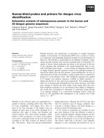
with a critical value a = 0.025. Figure 10.1 provides the Minitab computation for the

mean difference (1.489), the standard deviation of the mean differences (0.385), and
the Student’s t. The Student’s t statistic for the test can be computed as
t =

d
1.489
1.489
=
=
= 3.86
0.385
s d > 1n
1.926> 125

10.1 Tests of the Difference Between Two Normal Population Means: Dependent Samples

389


www.downloadslide.com

Figure 10.1 Hypothesis Testing for Differences Between New and Old
Turkey Weights
Paired T-Test and CI: New, Old
Paired T for New – old
N
New
25
old
25

Difference 25

Mean
19.732
18.244
1.489

StDev
3.226
2.057
1.926

SE Mean
0.645
0.411
0.385

95% lower bound for mean difference: 0.829
T-Test of mean difference = 0 (vs > 0): T-Value = 3.86 P-Value = 0.000

The computed value of Student’s t is greater than the critical value with a = 0.025 and
24 degrees of freedom, equal to 2.064 from the Student’s t table (Appendix Table 8).
From this analysis we see that there is strong evidence to conclude that the new
feeding method increases the weight of turkeys more than the old method.
Note also that the variance of the difference between the matched pairs could be
computed as follows (the correlation between the pairs is 0.823) using Equation 5.27:
S 2d = 1 0.411 22 + 1 0.645 22 - 2 * 1 0.823 21 0.411 21 0.645 2 = 0.146
S d = 0.385

This is the standard deviation of the differences as computed in the computer output.

EXERCISES
as m1 and process 2 has a mean defined as m2. The null
and alternative hypotheses are as follows:

Visit www.mymathlab.com/global or www.pearsonglobal
editions.com/newbold to access the data files.

Basic Exercises

H0 : m1 - m2 Ú 0

10.1

H1 : m1 - m2 6 0

You have been asked to determine if two different
production processes have different mean numbers
of units produced per hour. Process 1 has a mean
defined as m1 and process 2 has a mean defined
as m2. The null and alternative hypotheses are as
follows:

Using a random sample of 25 paired observations, the
standard deviation of the difference between sample
means is 25. Can you reject the null hypothesis using a
probability of Type I error a = 0.05 in each case?
a.
b.
c.

d.

H0 : m1 - m2 = 0
H1 : m1 - m2 7 0
Using a random sample of 25 paired observations, the
sample means are 50 and 60 for populations 1 and
2, respectively. Can you reject the null hypothesis
using a probability of Type I error a = 0.05 in each
case?
a.
b.
c.
d.
10.2

390

The sample standard deviation of the difference is 20
The sample standard deviation of the difference is 30
The sample standard deviation of the difference is 15
The sample standard deviation of the difference is 40

You have been asked to determine if two different
production processes have different mean numbers of
units produced per hour. Process 1 has a mean defined

Chapter 10

Two Population Hypothesis Tests

The sample means are 56 and 50
The sample means are 59 and 50
The sample means are 56 and 48
The sample means are 54 and 50

Application Exercises
10.3

In a study comparing banks in Germany and Great Britain, a sample of 145 matched pairs of banks was formed.
Each pair contained one bank from Germany and one
from Great Britain. The pairings were made in such a
way that the two members were as similar as possible
in regard to such factors as size and age. The ratio of total loans outstanding to total assets was calculated for
each of the banks. For this ratio, the sample mean difference (German – Great Britain) was 0.0518, and the
sample standard deviation of the differences was 0.3055.


www.downloadslide.com

10.4

Test, against a two-sided alternative, the null hypothesis
that the two population means are equal.
You have been asked to conduct a national study
of urban home selling prices to determine if there
has been an increase in selling prices over time. There has
been some concern that housing prices in major urban areas have not kept up with inflation over time. Your study
will use data collected from Atlanta, Chicago, Dallas, and
Oakland, which is contained in the data file House Selling Price. Formulate an appropriate hypothesis test and
use your statistical computer package to compute the appropriate statistics for analysis. Perform the hypothesis

test and indicate your conclusion.
Repeat the analysis using data from only the city of
Atlanta.

10.5

An agency offers preparation courses for a
graduate school admissions test to students. As
part of an experiment to evaluate the merits of the
course, 12 students were chosen and divided into 6
pairs in such a way that the members of any pair had
similar academic records. Before taking the test, one
member of each pair was assigned at random to take
the preparation course, while the other member did
not take a course. The achievement test scores are contained in the Student Pair data file. Assuming that the
differences in scores follow a normal distribution, test,
at the 5% level, the null hypothesis that the two population means are equal against the alternative that the
true mean is higher for students taking the preparation course.

10.2 T ESTS OF THE D IFFERENCE B ETWEEN T WO N ORMAL
P OPULATION M EANS : I NDEPENDENT S AMPLES
Two Means, Independent Samples, Known Population Variances
Now we consider the case where we have independent random samples from two normally distributed populations. The first population has a mean of mx and a variance of s2x
and we obtain a random sample of size nx. The second population has a mean of my and a
variance of s2y and we obtain a random sample of size ny.
In Section 8.2, we showed that if the sample means are denoted by x and y, then the
random variable
Z =

1 x - y 2 - 1 mx - my 2

s2y
s2x
+
A nx
ny

has a standard normal distribution. If the two population variances are known, tests of the difference between the population means can be based on this result, using the same arguments
as before. Generally, we are comfortable using known population variances if the process
being studied has been stable over some time and we have obtained similar variance measurements over this time. And because of the central limit theorem, the results presented here
hold for large sample sizes even if the populations are not normal. For large sample sizes, the
approximation is quite satisfactory when sample variances are used for population variances.
The appropriate tests are summarized in Equations 10.4, 10.5, and 10.6.

Tests of the Difference Between Population Means:
Independent Samples (Known Variances)
Suppose that we have independent random samples of nx and ny observations from normal distributions with means mx and my and variances s2x and
s2y, respectively. If the observed sample means are x and y, then the following tests have significance level a:
1. To test either null hypothesis
H0 : mx - my = 0 or H0 : mx - my … 0

against the alternative
H1 : mx - my 7 0

10.2 Tests of the Difference Between Two Normal Population Means: Independent Samples

391


www.downloadslide.com

the decision rule is as follows:
x - y

reject H0 if

s2y
s2x
A nx + ny

7 za

(10.4)

2. To test either null hypothesis
H0 : mx - my = 0 or H0 : mx - my Ú 0

against the alternative
H1 : mx - my 6 0

the decision rule is as follows:
reject H0 if

x - y
s2y
s2x
A nx + ny

6 - za

(10.5)

3. To test the null hypothesis
H0 : mx - my = 0

against the two-sided alternative
H1 : mx - my ? 0

the decision rule is as follows:
x - y

reject H0 if

s2y

s2x
A nx + ny

6 - z a>2 or

x - y
s2y
s2x
+
A nx
ny

7 z a>2

(10.6)

If the sample sizes are large (n 7 100), then a good approximation at significance level a can be made if we replace the population variances with the
sample variances. In addition, the central limit theorem leads to good approximations even if the populations are not normally distributed. The p-values for
all these tests are interpreted as the probability of getting a value at least as
extreme as the one obtained, given the null hypothesis.

Example 10.2 Comparison of Alternative Fertilizers
(Hypothesis Test for Differences Between Means)
Shirley Brown, an agricultural economist, wants to compare cow manure and turkey
dung as fertilizers. Historically, farmers had used cow manure on their cornfields.
Recently, a major turkey farmer offered to sell composted turkey dung at a favorable
price. The farmers decided that they would use this new fertilizer only if there was
strong evidence that productivity increased over the productivity that occurred with
cow manure. Shirley was asked to conduct the research and statistical analysis in order
to develop a recommendation to the farmers.
Solution To begin the study, Shirley specified a hypothesis test with
H0 : mx - my … 0
versus the alternative that
H1 : mx - my 7 0

392

Chapter 10

Two Population Hypothesis Tests


www.downloadslide.com

where mx is the population mean productivity using turkey dung and my is the
population mean productivity using cow manure. H1 indicates that turkey dung results

in higher productivity. The farmers will not change their fertilizer unless there is strong
evidence in favor of increased productivity. She decided before collecting the data that
a significance level of a = 0.05 would be used for this test.
Using this design, Shirley implemented an experiment to test the hypothesis. Cow
manure was applied to one set of ny = 25 randomly selected fields. The sample mean
productivity was y = 100. From past experience the variance in productivity for these
fields was assumed to be s2y = 400. Turkey dung was applied to a second random sample of nx = 25 fields, and the sample mean productivity was x = 115. Based on published research reports, the variance for these fields was assumed to be s2x = 625. The
two sets of random samples were independent. The decision rule is to reject H0 in favor
of H1 if
x - y
s2y
A nx + ny

7 za

s2x

The computed statistics for this problem are as follows:
nx = 25 x = 115 s2x = 625
ny = 25 y = 100 s2y = 400
115 - 100
z =
= 2.34
625
400
+
A 25
25
Comparing the computed value of z = 2.34 with z 0.05 = 1.645, Shirley concluded that
the null hypothesis is clearly rejected. In fact, we found that the p-value for this test is

0.0096. As a result, there is overwhelming evidence that turkey dung results in higher
productivity than cow manure.

Two Means, Independent Samples, Unknown Population
Variances Assumed to Be Equal
In those cases where the population variances are not known and the sample sizes are
under 100, we need to use the Student’s t distribution. There are some theoretical problems when we use the Student’s t distribution for differences between sample means.
However, these problems can be solved using the procedure that follows if we can assume
that the population variances are equal. This assumption is realistic in many cases where
we are comparing groups. In Section 10.4 we present a procedure for testing the equality
of variances from two normal populations.
The major difference is that this procedure uses a commonly pooled estimator of the
equal population variance. This estimator is as follows:
s 2p =

1 nx - 1 2s 2x + 1 ny - 1 2s 2y
1 nx + ny - 2 2

The degrees of freedom for s 2p and for the Student’s t statistic below is nx + ny - 2. The
hypothesis test is performed using the Student’s t statistic for the difference between two
means:
t =

1 x - y 2 - 1 mx - my 2
s 2p
s 2p
+
A nx
ny

10.2 Tests of the Difference Between Two Normal Population Means: Independent Samples

393


www.downloadslide.com

Note that the form for the test statistic is similar to that of the Z statistic, which is used
when the population variances are known. The various tests using this procedure are
summarized next.

Tests of the Difference Between Population Means:
Population Variances Unknown and Equal
In these tests it is assumed that we have an independent random sample of
size nx and ny observations drawn from normally distributed populations with
means mx and my and a common variance. The sample variances s 2x and s 2y are
used to compute a pooled variance estimator:
s 2p =

1 nx - 1 2s 2x + 1 ny - 1 2s 2y
1 nx + ny - 2 2

(10.7)

We emphasize here that s p2 is the weighted average of the two sample variances, s x2 and s 2y.
Then, using the observed sample means x and y, the following tests have
significance level a:
1. To test either null hypothesis
H0 : mx - my = 0 or H0 : mx - my … 0

against the alternative
H1 : mx - my 7 0

the decision rule is as follows:
reject H0 if

x - y
s 2p
s 2p
A nx + ny

7 tnx + ny - 2,a

(10.8)

2. To test either null hypothesis
H0 : mx - my = 0 or H0 : mx - my Ú 0

against the alternative
H1 : mx - my 6 0

the decision rule is as follows:
reject H0 if

x - y
s 2p
s 2p
A nx + ny

6 - tnx + ny - 2,a

(10.9)

3. To test the null hypothesis
H0 : mx - my

against the two-sided alternative
H1 : mx - my ? 0

the decision rule is as follows:
reject H0 if

394

Chapter 10

x - y
s 2p
s 2p
+
A nx
ny

Two Population Hypothesis Tests

6 - tnx + ny - 2,a>2 or

x - y
s 2p
s 2p

+
A nx
ny

7 tnx + ny - 2,a>2

(10.10)


www.downloadslide.com

Here, tnx + ny - 2,a is the number for which

P 1 tnx + ny - 2 7 tnx + ny - 2,a 2 = a

Note that the degrees of freedom for the Student’s t is nx + ny - 2 for all of
these tests.
We interpret p-values for all these tests as the probability of getting a value
as extreme as the one obtained, given the null hypothesis.

Example 10.3 Retail Sales Patterns (Hypothesis
Test for Differences Between Means)
A sporting goods store operates in a medium-sized shopping mall. In order to plan
staffing levels, the manager has asked for your assistance to determine if there is strong
evidence that Monday sales are higher than Saturday sales.
Solution To answer the question, you decide to gather random samples of 25
Saturdays and 25 Mondays from a population of several years of data. The samples are
drawn independently. You decide to test the null hypothesis
H0 : mM - mS … 0
against the alternative hypothesis

H1 : mM - mS 7 0
where the subscripts M and S refer to Monday and Saturday sales. The sample statistics
are as follows:
xM = 1078 s M = 633 nM = 25
yS = 908.2 s S = 469.8 nS = 25
The pooled variance estimate is as follows:
s 2p =

1 25 - 1 21 633 22 + 1 25 - 1 21 469.8 22
= 310,700
25 + 25 - 2

The test statistic is then computed as follows:
t =

xM - yS
s 2p
s 2p
+
A nx
ny

=

1078 - 908.2
= 1.08
310,700
310,700
+
A 25

25

Using a significance level of a = 0.05 and 48 degrees of freedom, we find that the critical value of t is 1.677. Therefore, we conclude that there is not sufficient evidence to
reject the null hypothesis, and, thus, there is no reason to conclude that mean sales on
Mondays are higher.

Example 10.4 Analysis of Alternative
Turkey-Feeding Programs (Hypothesis
Test for Differences Between Means)
In this example we revisit the turkey-feeding problem from Example 10.1. In that
example we used a matched-pairs test and concluded that the new feeding program did
result in greater weight gain than the old program, using a = 0.025. In this example we

10.2 Tests of the Difference Between Two Normal Population Means: Independent Samples

395


www.downloadslide.com

solve the same problem. The hypothesis test from Example 10.1 is exactly the same in
this example. However, here we assume that the two samples are independent and we
do not have matched pairs. We use the same data file, Turkey Feeding, which contains
the sample of weights for the old and new feeding programs.
Solution This solution follows the same general approach as seen in Example 10.1.
However, we assume that we have independent random samples from populations
with equal variances. Figure 10.2 contains the computer computation of the statistics
needed to test the hypothesis. Note that the difference in sample means is still 1.489,
but the pooled standard deviation for the difference is substantially larger at 2.7052:
s 2d = a

2.7052 2
2.7052 2
b + a
b = 0.585
125
125

s d = 0.765
and the resulting computed Student’s t is
t =

1.489
= 1.946
0.765

Figure 10.2 Turkey Weight Study: Independent Samples, Population Variances
Equal (Minitab Output)
Two-Sample T-Test and CI: New, Old
Two-sample T for New vs old
New
old

N
25
25

Mean
19.73
18.24

StDev
3.23
2.06

SE Mean
0.65
0.41

Difference 5 mu (New) 2 mu (Old)
Estimate for difference: 1.489
95% lower bound for difference: 0.205
T-Test of difference 5 0 (vs .): T-Value 5 1.95 P-Value 5 0.029 DF 5 48
Both use Pooled StDev 5 2.7052

Since the degrees of freedom with the independent samples assumption is 48, the critical value of the Student’s t is 2.01, with a = 0.025. The computed value is smaller, and
we cannot reject the null hypothesis; thus we cannot conclude that the new feeding
process results in a greater weight gain. Note that since the variance and standard deviation are larger, the resulting test does not have the same power. In Example 10.1 the
p-value for the hypothesis test with paired observations was 0.00, whereas in Example
10.4, assuming independent samples, the p-value was 0.029.

Two Means, Independent Samples, Unknown Population
Variances Not Assumed to Be Equal
Hypothesis tests of differences between population means when the individual variances are unknown and not equal require modification of the variance computation and
the degrees of freedom. The computation of sample variance for the difference between
sample means is changed. There are substantial complexities in the determination of
degrees of freedom for the critical value of the Student’s t statistic. The specific computational forms were presented in Section 8.2. Equations 10.11–10.14 summarize the
procedures.

396

Chapter 10

Two Population Hypothesis Tests


www.downloadslide.com

Tests of the Difference Between Population
Means: Population Variances Unknown
and Not Equal
These tests assume that we have independent random samples of size nx and
ny observations from normal populations with means mx and my and unequal
variances. The sample variances s x2 and s 2y are used. The number of degrees of
freedom v for the Student’s t statistic is given by the following:
ca
v =

s 2y 2
s 2x
b + a bd
nx
ny

(10.11)

s 2y 2
s 2x 2
a b > 1 nx - 1 2 + a b > 1 ny - 1 2
nx

ny

Then, using the observed sample means x and y, the following tests have significance level a:
1. To test either null hypothesis
H0 : mx - my = 0 or H0 : mx - my … 0

against the alternative
H1 : mx - my 7 0

the decision rule is as follows:
x - y

reject H0 if

s 2y
s 2x
A nx + ny

7 tv,a

(10.12)

2. To test either null hypothesis
H0 : mx - my = 0 or H0 : mx - my Ú 0

against the alternative
H1 : mx - my 6 0

the decision rule is as follows:
reject H0 if

x - y
s 2y
s 2x
+
A nx
ny

6 - tv,a

(10.13)

3. To test the null hypothesis
H0 : mx - my = 0

against the two-sided alternative
H1 : mx - my ? 0

the decision rule is as follows:
reject H0 if

x - y
s 2y
s 2x
A nx + ny

6 - tv,a>2 or

x - y
s 2y

s 2x
A nx + ny

7 tv,a>2

(10.14)

Here, tv,a is the number for which

P1 tv 7 tv,a 2 = a

10.2 Tests of the Difference Between Two Normal Population Means: Independent Samples

397


www.downloadslide.com

The analysis for Example 10.4 was run again without assuming equal population variances. The computer output is shown in Figure 10.3. The computational results are all the
same except that the degrees of freedom are now 40 instead of 48 when we assumed that
the variances were equal in Example 10.4. The change in critical value of the Student’s t is
so small that the p-value did not change. And we still do not have evidence to reject the
null hypothesis and cannot conclude that the new program results in greater weight gain.
Figure 10.3

Two-Sample T-Test and CI: New, Old

Turkey Weight
Study: Independent
Samples, Population

Variances not
Assumed Equal

Two-sample T for New vs old
New
old

N
25
25

Mean
19.73
18.24

StDev
3.23
2.06

SE Mean
0.65
0.41

Difference 5 mu (New) 2 mu (Old)
Estimate for difference: 1.489
95% lower bound for difference: 0.200
T-Test of difference 5 0 (vs .): T-Value 5 1.95 P-Value 5 0.029 DF 5 40

EXERCISES
Basic Exercises

10.6

H0 : m1 - m2 = 0
H1 : m1 - m2 7 0
Use a random sample of 25 observations from process
1 and 28 observations from process 2 and the known
variance for process 1 equal to 900 and the known variance for process 2 equal to 1,600. Can you reject the null
hypothesis using a probability of Type I error a = 0.05
in each case?
a.
b.
c.
d.
10.7

The process means are 50 and 60.
The difference in process means is 20.
The process means are 45 and 50.
The difference in process means is 15.

You have been asked to determine if two different
production processes have different mean numbers
of units produced per hour. Process 1 has a mean defined as m1 and process 2 has a mean defined as m2.
The null and alternative hypotheses are as follows:
H0 : m1 - m2 … 0
H1 : m1 - m2 7 0
The process variances are unknown but assumed to
be equal. Using random samples of 25 observations
from process 1 and 36 observations from process 2, the
sample means are 56 and 50 for populations 1 and 2,

respectively. Can you reject the null hypothesis using
a probability of Type I error a = 0.05 in each case?
a. The sample standard deviation from process 1 is 30
and from process 2 is 28.

398

b. The sample standard deviation from process 1 is 22
and from process 2 is 33.
c. The sample standard deviation from process 1 is 30
and from process 2 is 42.
d. The sample standard deviation from process 1 is 15
and from process 2 is 36.

You have been asked to determine if two different
production processes have different mean numbers
of units produced per hour. Process 1 has a mean defined as m1 and process 2 has a mean defined as m2.
The null and alternative hypotheses are as follows:

Chapter 10

Two Population Hypothesis Tests

Application Exercises
10.8

A screening procedure was designed to measure attitudes toward minorities as managers. High scores indicate negative attitudes and low scores indicate positive
attitudes. Independent random samples were taken of
151 male financial analysts and 108 female financial
analysts. For the former group the sample mean and

standard deviation scores were 85.8 and 19.13, whereas
the corresponding statistics for the latter group were
71.5 and 12.2. Test the null hypothesis that the two
population means are equal against the alternative that
the true mean score is higher for male than for female
financial analysts.
10.9 For a random sample of 125 British entrepreneurs, the
mean number of job changes was 1.91 and the sample
standard deviation was 1.32. For an independent random sample of 86 British corporate managers, the
mean number of job changes was 0.21 and the sample
standard deviation was 0.53. Test the null hypothesis
that the population means are equal against the alternative that the mean number of job changes is higher
for British entrepreneurs than for British corporate
managers.
10.10 A political science professor is interested in comparing the characteristics of students who do and do not
vote in national elections. For a random sample of 114
students who claimed to have voted in the last presidential election, she found a mean grade point average of 2.71 and a standard deviation of 0.64. For an
independent random sample of 123 students who did


www.downloadslide.com
not vote, the mean grade point average was 2.79 and
the standard deviation was 0.56. Test, against a twosided alternative, the null hypothesis that the population means are equal.
10.11 In light of a recent large corporation bankruptcy,
auditors are becoming increasingly concerned about
the possibility of fraud. Auditors might be helped
in determining the chances of fraud if they carefully measure cash flow. To evaluate this possibility, samples of midlevel auditors from CPA firms
were presented with cash-flow information from
a fraud case, and they were asked to indicate the
chance of material fraud on a scale from 0 to 100.

A random sample of 36 auditors used the cash-flow
information. Their mean assessment was 36.21,
and the sample standard deviation was 22.93. For
an independent random sample of 36 auditors not
using the cash-flow information, the sample mean
and standard deviation were, respectively, 47.56
and 27.56. Assuming that the two population distributions are normal with equal variances, test,
against a two-sided alternative, the null hypothesis
that the population means are equal.
10.12 The recent financial collapse has led to considerable
concern about the information provided to potential investors. The government and many researchers
have pointed out the need for increased regulation of
financial offerings. The study in this exercise concerns

the effect of sales forecasts on initial public offerings.
Initial public offerings’ prospectuses were examined.
In a random sample of 70 prospectuses in which sales
forecasts were disclosed, the mean debt-to-equity ratio
prior to the offering issue was 3.97, and the sample
standard deviation was 6.14. For an independent random sample of 51 prospectuses in which sales earnings
forecasts were not disclosed, the mean debt-to-equity
ratio was 2.86, and the sample standard deviation was
4.29. Test, against a two-sided alternative, the null
hypothesis that population mean debt-to-equity ratios
are the same for disclosers and nondisclosers of earnings forecasts.
10.13 A publisher is interested in the effects on sales of
college texts that include more than 100 data files.
The publisher plans to produce 20 texts in the business area and randomly chooses 10 to have more
than 100 data files. The remaining 10 are produced
with at most 100 data files. For those with more than

100, first-year sales averaged 9,254, and the sample
standard deviation was 2,107. For the books with at
most 100, average first-year sales were 8,167, and the
sample standard deviation was 1,681. Assuming that
the two population distributions are normal with
the same variance, test the null hypothesis that the
population means are equal against the alternative
that the true mean is higher for books with more than
100 data files.

10.3 T ESTS OF THE D IFFERENCE B ETWEEN T WO P OPULATION
P ROPORTIONS (L ARGE S AMPLES )
Next, we develop procedures for comparing two population proportions. We consider a
standard model with a random sample of nx observations from a population with a proportion Px of successes and a second independent random sample of ny observations from
a population with a proportion Py of successes.
In Chapter 5 we saw that, for large samples, proportions can be approximated as normally distributed random variables, and, as a result,
1 pnx - pny 2 - 1 Px - Py 2

Z =
A

Py1 1 - Py 2
Px1 1 - Px 2
+
nx
ny

has a standard normal distribution.
We want to test the hypothesis that the population proportions Px and Py are equal.
H0 : Px - Py = 0 or H0 : Px = Py

Denote their common value by P0. Then under this hypothesis
1 pnx - pny 2

Z =
A

P01 1 - P0 2
P01 1 - P0 2
+
nx
ny

follows to a close approximation a standard normal distribution.

10.3 Tests of the Difference Between Two Population Proportions (Large Samples)

399


www.downloadslide.com

Finally, the unknown proportion P0 can be estimated by a pooled estimator defined
as follows:
pn0 =

nxpnx + nypny
nx + ny

The null hypothesis in these tests assumes that the population proportions are equal. If

the null hypothesis is true, then an unbiased and efficient estimator for P0 can be obtained
by combining the two random samples, and, as a result, pn0 is computed using this equation. Then, we can replace the unknown P0 by pn0 to obtain a random variable that has a
distribution close to the standard normal for large sample sizes.
The tests are summarized as follows.

Testing the Equality of Two Population Proportions
(Large Samples)
We are given independent random samples of size nx and ny with proportion
of successes pnx and pny. When we assume that the population proportions are
equal, an estimate of the common proportion is as follows:
pn0 =

nxpnx + nypny
nx + ny

For large sample sizes—nP0(1 - P0) 7 5—the following tests have significance
level a:
1. To test either null hypothesis
H0 : Px - Py = 0 or H0 : Px - Py … 0

against the alternative
H1 : Px - Py 7 0

the decision rule is as follows:
1 pnx - pny 2

reject H0 if
A

pn01 1 - pn0 2

nx

+

pn01 1 - pn0 2

7 za

(10.15)

ny

2. To test either null hypothesis
H0 : Px - Py = 0 or H0 : Px - Py Ú 0

against the alternative
H1 : Px - Py 6 0

the decision rule is as follows:
reject H0 if

1 pnx - pny 2
pn01 1 - pn0 2
pn01 1 - pn0 2
+
A
nx
ny

3. To test the null hypothesis

H0 : Px - Py = 0

against the two-sided alternative
H1 : Px - Py ? 0

400

Chapter 10

Two Population Hypothesis Tests

6 - za

(10.16)


www.downloadslide.com

the decision rule is as follows:
1 pnx - pny 2

reject H0 if
A

pn01 1 - pn0 2
nx

+

pn01 1 - pn0 2

1 pnx - pny 2

6 - z a>2 or

ny

pn01 1 - pn0 2
pn01 1 - pn0 2
+
A
nx
ny

7 z a>2

(10.17)

It is also possible to compute and interpret p-values as the probability
of getting a value at least as extreme as the one obtained, given the null
hypothesis.

Example 10.5 Change in Customer Recognition
of New Products After an Advertising Campaign
(Hypothesis Tests of Differences Between
Proportions)
Northern States Marketing Research has been asked to determine if an advertising
campaign for a new cell phone increased customer recognition of the new World A
phone. A random sample of 270 residents of a major city were asked if they knew about
the World A phone before the advertising campaign. In this survey 50 respondents

had heard of World A. After the advertising campaign, a second random sample of 203
residents were asked exactly the same question using the same protocol. In this case 81
respondents had heard of the World A phone. Do these results provide evidence that
customer recognition increased after the advertising campaign?
Solution Define Px and Py as the population proportions that recognized the
World A phone before and after the advertising campaign, respectively. The null
hypothesis is
H0 : Px - Py Ú 0
and the alternative hypothesis is
H1 : Px - Py 6 0
The null hypothesis states that there was no increase in the proportion that recognized the new phone after the advertising campaign and the alternative hypothesis
states that there was an increase.
The decision rule is to reject H0 in favor of H1 if

1 pn x - pn y 2

pn 01 1 - pn 0 2
pn 01 1 - pn 0 2
+
A
nx
ny

6 -z a

The data for this problem are as follows:
nx = 270 pnx = 50>270 = 0.185 ny = 203 pny = 81>203 = 0.399
The estimate of the common variance P0 under the null hypothesis is as follows:
pn0 =

nxpnx + nypny
n x + ny

=

1 270 21 0.185 2 + 1 203 21 0.399 2
= 0.277
270 + 203

10.3 Tests of the Difference Between Two Population Proportions (Large Samples)

401


www.downloadslide.com

The test statistic is as follows:

1 pnx - pny 2

pn01 1 - pn0 2
pn01 1 - pn0 2
+
A
nx
ny

=

0.185 - 0.399

1 0.277 21 1 - 0.277 2
1 0.277 21 1 - 0.277 2
+
A
270
203

= -5.15

For a one-tailed test with a = 0.05, the -z 0.05 value is -1.645. Thus, since -5.15 6
-1.645, we reject the null hypothesis and conclude that customer recognition did increase after the advertising campaign.

EXERCISES
Basic Exercise
10.14 Test the hypotheses
H0 : Px - Py = 0

10.18

H1 : Px - Py 6 0
using the following statistics from random samples.
a. pnx = 0.42, nx = 500;
pny = 0.50, ny = 600
b. pnx = 0.60, nx = 500;
pny = 0.64, ny = 600
c. pnx = 0.42, nx = 500;
pny = 0.49, ny = 600
d. pnx = 0.25, nx = 500;
pny = 0.34, ny = 600

e. pnx = 0.39, nx = 500;
pny = 0.42, ny = 600

10.19

Application Exercises
10.15 Random samples of 900 people in the United States
and in Great Britain indicated that 60% of the people
in the United States were positive about the future
economy, whereas 66% of the people in Great Britain
were positive about the future economy. Does this
provide strong evidence that the people in Great Britain are more optimistic about the economy?
10.16 A random sample of 1,556 people in country A were
asked to respond to this statement: Increased world
trade can increase our per capita prosperity. Of these sample members, 38.4% agreed with the statement. When
the same statement was presented to a random sample of 1,108 people in country B, 52.0% agreed. Test
the null hypothesis that the population proportions
agreeing with this statement were the same in the two
countries against the alternative that a higher proportion agreed in country B.
10.17 Small-business telephone users were surveyed
6 months after access to carriers other than AT&T
became available for wide-area telephone service. Of
a random sample of 368 users, 92 said they were attempting to learn more about their options, as did
37 of an independent random sample of 116 users of

402

Chapter 10

Two Population Hypothesis Tests

10.20

10.21

alternative carriers. Test, at the 5% significance level
against a two-sided alternative, the null hypothesis
that the two population proportions are the same.
Employees of a building materials chain facing a
shutdown were surveyed on a prospective employee
ownership plan. Some employees pledged $10,000 to
this plan, putting up $800 immediately, while others
indicated that they did not intend to pledge. Of a random sample of 175 people who had pledged, 78 had
already been laid off, whereas 208 of a random sample
of 604 people who had not pledged had already been
laid off. Test, at the 5% level against a two-sided alternative, the null hypothesis that the population proportions already laid off were the same for people who
pledged as for those who did not.
Of a random sample of 381 high-quality investment
equity options, 191 had less than 30% debt. Of an independent random sample of 166 high-risk investment equity options, 145 had less than 30% debt. Test,
against a two-sided alternative, the null hypothesis
that the two population proportions are equal.
Two different independent random samples of consumers were asked about satisfaction with their computer system each in a slightly different way. The
options available for answer were slightly different
in the two cases. When asked how satisfied they were
with their computer system, 138 of the first group of
240 sample members opted for “very satisfied.” When
the second group was asked how dissatisfied they
were with their computer system, 128 of 240 sample
members opted for very satisfied. Test, at the 5% significance level against the obvious one-sided alternative, the null hypothesis that the two population
proportions are equal.

Of a random sample of 1,200 people in Denmark, 480
had a positive attitude toward car salespeople. Of
an independent random sample of 1,000 people in
France, 790 had a positive attitude toward car salespeople. Test, at the 1% level the null hypothesis that
the population proportions are equal, against the
alternative that a higher proportion of French have a
positive attitude toward car salespeople.


www.downloadslide.com

10.4 T ESTS OF THE E QUALITY OF THE V ARIANCES B ETWEEN
T WO N ORMALLY D ISTRIBUTED P OPULATIONS
There are a number of situations in which we are interested in comparing the variances
from two normally distributed populations. For example, the Student’s t test in Section
10.2 assumed equal variances and used the two sample variances to compute a pooled
estimator for the common variances. Quality-control studies are often concerned with the
question of which process has the smaller variance.
In this section we develop a procedure for testing the assumption that population
variances from independent samples are equal. To perform such tests, we introduce the
F probability distribution. We begin by letting s 2x be the sample variance for a random
sample of nx observations from a normally distributed population with population variance s2x. A second independent random sample of size ny provides a sample variance of s 2y
from a normal population with population variance s2y. Then the random variable
F =

s 2x >s2x
s 2y >s2y

follows a distribution known as the F distribution. This family of distributions, which is
widely used in statistical analysis, is identified by the degrees of freedom for the numerator and the degrees of freedom for the denominator. The number of degrees of freedom

for the numerator is associated with the sample variance s 2x and equal to 1 nx - 1 2. Similarly, the number of degrees of freedom for the denominator is associated with the sample
variance s 2y and equal to 1 ny - 1 2.
The F distribution is constructed as the ratio of two chi-square random variables, each
divided by its degrees of freedom. The chi-square distribution relates the sample and
population variances for a normally distributed population. Hypothesis tests that use the
F distribution depend on the assumption of a normal distribution. The characteristics of
the F distribution are summarized next.

The F Distribution
We have two independent random samples with nx and ny observations from
two normal populations with variances s2x and sy2. If the sample variances are
s x2 and s y2, then the random variable
F =

s 2x >s2x
s 2y >s2y

(10.18)

has an F distribution with numerator degrees of freedom (nx - 1) and
denominator degrees of freedom (ny - 1).
An F distribution with numerator degrees of freedom v1 and denominator degrees of freedom v2 is denoted Fv1,v2. We denote as Fv1,v2,a the number for which
P 1 Fv1,v2 7 Fv1,v2,a 2 = a

We need to emphasize that this test is quite sensitive to the assumption of
normality.
The cutoff points for Fv1,v2,a, for a equal to 0.05 and 0.01, are provided in Appendix Table 9.
For example, for 10 numerator degrees of freedom and 20 denominator degrees of freedom,
we see from the table that
F10,20,0.05 = 2.348 and F10,20,0.01 = 3.368

Hence,
P1 F10,20 7 2.348 2 = 0.05 and P1 F10,20 7 3.368 2 = 0.01

Figure 10.4 presents a schematic description of the F distribution for this example.

10.4 Tests of the Equality of the Variances Between Two Normally Distributed Populations

403


www.downloadslide.com

Figure 10.4
F Probability Density
Function with 10
Numerator Degrees
of Freedom and
20 Denominator
Degrees of Freedom

a 5 0.05
0

1

2

2.348

3

4 F

In practical applications we usually arrange the F ratio so that the larger sample variance is in the numerator and the smaller is in the denominator. Thus, we need to use only
the upper cutoff points to test the hypothesis of equality of variances. When the population variances are equal, the F random variable becomes
F =

s 2x
s 2y

and this ratio of sample variances becomes the test statistic. The intuition for this test is
quite simple: If one of the sample variances greatly exceeds the other, then we must conclude that the population variances are not equal. The hypothesis tests of equality of variances are summarized as follows.

Tests of Equality of Variances from Two
Normal Populations
Let s x2 and s y2 be observed sample variances from independent random samples of
size nx and ny from normally distributed populations with variances s2x and s2y. Use
s x2 to denote the larger variance. Then the following tests have significance level a:
1. To test either null hypothesis
H0 : s2x = s2y or H0 : s2x … s2y

against the alternative
H1 : s2x 7 s2y

the decision rule is as follows:
reject H0 if F =

s 2x
s 2y

7 Fnx - 1,ny - 1,a

(10.19)

2. To test the null hypothesis
H0 : s2x = s2y

against the two-sided alternative
H1 : s2x ? s2y

the decision rule is as follows:
reject H0 if F =

s 2x
s 2y

7 Fnx - 1,ny - 1,a>2

(10.20)

where s x2 is the larger of the two sample variances. Since either sample
variance could be larger, this rule is actually based on a two-tailed test,
and, hence, we use a>2 as the upper-tail probability.
Here, Fnx - 1, ny - 1 is the number for which
P 1 Fnx - 1,ny - 1 7 Fnx - 1,ny - 1,a 2 = a

where Fnx - 1, ny - 1 has an F distribution with (nx - 1) numerator degrees of
freedom and (ny - 1) denominator degrees of freedom.

404

Chapter 10

Two Population Hypothesis Tests


www.downloadslide.com

For all these tests a p-value is the probability of getting a value at least as
extreme as the one obtained, given the null hypothesis. Because of the complexity of the F distribution, critical values are computed for only a few special
cases. Thus, p-values will be typically computed using a statistical package
such as Minitab.

Example 10.6 Study of Maturity Variances
(Hypothesis Tests for the Equality of Two Variances)
The research staff of Investors Now, an online financial trading firm, was interested in
determining if there is a difference in the variance of the maturities of AAA-rated industrial bonds compared to CCC-rated industrial bonds.
Solution This question requires that we design a study that compares the population
variances of maturities for the two different bonds. We will test the null hypothesis
H0 : s2x = s2y
against the alternative hypothesis
H1 : s2x ? s2y
where s2x is the variance in maturities for AAA-rated bonds and s2y is the variance
in maturities for CCC-rated bonds. The significance level of the test was chosen as
a = 0.02.
The decision rule is to reject H0 in favor of H1 if
s 2x
s 2y

7 Fnx - 1,ny - 1,a>2

Note here that either sample variance could be larger, and we place the larger sample variance in the numerator. Hence, the probability for this upper tail is a>2. A random sample of 17 AAA-rated bonds resulted in a sample variance s 2x = 123.35, and
an independent random sample of 11 CCC-rated bonds resulted in a sample variance
s 2y = 8.02. The test statistic is as follows:
s 2x
s 2y

=

123.35
= 15.380
8.02

Given a significance level of a = 0.02, we find that the critical value of F, from interpolation in Appendix Table 9, is as follows:
F16,10,0.01 = 4.520
Clearly, the computed value of F (15.380) exceeds the critical value (4.520), and we reject H0 in favor of H1. Thus, there is strong evidence that variances in maturities are different for these two types of bonds.

EXERCISES
Basic Exercise

using the following data.

10.22 Test the hypothesis

a. s 2x = 125, ny = 45; s 2y = 51, ny = 41
H0 : s2x = s2y

b. s 2x = 125, ny = 45; s 2y = 235, ny = 44

H1 : s2x 7 s2y

c. s 2x = 134, ny = 48; s 2y = 51, ny = 41
d. s 2x = 88, ny = 39; s 2y = 167, ny = 25

Exercises

405


www.downloadslide.com

Application Exercises
10.23 It is hypothesized that the more expert a group of people
examining personal income tax filings, the more variable
the judgments will be about the accuracy. Independent
random samples, each of 30 individuals, were chosen from groups with different levels of expertise. The
low-expertise group consisted of people who had just
completed their first intermediate accounting course.
Members of the high-expertise group had completed
undergraduate studies and were employed by reputable CPA firms. The sample members were asked to
judge the accuracy of personal income tax filings. For the
low-expertise group, the sample variance was 451.770,
whereas for the high-expertise group, it was 1,614.208.
Test the null hypothesis that the two population variances are equal against the alternative that the true
variance is higher for the high-expertise group.
10.24 It is hypothesized that the total sales of a corporation
should vary more in an industry with active price
competition than in one with duopoly and tacit collusion. In a study of the merchant ship production
industry it was found that in 4 years of active price

competition, the variance of company A’s total sales
was 114.09. In the following 7 years, during which
there was duopoly and tacit collusion, this variance
was 16.08. Assume that the data can be regarded as
an independent random sample from two normal
distributions. Test, at the 5% level, the null hypothesis
that the two population variances are equal against
the alternative that the variance of total sales is higher
in years of active price competition.
10.25 In light of a number of recent large-corporation bankruptcies, auditors are becoming increasingly concerned
about the possibility of fraud. Auditors might be helped
in determining the chances of fraud if they carefully
measure cash flow. To evaluate this possibility, samples
of midlevel auditors from CPA firms were presented
with cash-flow information from a fraud case, and they

10.5 S OME C OMMENTS

ON

were asked to indicate the chance of material fraud on
a scale from 0 to 100. A random sample of 36 auditors
used the cash-flow information. Their mean assessment
was 36.21, and the sample standard deviation was 22.93.
For an independent random sample of 36 auditors not
using the cash-flow information, the sample mean and
standard deviation were respectively 47.56 and 27.56.
Test the assumption that population variances for
assessments of the chance of material fraud were the
same for auditors using cash-flow information as for

auditors not using cash-flow information against a
two-sided alternative hypothesis.
10.26 A publisher is interested in the effects on sales of college texts that include more than 100 data files. The
publisher plans to produce 20 texts in the business
area and randomly chooses 10 to have more than 100
data files. The remaining 10 are produced with at most
100 data files. For those with more than 100, first-year
sales averaged 9,254, and the sample standard deviation was 2,107. For the books with at most 100, average
first-year sales were 8,167, and the sample standard
deviation was 1,681. Assuming that the two population distributions are normal, test the null hypothesis
that the population variances are equal against the
alternative that the population variance is higher for
books with more than 100 data files.
10.27 A university research team was studying the relationship between idea generation by groups with
and without a moderator. For a random sample of
four groups with a moderator, the mean number of
ideas generated per group was 78.0, and the standard
deviation was 24.4. For a random sample of four
groups without a moderator, the mean number of
ideas generated was 63.5, and the standard deviation
was 20.2. Test the assumption that the two population variances were equal against the alternative that
the population variance is higher for groups with a
moderator.

H YPOTHESIS T ESTING

In this chapter we have presented several important applications of hypothesis-testing
methodology. In an important sense, this methodology is fundamental to decision making and analysis in the face of random variability. As a result, the procedures have great
applicability to a number of research and management decisions. The procedures are relatively easy to use, and various computer processes minimize the computational effort.
Thus, we have a tool that is appealing and quite easy to use. However, there are some

subtle problems and areas of concern that we need to consider to avoid serious mistakes.
The null hypothesis plays a crucial role in the hypothesis-testing framework. In a typical investigation we set the significance level, a, at a small probability value. Then, we
obtain a random sample and use the data to compute a test statistic. If the test statistic is
outside the acceptance region (depending on the direction of the test), the null hypothesis
is rejected and the alternative hypothesis is accepted. When we do reject the null hypothesis, we have strong evidence—a small probability of error—in favor of the alternative
hypothesis. In some cases we may fail to reject a drastically false null hypothesis simply
because we have only limited sample information or because the test has low power. A test
with low power usually results from a small sample size, poor measurement procedures,
a large variance in the underlying population, or some combination of these factors. There
406

Chapter 10

Two Population Hypothesis Tests


www.downloadslide.com

may be important cases where this outcome is appropriate. For example, we would not
change an existing process that is working effectively unless we had strong evidence that
a new process clearly would be better. In other cases, however, the special status of the
null hypothesis is neither warranted nor appropriate. In those cases we might consider
the costs of making both Type I and Type II errors in a decision process. We might also
consider a different specification of the null hypothesis—noting that rejection of the null
provides strong evidence in favor of the alternative. When we have two alternatives, we
could initially choose either as the null hypothesis. In the cereal-package-weight example
at the beginning of Chapter 9, the null hypothesis could be either that
H0 : m Ú 16

or that

H0 : m … 16

In the first case rejection would provide strong evidence that the population mean weight is
less than 16. In the latter case rejection would provide strong evidence that the population
mean weight is greater than 16. As we have indicated, failure to reject either of these null
hypotheses would not provide strong evidence. There are also procedures for controlling
both Type I and Type II errors simultaneously (see, for example, Carlson and Thorne 1997).
Our work in Chapter 10 considers null hypotheses for the differences between population means of the form
H0 : m1 - m2 Ú 16

or
H0 : m1 - m2 … 16

The entire discussion here applies similarly to hypothesis tests on the difference between
population means.
On some occasions very large amounts of sample information are available, and
we reject the null hypothesis even when differences are not practically important. Thus,
we need to contrast statistical significance with a broader definition of significance.
Suppose that very large samples are used to compare annual mean family incomes in two
cities. One result might be that the sample means differ by $2.67, and that difference might
lead us to reject a null hypothesis and thus conclude that one city has a higher mean family
income than the other. Although that result might be statistically significant, it clearly has
no practical significance with respect to consumption or quality of life.
In specifying a null hypothesis and a testing rule, we are defining the test conditions
before we look at the sample data that were generated by a process that includes a random
component. Thus, if we look at the data before defining the null and alternative hypotheses, we no longer have the stated probability of error, and the concept of “strong evidence”
resulting from rejecting the null hypothesis is not valid. For example, if we decide on the
significance level of our test after we have seen the p-values, then we cannot interpret our
results in probability terms. Suppose that an economist compares each of five different income-enhancing programs against a standard minimal level using a hypothesis test. After
collecting the data and computing p-values, she determines that the null hypothesis—income not above the standard minimal level—can be rejected for one of the five programs

with a significance level of a = 0.20. Clearly, this result violates the proper use of hypothesis testing. But we have seen this done by supposedly research professionals.
As statistical computing tools have become more powerful, there are a number of new
ways to violate the principle of specifying the null hypothesis before seeing the data. The
recent popularity of data mining—using a computer program to search for relationships
between variables in a very large data set—introduces new possibilities for abuse. Data
mining provides a description of subsets and differences in a particularly large sample of data.
However, after seeing the results from a data-mining operation, analysts may be tempted to
define hypothesis tests that will use random samples from the same data set. This clearly violates the principle of defining the hypothesis test before seeing the data. A drug company
may screen large numbers of medical treatment cases and discover that 5 out of 100 drugs
10.5 Some Comments on Hypothesis Testing

407


www.downloadslide.com

have significant effects for the treatment of diseases that were not specified for treatment
based on initial tests for these drugs. Such a result might legitimately be used to identify
potential research questions for a new research study with new random samples. However,
if the original data are then used to test a hypothesis concerning the treatment benefits of the
five drugs, we have a serious violation of the proper application of hypothesis testing, and
none of the probabilities of error are correct.
Defining the null and alternative hypotheses requires careful consideration of the objectives of the analysis. For example, we might be faced with a proposal to introduce a
specific new production process. In one case the present process might include considerable new equipment, well-trained workers, and a belief that the process performs very
well. In that case we would define the productivity for the present process as the null
hypothesis and the new process as the alternative. Then, we would adopt the new process only if there is strong evidence—rejecting the null hypothesis with a small a—that
the new process has higher productivity. Alternatively, the present process might be old
and include equipment that needs to be replaced and a number of workers that require
supplementary training. In that case we might choose to define the new process productivity as the null hypothesis. Thus, we would continue with the old process only if there is
strong evidence that the old process’s productivity is higher.

When we establish control charts for monitoring process quality using acceptance intervals as in Chapter 6, we set the desired process level as the null hypothesis and we
also set a very small significance level—a 6 0.01. Thus, we reject only when there is very
strong evidence that the process is no longer performing properly. However, these control-chart hypothesis tests are established only after there has been considerable work to
bring the process under control and minimize its variability. Therefore, we are quite confident that the process is working properly, and we do not wish to change in response
to small variations in the sample data. But, if we do find a test statistic from sample data
outside the acceptance interval and hence reject the null hypothesis, we can be quite confident that something has gone wrong and we need to carefully investigate the process
immediately to determine what has changed in the original process.
The tests developed in this chapter are based on the assumption that the underlying
distribution is normal or that the central limit theorem applies for the distribution of sample means or proportions. When the normality assumption no longer holds, those probabilities of error may not be valid. Since we cannot be sure that most populations are precisely
normal, we might have some serious concerns about the validity of our tests. Considerable
research has shown that tests involving means do not strongly depend on the normality assumption. These tests are said to be “robust” with respect to normality. However, tests involving variances are not robust. Thus, greater caution is required when using hypothesis
tests based on variances. In Chapter 5 we showed how we can use normal probability plots
to quickly check to determine if a sample is likely to have come from a normally distributed population. This should be part of good practice in any statistical study of the types
discussed in this textbook.

KEY WORDS
• alternative hypothesis, 386
• F distribution, 403
• null hypothesis, 386

• tests of equality of variances
from two normal populations,
404

DATA FILES
• Food Nutrition Atlas, 409, 410, 411
• HEI Cost Data Variable
Subset, 412

408

Chapter 10

• House Selling Price, 391
• Ole, 411
• Storet, 411

Two Population Hypothesis Tests

• Student Pair, 391
• Turkey Feeding, 388, 396


www.downloadslide.com

CHAPTER EXERCISES

AND

APPLICATIONS

Visit www.mymathlab.com/global or www.pearsonglobal
editions.com/newbold to access the data files.

Note: If the probability of Type I error is not indicated, select a
level that is appropriate for the situation described.
10.28 A statistician tests the null hypothesis that the proportion of
men favoring a tax reform proposal is the same as the proportion of women. Based on sample data, the null hypothesis is rejected at the 5% significance level. Does this imply
that the probability is at least 0.95 that the null hypothesis
is false? If not, provide a valid probability statement.

10.29 In a study of performance ratings of ex-smokers, a random sample of 34 ex-smokers had a mean rating of 2.21
and a sample standard deviation of 2.21. For an independent random sample of 86 long-term ex-smokers, the
mean rating was 1.47 and the sample standard deviation
was 1.69. Find the lowest level of significance at which
the null hypothesis of equality of the two population
means can be rejected against a two-sided alternative.
10.30 Independent random samples of business managers
and college economics faculty were asked to respond
on a scale from 1 (strongly disagree) to 7 (strongly
agree) to this statement: Grades in advanced economics are good indicators of students’ analytical skills. For
a sample of 70 business managers, the mean response
was 4.4 and the sample standard deviation was 1.3. For
a sample of 106 economics faculty the mean response
was 5.3 and the sample standard deviation was 1.4.

10.33

10.34

a. Test, at the 5% level, the null hypothesis that the
population mean response for business managers
would be at most 4.0.
b. Test, at the 5% level, the null hypothesis that the
population means are equal against the alternative
that the population mean response is higher for
economics faculty than for business managers.
10.31 Independent random samples of bachelor’s and master’s degree holders in statistics, whose initial job was
with a major actuarial firm and who subsequently
moved to an insurance company, were questioned.
For a sample of 44 bachelor’s degree holders, the mean

number of months before the first job change was 35.02
and the sample standard deviation was 18.20. For a
sample of 68 master’s degree holders, the mean number
of months before the first job change was 36.34 and the
sample standard deviation was 18.94. Test, at the 10%
level against a two-sided alternative, the null hypothesis that the population mean numbers of months before
the first job change are the same for the two groups.
10.32 A study was aimed at assessing the effects of group size
and group characteristics on the generation of advertising concepts. To assess the influence of group size,
groups of four and eight members were compared. For
a random sample of four-member groups, the mean
number of advertising concepts generated per group
was 78.0 and the sample standard deviation was 24.4.
For an independent random sample of eight-member
groups, the mean number of advertising concepts generated per group was 114.7 and the sample standard
deviation was 14.6. (In each case, the groups had a
moderator.) Stating any assumptions that you need to

10.35

10.36

make, test, at the 1% level, the null hypothesis that the
population means are the same against the alternative
that the mean is higher for eight-member groups.
You have been hired by the National Nutrition
Council to study nutrition practices in the
United States. In particular they want to know if their
nutrition guidelines are being met by people in the
United States. These guidelines indicate that per capita

consumption of fruits and vegetables should be above
170 pounds per year, per capita consumption of snack
foods should be less than 114 pounds, per capita consumption of soft drinks should be less than 65 gallons,
and per capita consumption of meat should be more
than 70 pounds. In this project you are to determine if
the consumption of these food groups are greater in
the metro compared to the non-metro counties. As part
of your research you have developed the data file Food
Nutrition Atlas—described in the Chapter 9 appendix—which contains a number of nutrition and population variables collected by county over all states. It is
true that some counties do not report all of the variables. Perform an analysis using the available data and
prepare a short report indicating how well the nutrition guidelines are being met. Your conclusions should
be supported by rigorous statistical analysis.
A recent report from a health concerns study
indicated that there is strong evidence of a nation’s overall health decay if the percent of obese
adults exceeds 28%. In addition, if the low-income
preschool obesity rate exceeds 13%, there is great concern about long-term health. You are asked to conduct
an analysis to determine if there is a difference in these
two obesity rates in metro versus nonmetro counties.
Use the data file Food Nutrition Atlas—described in
the Chapter 9 appendix—as the basis for your statistical analysis. Prepare a rigorous analysis and a short
statement that reports your statistical results and your
conclusions.
Independent random samples of business and economics faculty were asked to respond on a scale from
1 (strongly disagree) to 4 (strongly agree) to this statement: The threat and actuality of takeovers of publicly held
companies provide discipline for boards and managers to
maximize the value of the company to shareholders. For a
sample of 202 business faculty, the mean response was
2.83 and the sample standard deviation was 0.89. For
a sample of 291 economics faculty, the mean response
was 3.00 and the sample standard deviation was 0.67.

Test the null hypothesis that the population means are
equal against the alternative that the mean is higher for
economics faculty.
Independent random samples of patients who had received knee and hip replacement were asked to assess the
quality of service on a scale from 1 (low) to 7 (high). For a
sample of 83 knee patients, the mean rating was 6.543 and
the sample standard deviation was 0.649. For a sample of
54 hip patients, the mean rating was 6.733 and the sample
standard deviation was 0.425. Test, against a two-sided
alternative, the null hypothesis that the population mean
ratings for these two types of patients are the same.
Chapter Exercises and Applications

409