Inventory model with cash flow oriented and time-dependent holding cost under permissible delay in payments
Bạn đang xem bản rút gọn của tài liệu. Xem và tải ngay bản đầy đủ của tài liệu tại đây (105.07 KB, 12 trang )
Yugoslav Journal of Operations Research
23 (2013) Number 3, 419-429
DOI: 10.2298/YJOR121029004T
INVENTORY MODEL WITH CASH FLOW ORIENTED AND
TIME-DEPENDENT HOLDING COST UNDER
PERMISSIBLE DELAY IN PAYMENTS
R.P.TRIPATHI
Graphic Era Univeristy, Dehradun (UK) INDIA
Received: Oktobar 2012 / Accepted: January 2013
Abstract: This study develops an inventory model for determining an optimal ordering
policy for non-deteriorating items and time-dependent holding cost with delayed
payments permitted by the supplier under inflation and time-discounting. The discounted
cash flows approach is applied to study the problem analysis. Mathematical models have
been derived under two different situations i.e. case I: The permissible delay period is
less than cycle time for settling the account, and case II: The permissible delay period is
greater than or equal to cycle time for settling the account. An algorithm is used to
obtain minimum total present value of the costs over the time horizon H. Finally,
numerical example and sensitivity analysis demonstrate the applicability of the proposed
model. The main purpose of this paper is to investigate the optimal cycle time and
optimal payment time for an item so that annual total relevant cost is minimized.
Keywords: Inventory, time-dependent, cash flow, delay in payments.
MSC: 90B05.
1. INTRODUCTION
In traditional economical ordering quantity (EOQ) model, it is assumed that
retailer must pay for the items as soon as the items are received. However, in practice, the
supplier may offer the retailer a delay period in paying for the amount of purchasing cost.
To motivate faster payment, stimulate more sales or reduce credit expanses, the supplier
also often provides its customers a cash discount. The permissible delay is an important
source of financing for intermediate purchasers of goods and services. The permissible
delay in payments reduces the buyer’s cost of holding stock, because it reduces the
R.P. Tripathi / Inventory Model With Cash Flow Oriented
419
amount of capital invested in stock for the duration of the permissible period. Thus, it is a
marketing strategy for the supplier to attract new customers who consider it to be a type
of price reduction. Most of the classical inventory models did not take into account the
effects of inflation and time value of money. But during the last three decades, the
economic situation of most of the countries has changed to such an extent due to large
scale inflation and consequent sharp decline in the purchasing power of money, that it
has not been possible to ignore the effects of inflation and time value of money any
further. In supermarkets, it has been observed that the demand rate may go up and down
if the on-hand inventory level increases or decreases. This type of situation generally
arises for consumer goods type of inventory.
The economic order quantity (EOQ) model is widely used by practitioners as a
decision making tool for the control of inventory. In general, the objective of inventory
management deals with minimization of the inventory carrying cost. Therefore it is
important to determine the optimal stock and optimal time of replenishment of inventory
to meet the future demand. An inventory model with stock at the beginning and shortages
allowed, but then partially backlogged was developed by Lin et al. [15]. Urban [23]
developed an inventory model that incorporated financing agreements with both suppliers
and customers using boundary condition. Yadav et al. [26] established an inventory
model of deteriorating items with two warehouse and stock dependent demand. Wu et al.
[25] applied the Newton method to locate the optimal replenishment policy for EPQ
model with present value. Roy and Chaudhuri [18] established an EPLS model with a
variable production rate and demand depending on price. Huang [11] developed an EOQ
model to compare the interior local minimum and the boundary local minimum.
Various models have been proposed for inflation dependent inventory models.
Buzacott [5] was first who developed EOQ model taking inflation into account. In the
same year Misra [17] also developed EOQ model incorporating inflationary effects.
Both models assume a uniform inflation rate for all the associated costs, and minimize
the average annual cost to obtain expression for the EOQ. Hou and Lin [9] developed a
cash flow oriented EOQ model with deteriorating items under permissible delay in
payments. In this paper Hou and Lin [9] obtained optimal (minimum) total present value
of costs. The model of Hou and Lin [9] was extended by Tripathi etc [22] by taking timedependent demand rate for non-deteriorating items. Tripathi and Kumar [20] discussed
EOQ model credit financing in economic ordering policies of time-dependent
deteriorating items. Aggarwal et al. [2] developed a model on integrated inventory
system with the effect of inflation and credit period. In this model, the demand rate is
assumed to be a function of inflation. Tripathi and Misra [17] developed EOQ model
credit financing in economic ordering policies of non-deteriorating items with timedependent demand rate in the presence of trade credit using a discounted cash-flow
(DCF) approach. Jaggi et al. [14] developed a model retailer’s optimal replenishment
decision with credit-linked demand under permissible delay in payments. This paper
incorporates the concepts of credit linked demand and developed a new inventory model
under two levels of trade credit policy to reflect the real-life situation. An EOQ model
under conditionally permissible delay in payments was developed by Huang [12] and
obtained the retailer’s optimal replenishment policy under permissible delay in payments.
Optimal retailer’s ordering policies in the EOQ model for deteriorating items under trade
credit financing in supply chain were developed by Mahata and Mahata [16]. In this
paper, the authors obtained a unique optimal cycle time to minimize the total variable
420
R.P. Tripathi / Inventory Model With Cash Flow Oriented
cost per unit time. Hou and Lin [10] considered an ordering policy with a cost
minimizing procedure for deteriorating items under trade credit and time-discounting.
Several other researchers have extended their approach to various interesting situations
by considering the time-value of money, different inflation rates for the internal and
external costs, finite replenishment rate, shortage etc. The models of Van Hees and
Monhemius [24], Aggarwal [1], Bierman and Thomas [3], Sarker and Pan [19] etc. are
worth mentioning in this direction. Brahmbhatt [4] developed an EOQ model under a
variable inflation rate and marked-up prices. Gupta and Vart [8] developed a multi-item
inventory model for a resource constant system under variable inflation rate. Chung [7]
developed a model inventory control and trade credit revisited. Jaggi and Aggarwal [13]
developed a model credit financing in economic ordering policies of deteriorating items
by using discounted cash-flows (DCF) approach. Chen and Kang [6] discussed integrated
vendor-buyer cooperative inventory models with variant permissible delay in payments.
For generality, this study develops an inventory model for non-deteriorating
items under permissible delay in payments in which holding cost is a function of time.
The discounted cash flows approach is also consider to build-up the model. We then
establish algorithm to find the optimal order cycle, optimal order quantity, optimal total
present value of the cost over the time-horizon H. Also, we provide numerical example
and sensitivity analysis as illustrations of the theoretical results.
The rest of this paper is organized as follows. In section 2, we describe the
notation and assumptions used throughout this study. In section 3, the model is
mathematically formulated. In section 4, an algorithm is given for finding optimal
solution. Numerical example is provided in section 5, followed by sensitivity analysis in
section 6 to illustrate the features of the theoretical results. Finally, we draw the
conclusions and the idea of future research in the last section 7.
2. NOTATIONS AND ASSUMPTIONS
The following notations are used throughout the manuscript:
H
: Length of planning horizon
n
: Number of replenishment during the planning horizon, n = H/T
T
: Replenishment cycle time
D
: Demand rate per unit time, units/unit time
Q
: Order quantity, units/cycle
s
: Ordering cost at time zero, $/order
c
: Per unit cost of the item, $/unit
h
: Holding cost per unit per unit time excluding interest charges, $/unit/unit time
r
: Discount rate
f
: Inflation rate
k
: The net discount rate of inflation (k = r – f)
Ie
: The interest earned per dollar per unit time
Ic
: The interest charged per dollar in stocks per unit time by the supplier Ic > Ie
m
: The permissible delay in settling account
Z1(n) : The total present value of the costs over the time horizon H, for m < T = H/n
R.P. Tripathi / Inventory Model With Cash Flow Oriented
421
Z2(n) : The total present value of the costs for m ≥ T = H/n
E
: The interest earned during the first replenishment cycle
: The present value of the total interest earned over the time horizon H
E1
I(t) : The inventory level at time t
Ip
: The total interest payable over the time horizon H
E2
: The present value of the interest earned over the time horizon H
E3
: The present value of the total interest earned over the time horizon H
In addition, the following assumptions are being made:
(1)
The demand rate D is constant and downward sloping function.
(2)
Shortages are not allowed.
(3)
Lead time is zero.
(4)
The net discount rate of inflation is constant.
(5)
The holding cost h is time-dependent i.e. h = h (t) = a + bt, a > 0, and 0 < b > 1.
3. MATHEMATICAL FORMULATION
The inventory level I(t) at any time t is depleted by the effect of demand only.
Thus the variation of I(t) with respect to ‘t’ is governed by the following differential
equation:
dI (t )
= − D , 0 ≤ t ≤ T = H/n
dt
(1)
The present value of the total replenishment costs is given by:
C1 =
n −1
⎛ 1 − e − kH
s ∑ e −ikT = s⎜⎜
− kT
i =0
⎝ 1− e
⎞
⎟ , 0 ≤ t ≤ T = H/n
⎟
⎠
(2)
The present value of the total purchasing costs is given by
n −1
⎛ 1 − e − kH
C2 = c ∑ Qe − ikT = cDT ⎜
− kT
i =0
⎝ 1− e
⎞
⎟ , 0 ≤ t ≤ T = H/n
⎠
(3)
The present value of the total holding costs over the time horizon H is given by
n −1
A = ∑e
i=0
=
D⎧
T
− ikT
∫ h (t ) I (t )e
⎨aT +
k ⎩
− kt
dt
0
( bT − a ) + ( a + bT ) e
k
− kT
+
2b
k
2
(e
− kT
)
⎫ ⎛ 1 − e − kH ⎞
− kT ⎟
⎭⎝ 1− e ⎠
−1 ⎬⎜
(4)
422
R.P. Tripathi / Inventory Model With Cash Flow Oriented
Case I. m < T = H/n
The present value of the interest payable during the first replenishment cycle is
⎧ ( T − m ) e − km e − kT − e − km ⎫
= cI c D ⎨
+
⎬
k
k2
⎩
⎭
T
ip = cI c ∫ I (t )e − kt dt
m
(5)
Thus, the present value of the total interest payable over the time horizon H is
n −1
I p = ∑ i p e − ikT =
cI c D
i=0
{k (T − m)e
− km
+e
k
2
− kT
⎛ 1 − e − kH
−e } ⎜
− kT
⎝ 1− e
− km
(6)
⎞
⎟ ,T = H / n
⎠
The present value of the interest earned during the first replenishment cycle is
T
E = cI e ∫ Dte dt =
− kt
cDI e
k
0
2
(1 − e
− kT
− kTe
− kT
) , T = H/n
(7)
Therefore, the present value of the interest earned over the time horizon H is
n −1
E1 =
∑ Ee
− ikT
i=0
=
cDI e
k
2
(1 − e
− kT
− kTe
− kT
) ⎛⎜ 11 −− ee
⎝
− kH
− kT
⎞
⎟ , T = H/n
⎠
(8)
Thus, the total present value of the costs over the time horizon H is
Z1(n) = C1 + C2 + A + Ip – E1
(9)
Case II. m ≥ T = H/n
In this case, the interest earned in the first cycle is the interest during the time
period (0, H/n) plus the interest earned from the cash invested during the time period (T,
m) after the inventory is exhausted at time T and it is given by
T
⎡T
⎤
E2 = cI e ⎢ ∫ Dte− kt dt + (m − T )e− kT ∫ Ddt ⎥ =
0
⎣0
⎦
− kT
− kT
⎧1 − e
⎫
Te
−
+ (m − T )Te− kT ⎬
cDI e ⎨
2
k
k
⎩
⎭
(10)
and the present value of the total interest earned over the time horizon H is
n −1
⎧1 − e − kT Te − kT
⎫
E3 = ∑ E2 e − ikT = cDI e ⎨
−
+ (m − T )Te− kT ⎬
2
k
k
i=0
⎩
⎭
− kH
⎛ 1− e ⎞
,T = H / n
⎜
− kH ⎟
⎝ 1− e ⎠
Therefore, the total present value of the costs is given by
(11)
423
R.P. Tripathi / Inventory Model With Cash Flow Oriented
Z2(n) = C1 + C2 + A – E3
(12)
From equations (9) and (12), it is difficult to obtain the optimal solution in explicit form.
Therefore, the model will be solved approximately by using a truncated Taylor’s series
for the exponential terms i.e.
e − kT ≈ 1 − kT +
k 2T 2 − km
k 2m2
,e
≈ 1 − km +
2
2 etc.
(13)
This is a valid approximation for smaller values of kT and km etc.
With the above approximation, the present value of the cost over the time horizon H is
1 ⎪⎧ s
DT (a + bT ) cI c D(T − m)(T − m + km2 ) cDI eT (1 − kT ) ⎪⎫
+
−
⎨ + cD +
⎬
2
2T
2
⎪⎭
Z1(n)≈ k ⎪⎩ T
2 2
⎛ kT k T ⎞
− kH
+
⎜1 +
⎟ 1− e
2
4 ⎠
⎝
(14)
DT (a + bT )
⎡s
⎤
+ cD +
−
⎢
⎥ ⎛ kT k 2T 2 ⎞
2
1 T
− kH
⎥ ⎜1 + +
Z2 ( n ) ≈ ⎢
⎟ (1 − e )
2 3
⎧ ⎛1
k
k T ⎫⎥ ⎝
k⎢
2
4 ⎠
⎞
2
⎢cDIe ⎨m − ⎜⎝ 2 + mk ⎟⎠ T + 2 (1 + mk ) T − 2 ⎬⎥
⎩
⎭⎦
⎣
(15)
(
)
and
Note that the purpose of this approximation is to obtain the unique closed form value for
the optimal solution. By taking first and second order derivatives of Z1(n) and Z2(n) with
respect to ‘n’, we obtain
∂Z1 ( n) ⎡ s ⎛ 1 k 2 H ⎞ cDH ⎛ kH ⎞ DH ⎧ ⎛
ak ⎞ ⎛
3kH ⎞ H bk 2 H 3 ⎫
=⎢ ⎜ −
−
−
+
1+
a + ⎜b +
2+
⎬
⎟
⎟
⎜
2 ⎟
2 ⎜
2 ⎨
∂n
n ⎠ 2 kn ⎩ ⎝
2 ⎠⎝
n ⎟⎠ n
n3 ⎭
⎢⎣ k ⎝ H 4 n ⎠ 2 n ⎝
−
cI c D ⎧⎪⎛
3m 2 k 2 m 3 k 3
−
⎨⎜ 1 − mk +
2k ⎩⎪⎝
4
4
−
cDI e H ⎛
kH 3k 2 H 2 k 3 H 3
−1 +
+
+ 3
2 ⎜
n
2kn ⎝
4n 2
n
∂Z 2 (n) ⎡ s ⎛ 1 k 2 H
=⎢ ⎜ − 2
∂n
⎢⎣ k ⎝ H 4n
⎞ cDH
⎟−
2
⎠ 2n
cDI e H ⎪⎧ (1 + mk ) ⎛ kH
−
⎨
⎜1 − n
2kn2 ⎪⎩ 2
⎝
and
⎞
⎛
m 2 k 2 ⎞ H k 2 H 2 m 2 (1 − km ) 2 ⎫⎪ H
−
n ⎬ 2
⎟ + k ⎜ 1 − mk +
⎟ +
2 ⎠ n
H2
4n 2
⎠
⎝
⎭⎪ n
⎞⎤
− kH
⎟⎥ 1 − e
⎠ ⎥⎦
⎛ kH
⎜1 +
n
⎝
(
)
⎞ DH
⎟−
2
⎠ 2kn
⎧ ⎛
ak ⎞⎛
3kH ⎞ H bk 2 H 3 ⎫
⎨a + ⎜ b + ⎟⎜ 2 +
⎬
⎟ +
2 ⎠⎝
2n ⎠ n
n3 ⎭
⎩ ⎝
k H
5k H ⎪⎫⎤
⎞ 9k H
− kH
⎟ + n2 + 2n3 (1 − mk ) + 8n4 ⎬⎥ 1 − e
⎠
⎪⎥
⎭⎦
2
2
3
3
4
4
(
)
(16)
(17)
424
R.P. Tripathi / Inventory Model With Cash Flow Oriented
H ⎡ ks
3 kH ⎞ D ⎧
ak ⎞ ⎛
kH ⎞
5bk 2 H 3 ⎫
⎛
⎛
⎨ 2a + 6 ⎜ b +
⎬
⎢ + CD ⎜ 1 +
⎟+
⎟ ⎜1 +
⎟H +
3
∂n
n ⎣ 2
n ⎠ 2k ⎩
2 ⎠⎝
n ⎠
n
⎝
⎝
⎭
2
2
3
3
cDI e ⎛
3 kH 3 k H
5k H ⎞
+
−2 +
+
+
⎟
3 ⎜
2
3
n
n
n
2 kn ⎝
⎠
2 2
3 3
⎧
cI DH
⎛
m k ⎞ 3 kH ⎛
m 2 k 2 ⎞ k 2 H 2 ⎫⎤
3m k
− kH
+ c 3 ⎨ 2 ⎜ 1 − mk +
−
⎬⎥ (1 − e )
⎟+
⎜ 1 − mk +
⎟+
n ⎝
n 2 ⎭⎦
2 kn ⎩ ⎝
4
4 ⎠
4 ⎠
∂ Z1 (n)
2
2
=
3
(18)
> 0
⎡
∂ Z 2 ( n)
2
∂n 2
+
H ⎢ ks
⎛ 3kH
= 3 ⎢ + cD ⎜ 1 +
2n
n ⎢2
⎝
⎢⎣
cDI e ⎧
3kH
⎛
⎨(1 + mk ) ⎜ 2 −
2k ⎩
n
⎝
Since
∂ 2 Z1 ( n)
∂n
2
> 0 and
ak ⎞⎛
kH ⎞
⎧
⎫
⎛
6⎜b +
⎟⎜ 1 +
⎟ H 5bk 2 H 3 ⎪
⎪
2 ⎠⎝
n ⎠
⎞ D ⎪⎪
⎝
+
⎨ 2a +
⎬
⎟+
3
2
k
n
n
⎠
⎪
⎪
⎪⎩
⎭⎪
(19)
2
2
5k 3 H 3 (1 − mk ) 15k 4 H 4 ⎫⎤
⎞ 9k H
− kH
+
+
⎬⎥ (1 − e ) > 0
⎟+
2
2 n 4 ⎭⎦
n
n3
⎠
∂ 2 Z 2 ( n)
∂n 2
> 0, for fixed H, Z1(n) and Z2(n) are strictly convex
functions of n. Thus, there exists a unique value of ‘n’ which minimize Z1(n) and Z2(n). If
we draw a curve between Z(n) and ‘n’, the curve is convex.
At m = T = H/n, we find Z1(n) = Z2(n), we have
⎧ Z1 ( n), if T = H / n ≥ m
Z (n) = ⎨
⎩ Z 2 ( n), if T = H / n ≤ m
where Z1(n) and Z2(n) are as expressed in equations (14) and (15), respectively.
Based on the above discussion, the following algorithm is developed to derive
the optimal n, T, Q and Z(n) values.
4. ALGORITHM
Step 1:Start by choosing positive integer ‘n’, where n is equal or greater than one.
Step 2:If T = H/n ≥ m, for different ‘n’, then we determine Z1(n) from (14), if T = H/n ≤
m, for different ‘n’, then determine Z2(n) from (15).
Step 3:Repeat step 1 and 2 for al possible values of n with T = H/n ≥ m until the
minimum Z1(n) is found from (14) and let n1* = n. For all possible values of n with T =
H/n ≤ m until the minimum Z2(n) is found from (15) and let n2* = n. The n1* and n2* , Z1(n*)
and Z2(n*) values form the optimal solution.
Step 4: Select the optimal number of replenishment n* such that
⎧ Z1 ( n* ), if T = H / n* ≥ m
Z (n* ) = min ⎨
*
*
⎩ Z 2 (n ), if T = H / n ≤ m
425
R.P. Tripathi / Inventory Model With Cash Flow Oriented
Hence the optimal order quantity Q* is obtained by putting T* = H /
n*
5. NUMERICAL RESULTS
An example is given to illustrate the results of the model developed in this study
with the following data: a = 2.0 unit, b = 0.5 unit/time, D = 600 unit/year, s = $ 80/order,
the net discount rate of inflation, k = $0.12/$/year, the interest charged per dollar in
stocks per year by the supplier, Ic = $0.18/$/year, the interest earned per $ per year, Ie =
$0.16/$/year, c = $15/unit and the planning horizon, H = 5 year. The permissible delay in
settling the account, m = 60 days = 60/360 years (assume 360 days in a year). Using the
solution algorithm procedure, the computational results are shown in Table 1. We find
the case is the I optimal option in credit policy. The minimum total present value of costs
is obtained when the number of replenishment ‘n’ is 18. With 18 replenishments, the
optimal cycle time T is 0.277778 years, the optimal order quantity, Q = 166.666667 units,
and the optimal total present value of costs, Z(n) = $ 35597.78 (approximately).
Table 1. The computational results: Variation of the optimal solution for different values of ‘n’
Case
I
Order No.
(n)
10
11
12
13
14
15
16
17
18*
19
20
21
22
23
24
25
26
27
28
29
II
30
31
32
33
34
35
36
37
38
39
40
45
50
* Optimal solution
Cycle Time ‘T’
year
0.500000
0.454545
0.416667
0.384615
0.357143
0.333333
0.312500
0.294118
0.277778*
0.263158
0.250000
0.238095
0.227273
0.217391
0.208333
0.200000
0.192308
0.185185
0.178571
0.172414
0.166667
0.161290
0.156250
0.151515
0.147059
0.142857
0.138889
0.135135
0.131579
0.128205
0.125000
0.111111
0.100000
Order Quantity (Q)
units
300.000000
272.727273
250.000000
230.769231
214.285714
200.000000
187.500000
176.470588
166.666667*
157.894737
150.000000
142.857143
136.363636
130.434783
125.000000
120.000000
115.384615
111.111111
107.142857
103.448276
100.000000
96.774194
93.750000
90.909091
88.235294
85.714286
83.333333
81.081081
78.947368
76.923077
75.000000
66.666667
60.000000
Total costs
Z(n) (approx.)
36206.11
36022.86
35886.89
35786.44
35713.32
35661.69
35627.25
35606.77
35597.78*
35598.37
35607.02
35622.51
35643.87
35670.30
35701.16
35735.78
35773.84
35814.88
35858.59
35904.66
35952.87
35973.94
35997.50
36023.30
36051.15
36080.88
36112.32
36145.33
36179.78
36215.50
36252.60
36453.30
36674.21
426
R.P. Tripathi / Inventory Model With Cash Flow Oriented
6. SENSITIVITY ANALYSIS
Taking all the parameters as in the above numerical example, the variation of
the optimal solution for different values of net discount rate of inflation k is given in
Table 2.
Table 2: Variation of the optimal solution for different values of net discount rate of inflation ‘k’
n
↓
16
17
18
19
20
k→
0.12
0.15
0.18
0.21
0.24
0.27
0.30
C1
C2
A
Ip
E1
Z(n)
C1
C2
A
Ip
E1
Z(n)
C1
C2
A
Ip
E1
Z(n)
C1
C2
A
Ip
E1
Z(n)
C1
C2
A
Ip
E1
Z(n)
980.6955
34477.5766
727.7469
205.7914
840.6909
35551.1195
1040.8461
34439.8021
683.6784
166.9449
791.5322
35539.7393
1100.9998
34406.2467
644.6379
134.2662
747.8036
35538.347
1161.1526
34376.2416
601.8125
106.8810
708.6535
35545.4342
1221.3068
34349.2526
578.5549
83.8929
673.3987
35559.6085
921.7646
32405.7879
681.8692
192.1809
785.2672
33416.3354
978.0346
32393.6070
640.5240
155.8897
739.4182
33428.6371
1034.3073
32322.1299
603.9015
125.3719
698.6265
33387.0841
1090.5809
32286.947
571.2373
99.7882
662.09997
33386.4534
1446.8553
32255.3045
541.9232
78.3206
629.2030
33393.2006
867.9496
30513.8517
604.0485
179.7970
734.3340
31466.8128
920.6848
30463.8704
601.1874
145.8314
691.9943
31439.5797
974.0789
30419.3624
566.7706
117.2984
653.8731
31423.6372
1026.1621
30379.8119
536.0778
93.3357
619.7324
31415.6551
1078.9025
30344.1332
508.5364
73.2516
588.9798
31415.8439
818.7437
28783.9700
601.8746
168.5133
688.8782
29684.2234
868.2545
28729.0560
565.2829
136.5573
648.7784
29650.4823
918.0711
28680.2999
532.9101
109.9188
613.0889
29628.111
967.2841
28636.7227
503.9887
87.4575
581.1209
29614.3321
1016.8015
28597.5410
478.0662
68.6339
552.3212
29608.7214
773.6944
27200.1955
566.9816
158.2174
646.9412
28052.1468
820.2600
27140.9886
532.4655
128.3059
609.3406
28012.6794
866.8291
27088.4303
501.9275
103.1721
575.8687
27984.4903
913.4001
27041.4611
474.6613
82.0946
545.8821
27965.735
959.9728
26999.23249
450.2194
64.4212
518.8636
27954.9847
732.3970
25748.3321
535.0443
148.8094
613.5497
26551.0331
776.2685
25685.3846
502.4300
120.6660
573.3000
26511.4491
820.1438
25629.5151
473.5584
97.0228
541.8531
26478.387
864.0215
25579.5945
447.8215
77.1951
513.6762
25591.4532
907.9012
25534.7207
424.7355
60.5726
488.2846
26439.6454
694.4892
24415.6381
505.7717
140.2003
573.5498
25182.5495
735.8929
24349.4253
474.9014
113.6753
540.3160
25133.5859
777.3008
24290.6692
447.5778
91.3959
510.7212
25096.2225
818.7114
24238.1770
423.2242
72.7112
484.1995
25068.6253
860.1244
24190.9977
401.3815
57.0515
460.2959
25049.2592
From Table 2, all the observations can be summed up as follows:
(i)
An increase in the net discount rate of inflation ‘k’ leads to a decrease of total
replenishment cost, in total purchasing cost, in total holding cost, in total interest
payable, in total interest earned, and also a decrease in total present value of the
costs C1, C2, A, Ip, E1 and Z(n) respectively.
(ii)
If the number of replenishment ‘n’ increases, then there is increase in total
replenishment cost C1, but total purchasing cost C2, total holding cost ‘A’, total
interest payable ‘Ip’ and total interest earned ‘E1’ decreases, keeping net
discount rate of inflation ‘k’ constant.
Total cost Z(n)
R.P. Tripathi / Inventory Model With Cash Flow Oriented
427
36300
36200
36100
36000
35900
35800
35700
35600
35500
35400
35300
35200
10 11 12 13 14 15 16 17 18 19 20 21 22 23 24 25 26 27 28 29 30
order number (n)
Figure 1: Graph between Z(n) Vs n
7. CONCLUSION AND FUTURE RESEARCH
This study develops an inventory model for non-deteriorating and timedependent holding cost items over a finite planning horizon, when the supplier provides a
permissible delay in payments. The model considers the effects of inflation and
permissible delay in payments. The optimal solution procedure is given to obtain the
optimal number of replenishment, cycle time and order quantity to minimize the total
present value of costs. Numerical example is given to illustrate the model for case I and
case II. The obtained results show that the case I is the optimal (minimum) option in
credit policy. The minimum total present value of the costs is obtained when the number
of replenishments n is 18. With 18 replenishments, the optimal (minimum) order quantity
Q = 166.666667 units and the optimal (minimum) total present value of the costs Z = $
35597.78 (approximately).
The model proposed in this paper can be extended in several ways. For instance,
we may extend the time dependent deterioration rate. We could also consider the demand
as a function of quantity as well as a function of inflation. Finally, we could generalize
the model with stochastic demand when the supplier provides a permissible delay in
payments and cash discount.
REFERENCES
[1]
[2]
[3]
[4]
[5]
Aggarwal, S.C., “Purchase-inventory decision models for inflationary conditions”, Interfaces,
11 (1981) 18-23.
Agrawal, R. and Rajput, D. and Varshney,N.K. “Integrated inventory system with the effect of
inflation and credit period”, International Journal of Applied Engineering Research, 4(11)
(2009) 2334-2348.
Bierman, H. and Thomas, J. “Inventory decisions under inflationary conditions”, Rec. Sci.,
8(1) (1977), 151-155.
Brahmbhatt, A.C., “Economic order quantity under variable rate of inflation and mark-up
prices”, Productivity, 23 (1982) 127-130.
Buzacott, J.A., “Economic order quantities with inflation”, Oper. Res. Quart., 26(3) (1975)
553-558.
428
[6]
[7]
[8]
[9]
[10]
[11]
[12]
[13]
[14]
[15]
[16]
[17]
[18]
[19]
[20]
[21]
[22]
[23]
[24]
[25]
R.P. Tripathi / Inventory Model With Cash Flow Oriented
Chen, L.H., and Kang, F.S., “Integrated Vendor-buyer cooperative inventory models variant
permissible delay in payments”, European Journal of Operational Research, 183(2) (2007)
658-673.
Chung, K.H., “Inventory control and trade credit revisited”, J. Oper. Res. Soc., 40 (1989) 495498.
Gupta, R., Vrat, R., “Inventory model with multi items under constraint systems for stock
dependent consumption rate”, Proceedings of XIX Annual Convention of Operation Research
Society of India, 2 (1986) 579-609.
Hou, L., and Lin, L.C., “A cash flow oriented EOQ model with deteriorating items under
permissible delay in payments”, Journal of Applied Sciences, 9(9) (2009) 1791-1794.
Hou, K.L., and Lin, L.C. “An ordering policy with a cost minimization procedure for
deterioration items under trade-credit and time-discounting”, Accepted J. Stat. Manage.
Syst.,11(6)(2008) 1181-1194.
Huang, K.C., “Continuous review inventory model under time value of money and crashable
lead time consideration”, Yugoslav Journal of Operations Research, 21(2) (2011) 293-306.
Huang,Y.F., “Economic order quantity under conditionally permissible delay in payments”,
European Journal of Operational Research, 176 (2007) 911-924.
Jaggi, C.K., and Aggarwal, S.P., “Credit financing in economic ordering policies of
deteriorating items”, International Journal of Production Economics, 34 (1994) 151-155.
Jaggi, C.K., Goyal, S.K., and Goel, S.K., “Retailer’s optimal replenishment decisions with
credit-linked demand under permissible delay in payments”, European Journal of Operational
Research, 190 (2008) 130-135.
Lin, J., Chao, H., and Julin, P., “A demand independent inventory model. Yugoslav Journal of
Operations Research”, 22(2012) 1-7.
Mahata ,C., and Mahata, P., “Optimal retailer’s ordering policies in the EOQ model for
deteriorating items under trade credit financing in supply chains”, International Journal of
Mathematical, Physical and Engineering Sciences, 3(1) (2009) 1-7.
Misra, R.B., “A study of inflationary effects on inventory systems”, Logist Spectrum, 9(3)
(1975) 260-268.
Roy, T., and Chaudhuri, K.S., “An EPLS model for a variable production rate with slockprice
sensitive demand and deterioration”, Yugoslav Journal of Operations Research, 22(1)(2012)
19-30.
Sarkar, B.R., and Pan , H., “Effect of inflation and the time value of money on order quantity
and allowable shortages”, International Journal Production Economics, 34 (1997) 65-72.
Tripathi, R.P., and Kumar, M., “Credit financing in economic ordering policies of timedependent deteriorating items”, International Journal of Business, Management and Social
Sciences, 2(3) (2011) 75-84.
Tripathi, R.P., and Misra, S.S., “Credit financing in economic ordering policies of nondeteriorating items with time-dependent demand rate”, International Review of Business and
Finance, 2(1) (2010) 47-55.
Tripathi, R.P., Misra, S.S., and Shukla, H.S., “A cash flow oriented EOQ model under
permissible delay in payments”, International Journal of Engineering, Science and
Technology, 2(11) (2010) 123-131.
Urban, T.L., “An extension of inventory models incorporating financing agreements with both
suppliers and customers”, Applied Mathematical Modelling, 36(2012) 6323-6330.
Van Hees, R.N., and Monhemius, W., Production and Inventory Control: Theory and
Practice, In Barnes and Noble Macmillan. New York, (1972) 81-101.
Wu, J.K.J., Lei, H.L., Jung, S.T., and Chu, P., “Newton method for determining the optimal
replenishment policy for EPQ model with present value”, Yugoslav Journal of Operations
Research,18(1)(2008) 53-61.
R.P. Tripathi / Inventory Model With Cash Flow Oriented
429
[26] Yadav, D., Singh, S.R., and Kumari, R., “Inventory model of deteriorating items with two
Warehouse and stock dependent demand using genetic algorithm in fuzzy environment”,
Yugoslav Journal of Operations Research, 22(1) (2012)51-78.