Quantitative analysis for measuring and suppressing bullwhip effect

Yugoslav Journal of Operations Research
28 (2018), Number 3, 415–433
DOI: />
QUANTITATIVE ANALYSIS FOR
MEASURING AND SUPPRESSING
BULLWHIP EFFECT
Chandra K.JAGGI
Department of Operational Research, Faculty of Mathematical Sciences, New
Academic Block, University of Delhi, Delhi, India

Mona VERMA
Department of Management Studies, Shaheed Sukhdev College of Business
Studies, University of Delhi, PSP Area IV,Dr. K.N.Katju Marg, Sector-16,
Rohini, Delhi, India

Reena JAIN
Department of Operational Research, Faculty of Mathematical Sciences, New
Academic Block, University of Delhi, Delhi, India


Received: December 2016 / Accepted: May 2018
Abstract: The increasing competition in the market generally leads to fluctuations in
the products demand. Such fluctuations pose a serious concern for the decision maker
at each stage of the supply chain. Moreover, the capacity constraint at any level of the
supply chain would make the situation more critical by elevating the bullwhip effect.
The present article introduces a new allocation mechanism, i.e. Iterative Proportional
Allocation (IPA), which instead of elevating, discourages the bullwhip effect. A comparative analysis of the proposed allocation mechanism with the policies defined in Jaggi
et. al(2010) has been provided to explain the bottlenecks of existing policies. It has
been established numerically, that application of IPA is beneficial for both retailers as
well as suppliers, as the combined profit (loss) of all the retailers increases (decreases)
and subsequently, minimizes the bullwhip effect of the supplier. We have incorporated

the concept of Product Fill Rate (PFR) through which it is shown that IPA gives better
results as compared to other allocation mechanisms.


416

K., Chandra Jaggi, et al. / Quantitative Analysis for Measuring

Keywords: Supply Chain, Bullwhip Effect, Allocation Mechanism, Product Fill Rate
(PFR) .
MSC: 90B85, 90C26.

1. INTRODUCTION
Supply chain dynamics has been studied for more than half a century. In general, a supply chain includes raw materials, suppliers, manufacturers, wholesalers,
retailers and end customers. In business, supply chain includes the stages, built
to satisfy the demand of the all the downstream members, namely, retailers and
end customers. Under this mechanism, orders from downstream members serve
as a valuable informational input to upstream production and inventory decisions.
This paper deals with the problem in supply chain management of how scarce
resources can be efficiently allocated among retailers;e.g. in case of seat booking
of the air lines or trains, where seating capacity is always limited and airline or
railways allocates seats to different agencies corresponding to their demand. We
present a formal model of allocation mechanisms with limited (production) capacity. The basic problem in this type of situation is that the information transferred
in the form of “orders” tend to be distorted and can misguide upstream members
in their inventory and production decisions. With an upstream move the distortion
tend to increase. This phenomenon of variation in demand is known as “Bullwhip
Effect”. Many authors, like Forrester and Kaplan started research on these topics
in 1960s, but story remained unexplored for long time. In late 1990s, Cachon G.
and Lariviere, M. did lot of work on it, details of which are explained in literature
review. The main objective of this article is to find optimal allocation of capacity

which maximizes the total supply chain profit along with customer satisfaction,
which can be measured in terms of PFR (Product Fill Rate). The PFR as defined
by [6] is the fraction of product demand fulfilled from inventory. According to [17],
the PFR is a measure of supply chains β-service level, defined as the proportion of
incoming order quantities that can be fulfilled from inventory on hand, taking into
account the extent to which orders cannot be fulfilled. In our model, we measure
the PFR achieved by the supplier.
2. LITERATURE REVIEW
Forrester [10] discovered the fluctuation and amplification of demand from
downstream to upstream of the supply chain. After that, a considerable amount
of literature had explored this phenomenon. Nahmias [15] considers an inventory
system in which stock is maintained to meet both high and low priority demands.
When the stock level reaches some specified point, all low priority demands are
backordered and high priority demands are continued to be filled. Kaplan [12]
discussed the use of reserve levels, i.e. the stock levels at which a supplier should
stop, in response to lower priority demand, filling the higher priority demand. Lee
[13] and [14] explained the reasons of bullwhip effect, demonstrating that allocating capacity in proportion to orders induces strategic behavior but suggesting


K., Chandra Jaggi, et al. / Quantitative Analysis for Measuring

417

no remedy to that problem. Cachon and Lariviere[1] suggested a remedy. They
study the properties of capacity allocation mechanisms for the market where a
single supplier, who enjoys local monopoly,such that not whole capacity is allocated to the retailers and the supplier is left with some inventory. Deshpande and
Schwarz[9] applied a mechanism design approach to obtain the optimal capacity
allocation rule and pricing mechanism for the supplier but without guarantee of
maximizing the supply chain profit. There are several articles related to the causes
of bullwhip effect. Dejonckheere et. al.[8] analyzed the bullwhip effect induced by

forecasting algorithms in order-up-to policies and suggested a new general replenishment rule that can reduce variance amplification significantly. Cachon et.al [3]
shown that an industry exhibits the bullwhip effect if the variance of the inflow
of material to the industry is greater than the variance of the industrys sales.
The allocation mechanism of Deshpande and Schwarz were further explored by
Jaggi et.al. [11], where they extended the allocations by providing reallocation
mechanism. In this case, a decision is constrained on how many retailers, the
supplier needs to fulfill the demand completely. Chen and Lee[5] developed a simple set of formulas that describes the traditional bullwhip measure as a combined
outcome of several important drivers, such as finite capacity, batch-ordering, and
seasonality. Chatfield & Pritchard [4] claim that permitting returns significantly
increases the bullwhip effect. Nemtajela and Mbohwa [16] addressed relationship
between inventory management and uncertain demand in Fast Moving Consumer
Goods (FMCG). Jianhua Dai et.al.[7] identified the reasons of bullwhip effect and
analyzed how usage of an advanced inventory management strategy can reduce
bullwhip effect. They proved it in the light of McDonalds case study.
3. PROBLEM DESCRIPTION
Considering the same situation as has been taken by the authors in [1],[2] ,
and [11], a new allocation mechanism is presented in a single decision variable
in contrast to aforesaid articles, where the model was developed as a two variable problem. In fact, Cachon and Lariviere in their papers [1]and[2] could not
allocate whole capacity of supplier to the retailers and supplier is left with some
inventory.Eventually, on one hand, a supplier is dealing with inventory carrying
cost whereas on the other hand, the retailers are facing the problem of shortages,
which was addressed by Jaggi et.al in [11] . Although they could take care of
left over inventory by applying reallocation algorithm, they could not achieve the
same in one go. Having these shortcomings in mind, a new Iterative Proportional
Allocation (IPA) has been proposed to take care of both the bottlenecks of literature, i.e. there are neither reallocation nor the decision on how many retailers, the
supplier needs to fulfill the demand completely, which makes the decision makers
job easier. Furthermore, the proposed allocation model discourages the bullwhip
effect unlike linear and uniform allocation. The supplier publicly announces his
allocation policy. In case of linear allocation model, retailers know that high demand customers would be given priority, and there may be a situation that the
customer with least demand would not get any supply. So, in order to get some

418

K., Chandra Jaggi, et al. / Quantitative Analysis for Measuring

supply, the customers with lower demand may inflate their demand. In case of
uniform allocation, the scenario is different. Here priority is given to low demand
customers and there may be a case that the customer who is demanding maximum
will not get any unit at all. So, he may deflate his demand to ensure at least some
supply. However, in case of the proposed allocation model, inflation and deflation
of demand are loss for retailers. If a retailer deflates the demand, he will get lesser
than his requirement is, and in case of inflation, he might get more than his actual
demand. Hence, the proposed algorithm promotes truth inducing mechanism instead of manipulable mechanism. The proposed allocation model never allocates
zero to any retailer as linear and uniform allocation do. It also overcomes the
problem of deciding about the number of retailers who will get their demand satisfied at priority. The optimality of allocation can also be measured by evaluating
Product Fill Rate(PFR) for all the algorithms under consideration. A comparative
analysis between existing and the proposed algorithm is done. It has been shown
numerically that the new algorithm dominates over the existing algorithms. Also,
it is easier to apply and simple to understand.
3.1. NOTATIONS AND ASSUMPTIONS
Following notations are used for the development of the model:
N
N umber of retailers
Mi
Order quantity of retailer i
Ai (.) Allocated quantity to retailer i
cs
P urchasing Cost per unit of the supplier
cr

Cost per unit at the retailer side which is also the selling price of the supplier
p
Selling price of the retailer
hs
Holding cost per unit per cycle f or supplier
hr
Holding cost per unit per cycle f or retailer
Ss
Shortage cost per unit f or supplier
Sr
Shortage cost per unit f or retailer
Ps
P rof it f or the supplier
Pi
P rof it f or the retailer i
C
capacity of the supplier
The model is developed on the basis of following assumptions:
• The capacity (C) of a supplier is finite and constant during the period under
review.
• The supplier has announced publicly the used allocation mechanism if total
retailer orders exceed available capacity.
• Retailers submit their orders independently and the orders are the only communication between the retailers and the supplier.
• No retailer can share his private information with the other retailers.
• The supplier cannot deliver more than the retailer orders.


K., Chandra Jaggi, et al. / Quantitative Analysis for Measuring

419

4. ALLOCATION GAME ANALYSIS
Consider a supply chain in a monopolistic environment with a single supplier
selling goods to N downstream retailers. The supplier has limited capacity and
he publicly announces the allocation policy. The retailers are privately informed
of their optimal stocking levels. If total quantity ordered by retailers exceeds
available capacity, the supplier had to do rationing, for which many allocation
policies exist in literature, such as linear and uniform allocation mechanism. In this
paper, a new allocation model is developed to satisfy the demand of retailers called
“Iterative Proportional Allocation” (IPA). In this procedure, suppliers capacity is
proportionally allocated iteratively starting from the least demand customer. We
have developed a C++ program to find the allocation among the retailers using
following logic: Index the retailer in increasing order of their orders and allocate
the retailer as . Set i=1, j=N Repeat
Ai (C)

=

min Mi ,

C

=

C − Ai (C)

i

=

i+1

j

=

j−1

C
j

(1)

Till i= N.
After allocating the capacity among the retailers, we can obtain the retailers profit
by Jaggi et. al. [11]. They defined two models namely, linear allocation (LA) and
uniform allocation (UA) models, respectively as

Ai (M, n) =

Ai (M, n) =

Mi − n1 max 0,
0
1
n

C−

N

j=n+1

n
j=1

Mj

Mi

Mj − C

i≤n
i>n

i≤n
i>n

(2)

(3)

Where n is the greatest integer less than or equal to N such that Ai (M,n) ≥ 0 for
linear allocation and Ai (M,n)≤ Mi for uniform allocation.
After fulfilling the demand, if the supplier is left with some inventory, during reallocation preference would be given to high demand retailers in case of linear
allocation whereas in case of Uniform allocation, low demand retailers served first.
The retailer’s profit and the supplier’s profit is calculated as (4) and (5) respectively:
Pi = (p − cr )Ai (M, n) − hr Ai (M, n) − sr (Mi − Ai (M, n))
n

n

Ai − cs C − hs (C −

Ps = cr
i=1

Ai ) − Ss (
i=1

(4)

n

Mi − C)
i=1

(5)


420

K., Chandra Jaggi, et al. / Quantitative Analysis for Measuring

Here ‘n’ is a decision variable and one has to compute the allocation of units for all
‘n’. The proposed algorithm provides a model independent of ‘n’. The objective
of this paper is to find optimal allocation of capacity. The allocation would be
optimal if it satisfies the customer’s demand up to maximum extent, which can be
evaluated by Product Fill Rate (PFR). The PFR is a quantitative analysis used
to find the percentage of demand satisfied, corresponding to each customer. For
ith customer, it is computed as

P F Ri =

Ai
∗ 100
Mi

(6)

Now days, the market is customer oriented, so PFR is a better measure to evaluate
the customer’s satisfaction level.
5. COMPARATIVE NUMERICAL ANALYSIS
The existing algorithms, i.e. linear allocation and uniform allocation provide
the allocation of units, but they fail to provide the value of decision variable ‘n’.
As a result, even after tedious calculations and bulky tables, results will depend
on choice of ‘n’, whereas, the proposed algorithm provides a single solution for
the same. The proposed algorithm has been compared with the two existing algorithms defined by Jaggi et al [11] and illustrated on with the help of following
numerical examples. In Example 1, the values of the parameters are same as in
[11].
Example 1. The demand (Mi ) for 10 retailers is given in Table 1 and cr =$50,
cs =$30, p =$90, hs =$6, hr =$7, ss =$8 , sr =$10, C =150 units. The results of
Table 1 - Table 4 are obtained by the authors[11] using algorithms for LA (equation (2)and equation (4)) and UA (equation(3)and equation (5)) respectively.

Retailer
R1
R2
R3
R4
R5
R6
R7

R8
R9
R10
Sum

Table 1: Demand Allocation- Linear Allocation
Demand
After reallocation
Mi
n=4 n=5 n=6 n=7 n=8 n=9
34
34
34
34
34
34
34
26
26
26
26
26
26
26
25
25
25
25
25
24

24
21
21
21
21
21
19
18
18
18
18
18
18
16
15
15
15
15
15
15
13
12
12
11
11
11
11
10
9
10

0
0
0
0
8
7
8
0
0
0
0
0
5
6
0
0
0
0
0
0
175
150
150
150
150
150
150

n=10
34

25
22
18
15
12
9
7
5
3
150


421

K., Chandra Jaggi, et al. / Quantitative Analysis for Measuring

Table 2: Demand Allocation- Uniform Allocation
Retailer Demand
After reallocation
Mi
n=4 n=5 n=6 n=7 n=8 n=9
R1
34
20
19
19
18
17
16
R2

26
20
19
19
18
18
19
R3
25
20
22
22
24
25
25
R4
21
21
21
21
21
21
21
R5
18
18
18
18
18
18

18
R6
15
15
15
15
15
15
15
R7
12
12
12
12
12
12
12
R8
10
10
10
10
10
10
10
R9
8
8
8
8

8
8
8
R10
6
6
6
6
6
6
6
Sum
175
150
150
150
150
150
150

Table 3: Profit for retailers (Linear Allocation)
Retailer
After reallocation
n=4 n=5 n=6 n=7 n=8 n=9
R1
1122 1122 1122 1122 1122 1122
R2
858
858
858

858
858
858
R3
825
825
825
825
782
782
R4
693
693
693
693
607
564
R5
594
594
594
594
508
465
R6
495
495
495
495
409

366
R7
353
353
353
353
310
267
R8
-100 -100 -100 -100
244
201
R9
-80
-80
-80
-80
-80
135
R10
-60
-60
-60
-60
-60
-60
Sum
4700 4700 4700 4700 4700 4700

n=10

25
20
25
21
18
15
12
10
8
6
150

n=10
1122
815
696
564
465
366
267
201
135
69
4700

In case of linear allocation, inflating demand and in case of uniform allocation,
deflating demand will increase the variability of demand at supplier end. This
implies that these two allocations favor manipulable mechanism, which in turn
causes bullwhip effect.
Table 5 shows demand allocation and profit for retailers through the proposed

Iterative Proportional Allocation (IPA)(using equation (1)).It is evident from the
Table 5 that no matter the retailer inflates or deflates his demand , he will always
get the same share. This shows that through proposed IPA, the variability between demand and sales reduces because the retailers reveal their actual demand


422

K., Chandra Jaggi, et al. / Quantitative Analysis for Measuring

information, which reduces bullwhip effect eventually.

Table 4: Profit for
Retailer
n=4 n=5
R1
520
477
R2
600
557
R3
610
696
R4
693
693
R5
594
594
R6

495
495
R7
396
396
R8
330
330
R9
264
264
R10
198
198
Sum
4700 4700

retailers (Uniform Allocation)
After reallocation
n=6 n=7 n=8 n=9 n=10
477
434
391
348
305
557
514
514
557
600

696
782
825
825
825
693
693
693
693
693
594
594
594
594
594
495
495
495
495
495
396
396
396
396
396
330
330
330
330
330

264
264
264
264
264
198
198
198
198
198
4700 4700 4700 4700 4700

Now, if a low demand retailer inflates his demand, he may get more than his
actual needs, are increasing his inventory carrying cost, and if a high demand
retailer deflates his demand, he will get lesser than he needs, leading to shortage
cost.Moreover, false information of demand floats in the market, which increases
the variability . By using IPA, a supplier can promote retailers to reveal their
actual demand information which will reduce bullwhip effect. Hence, instead of
Manipulable Mechanism, Truth Inducing Mechanism is beneficial in suppressing
the bullwhip Effect.
Table 5: Iterative Proportional Allocation
Retailer Mi
Ai
Pi
R1
34
21
563
R2
26

20
600
R3
25
20
610
R4
21
20
650
R5
18
18
594
R6
15
15
495
R7
12
12
396
R8
10
10
330
R9
8
8
264

R10
6
6
198
Sum 175 150 4700
Again, one major drawback of the two existing algorithms is to decide an optimal


K., Chandra Jaggi, et al. / Quantitative Analysis for Measuring

423

‘n’ for which the individual profits of the retailers can be obtained. It is evident
from Table 5 that using IPA, all the capacity is allocated at one go and there
is no need to decide the value of ‘n’ ,i.e. no need to decide about the number
of customers to whom the manufacturer will supply with priority, for which the
profit will be maximum. Therefore, IPA helps in eliminating ‘n’ unlike LA and
UA. Moreover, there is no need of reallocation as well. Also, IPA never allocates
zero units to any retailer. However, the total profit of supply chain is the same in
all three allocation models. The supplier is allocating all the produced quantity
at the same selling price to all the retailers, hence there is no change in supplier’s
profit due to choice of allocation mechanism. The different allocation mechanisms
are affecting profit of individual retailers only. A comparative analysis is provided
to prove that IPA is better than LA/UA mechanism.
Table 6 depicts the percentage change in profits of various retailers due to IPA,
w.r.t different values of ‘n’ of linear allocation model.
Table 6: %
Retailer
R1
R2

R3
R4
R5
R6
R7
R8
R9
R10
Sum

change in profits
n=4
n=5
-99.29 -99.29
-43.00 -43.00
-35.25 -35.25
-6.62
-6.62
0.00
0.00
0.00
0.00
10.86
10.86
130.30 130.30
130.30 130.30
130.30 130.30
217.62 217.62

of IPA w.r.t different ‘n’ of

n=6
n=7
n=8
-99.29 -99.29 -99.29
-43.00 -43.00 -43.00
-35.25 -35.25 -28.20
-6.62
-6.62
6.62
0.00
0.00
14.48
0.00
0.00
17.37
10.86
10.86
21.72
130.30 130.30 26.06
130.30 130.30 130.30
130.30 130.30 130.30
217.62 217.62 176.36

Linear Allocation
n=9
n=10
-99.29 -99.29
-43.00 -35.83
-28.20 -14.10
13.23

13.23
21.72
21.72
26.06
26.06
32.58
32.58
39.09
3.09
48.86
48.86
130.30 65.15
141.36 97.47

The negative values show that change in profit is negative, which means profit in
case of IPA is less than LA or UA,but the sum of all changes are positive , which
expresses that in totality values are positive for each n. The results summarized
in Table 6 prove that for every value of ‘n’, IPA is better than LA. This analysis
also helps in deciding that out of different ‘n’, n=10 is better than the rest of the
values, as the percentage change in profits is minimum, corresponding to n=10,
which cannot be determined in case of LA. Similar analysis is done for IPA vs.
UA, which is shown in Table 7.
Table 7 shows that IPA is better than UA for every n, and in case of UA, n=4
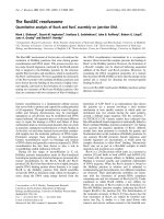
is better than the rest of values of n. Apart from this, a pictorial representation
of Product Fill Rate (PFR) using equation (6) for all three allocation models has
been given in Figure 1. For LA, PFR ranges from 50% to 100%, whereas it is
44% to 100% for UA, and 62% to 100% for IPA. Though LA favors high demand
retailers, yet it is giving 100% PFR for just one retailer. But in case of UA and
IPA, more than 50% of retailers are getting 100% PFR . Even IPA is better than

424

K., Chandra Jaggi, et al. / Quantitative Analysis for Measuring

UA as it not only satisfies higher percentage of retailers, but also it gives higher
range of PFR.
Now, one can think that whether inflating or deflating orders affect the individual
profits of the retailers. To study this, we did an analysis where the retailer”s demands were slightly changed,hence, their relative positions got changed,too.

Figure 1: Product Fill Rate

Table 7: % change in profits of IPA w.r.t different ‘n’ of Uniform Allocation Model
Retailer n=4
n=5
n=6
n=7
n=8
n=9
n=10
R1
7.64
15.28
15.28
22.91
30.55
38.19
45.83
R2
0.00

7.17
7.17
14.33
14.33
7.17
0.00
R3
0.00 -14.10 -14.10 -28.20 -35.14 -35.14 -35.14
R4
-6.62 -6.62
-6.62
-6.62
-6.62
-6.62
-6.62
R5
0.00
0.00
0.00
0.00
0.00
0.00
0.00
R6
0.00
0.00
0.00
0.00
0.00
0.00

0.00
R7
0.00
0.00
0.00
0.00
0.00
0.00
0.00
R8
0.00
0.00
0.00
0.00
0.00
0.00
0.00
R9
0.00
0.00
0.00
0.00
0.00
0.00
0.00
R10
0.00
0.00
0.00
0.00

0.00
0.00
0.00
Sum
1.02
1.73
1.73
2.43
3.02
3.49
3.96


K., Chandra Jaggi, et al. / Quantitative Analysis for Measuring

425

Example 2. A new set of retailer’s demand (Mi) for 10 retailers is given in
Table 8.
Table 8: Comparative Analysis between IPA, LA and UA.
Retailer Mi IPA
LA(‘n’=10)
UA(‘n’=4)
After Reallocation After Reallocation
R1
26
21
26
20
R2

25
20
25
20
R3
22
20
22
20
R4
21
20
20
21
R5
18
18
16
18
R6
15
15
13
15
R7
12
12
10
12
R8

10
10
8
10
R9
8
8
6
8
R10
6
6
4
6
Sum
163 150
150
150
In example 1, through Table 6 and Table 7, we have shown that for Linear Allocation, n=10 and for Uniform Allocation, n=4 is better than other values of ‘n’.
Hence, in Table 8 the comparison is shown corresponding to best of LA and UA.
It is evident that IPA is better than both allocation mechanisms and provides the
remedy to their major drawback, that is reallocation and to decide for how many
retailers demand must be satisfied completely (to evaluate the decision variable
‘n’). As the allocation mechanism is already declared by the supplier, therefore in
case of IPA, every retailer, who is ordering less than his proportionate share, will
get his demand satisfied. Those who are ordering more or inflating their demand
to get the allocation close to their original demand, may not be able to get their
demand satisfied fully. The retailers would be most benefited by truth inducing
mechanism rather than manipulable mechanism (MMi). It can further be proved
by inducing manipulation in Example 2. Let us suppose that R4 has manipulated

his demand to get more quantity .He demands for 23 units instead of 21 units.
Table 9 highlights the changes in comparison of other two algorithms.
Table 9 explains clearly that if any retailer manipulates his demand because
of declared allocation mechanism of supplier, he may get that increased demand
because of change of relative position, as happened with R4 . His actual demand
was 21, but according to LA, he gets 20. As a result, he inflated his demand to 23.
In this case he is getting 22 i.e. 1 unit more than his requirement. Whereas in case
of IPA, R4 is getting the same amount as he was getting in case of true demand.
This example shows that IPA supports truth-inducing mechanism.Similar type of
comparison is done between IPA and UA through Table 9.


426

K., Chandra Jaggi, et al. / Quantitative Analysis for Measuring

Table 9:
Retailer
R1
R2
R4
R3
R5
R6
R7
R8
R9
R10
Sum

Comparison between IPA,UA and LA
MMi IPA UA(’n’=4) LA(‘n’=10)
26
21
20
26
25
20
20
25
23
20
20
22
22
20
21
20
18
18
18
16
15
15
15
13
12
12
12
10

10
10
10
8
8
8
8
6
6
6
6
4
165
150
150
150

Consider that some retailer deflates his demand to get better level of satisfaction, say R2 deflates his demand from 25 units to 21 units. Now, when he had
given his true demand, i.e. 25 units, he was getting 20 units, which means he had
to bear the shortages of 5 units(as explained in Table 8), but after manipulation he
is getting 21 units, i.e. he is short of 4 units only. It means that manipulation can
favor him whereas in case of IPA, R2 is getting the same share as he was getting
before manipulation. Hence, neither inflation nor deflation is helpful in case of
IPA. Therefore, the best policy is to follow the Truth-Inducing-Mechanism, which
will help in reducing bullwhip effect.
In Example 1 and Example 2, all retailers have the same parameters,so the total profit of all retailers would remain the same,i.e. $4700, though the distribution
of profit among the retailers would change. To explore the situation further, one
more example is presented where retailers have different values of parameters like
selling price, shortage cost, and holding cost.
Example 3. The demand (Mi ) for 15 retailers along with their selling prices,

shortage cost, and holding cost are given in Table 10. Rest of the parameters are:
Cr =$50, C =750 units, cs =$30.
The allocation and profits corresponding to existing allocation models, i.e, LA
& UA are exhibited in Tables 11 & 12 and Tables 13 & 14, respectively. In both
allocation techniques, i.e. LA and UA, ’n’ is a decision variable and profit for
each value of ’n’ has to be calculated, whereas the proposed algorithm, IPA is
independent of ’n’, which is shown in Table 15.


K., Chandra Jaggi, et al. / Quantitative Analysis for Measuring

Retailer
R1
R2
R3
R4
R5
R6
R7
R8
R9
R10
R11
R12
R13
R14
R15

Table 10: Data for example 3
Demand Selling Price Holding cost

Mi
Pi
hi
140
60
1
130
60
1
120
60
1
115
61
0.85
110
61
0.85
105
62
0.75
100
62
0.75
98
63
0.65
95
63
0.65

92
64
0.6
85
64
0.6
78
65
0.55
70
66
0.55
65
66
0.55
65
67
0.5

427

shortage cost
Si
1.5
1.5
1.5
1.35
1.35
1.25
1.25

1.15
1.15
1.1
1.1
1.05
1.05
1.05
1

It is clearly visible from Table 11 that Linear allocation is giving zero allocation to
least demand retailer , which is not the case with Uniform and IPA. Corresponding
results for IPA are expressed in Table 15.


428

K., Chandra Jaggi, et al. / Quantitative Analysis for Measuring

Table 11: Demand AllocationRetailer
R1
R2
R3
R4
R5
R6
R7
R8
R9
R10
R11

R12
R13
R14
R15
SUM

Demand
Mi
140
120
110
100
95
85
70
65
55
48
42
30
22
20
18
1020

n=7
140
120
110
100

95
85
70
30
0
0
0
0
0
0
0
750

n=8
140
115
105
95
90
80
65
60
0
0
0
0
0
0
0
750

n=9
130
110
100
90
85
75
60
55
45
0
0
0
0
0
0
750

Allocation Ai
n=10 n=11 n=12
128
130
128
106
103
102
96
93
92

86
83
82
81
78
77
71
68
67
56
53
52
51
48
47
41
38
37
34
31
30
07
25
24
0
0
12
0
0
0

0
0
0
0
0
0
750
750
750

Table 12: Profits for Retailers Retailer
R1
R2
R3
R4
R5
R6
R7
R8
R9
R10
R11
R12
R13
R14
R15
Sum

n=7
1260

1080
990
1015
964.25
956.25
787.5
330.25
-63.25
-52.8
-46.2
-31.5
-23.1
-21
-18
7127.4

n=8
1260
1027.5
937.5
957.5
906.75
893.75
725
735.25
-63.25
-52.8
-46.2
-31.5
-23.1

-21
-18
7187.4

n=9
1155
975
885
900
849.25
831.25
662.5
667.75
544.25
-52.8
-46.2
-31.5
-23.1
-21
-18
7277.4

Linear Allocation

n=10
1134
933
843
854
803.25

781.25
612.5
613.75
490.25
440.2
-46.2
-31.5
-23.1
-21
-18
7365.4

n=13
124
102
92
82
77
67
52
47
37
30
24
12
4
0
0
750

n=14
122
102
92
82
77
67
52
47
37
30
24
12
4
2
0
750

n=15
122
102
92
82
77
67
52
47
37
30
24

12
4
2
0
750

Linear Allocation

Profits
n=11
1155
901.5
811.5
819.5
768.75
743.75
575
573.25
449.75
396.7
316.3
-31.5
-23.1
-21
-18
7417.4

n=12
1134
891

801
808
757.25
731.25
562.5
559.75
436.25
382.2
301.8
154.5
-23.1
-21
-18
7457.4

n=13
1092
891
801
808
757.25
731.25
562.5
559.75
436.25
382.2
301.8
154.5
42.9
-21

-18
7481.4

n=14
1071
891
801
808
757.25
731.25
562.5
559.75
436.25
382.2
301.8
154.5
42.9
12
-18
7493.4

n=15
1071
891
801
808
757.25
731.25
562.5
559.75

436.25
382.2
301.8
154.5
42.9
12
-18
7493.4


429

K., Chandra Jaggi, et al. / Quantitative Analysis for Measuring

Table 13: Demand AllocationRetailer
R1
R2
R3
R4
R5
R6
R7
R8
R9
R10
R11
R12
R13
R14
R15

SUM

Demand
Mi
140
120
110
100
95
85
70
65
55
48
42
30
22
20
18
1020

n=7
64
64
64
64
64
64
66
65

55
48
42
30
22
20
18
750

n=8
64
64
64
64
64
64
66
65
55
48
42
30
22
20
18
750

n=9
63
63

63
63
63
65
70
65
55
48
42
30
22
20
18
750

Uniform Allocation

Allocation Ai
n=10 n=11 n=12
61
60
57
61
60
57
61
60
57
61
60

57
61
60
67
75
80
85
70
70
70
65
65
65
55
55
55
48
48
48
42
42
42
30
30
30
22
22
22
20
20

20
18
18
18
750
750
750

n=13
57
57
57
57
67
85
70
65
55
48
42
30
22
20
18
750

n=14
52
52
52

52
87
85
70
65
55
48
42
30
22
20
18
750

n=15
50
50
50
50
95
85
70
65
55
48
42
30
22
20
18

750


430

K., Chandra Jaggi, et al. / Quantitative Analysis for Measuring

Table 14: Profit for retailersRetailer
R1
R2
R3
R4
R5
R6
R7
R8
R9
R10
R11
R12
R13
R14
R15
Sum

n=7
462
492
507
601

607.75
693.75
737.5
802.75
679.25
643.2
562.8
433.5
339.9
309
297
8168.4

n=8
462
492
507
601
607.75
693.75
737.5
802.75
679.25
643.2
562.8
433.5
339.9
309
297
8168.4

n=9
451.5
481.5
496.5
589.5
596.25
706.25
787.5
802.75
679.25
643.2
562.8
433.5
339.9
309
297
8176.4

n=10
430.5
460.5
475.5
566.5
573.25
831.25
787.5
802.75
679.25
643.2

562.8
433.5
339.9
309
297
8192.4

Uniform Allocation
Profits
n=11
420
450
465
555
561.75
893.75
787.5
802.75
679.25
643.2
562.8
433.5
339.9
309
297
8200.4

n=12
388.5
418.5

433.5
520.5
642.25
956.25
787.5
802.75
679.25
643.2
562.8
433.5
339.9
309
297
8214.4

Table 15: Allocation and Profit for retailersRetailer
R1
R2
R3
R4
R5
R6
R7
R8
R9
R10
R11
R12
R13
R14

R15
Sum

Demand
140
120
110
100
95
85
70
65
55
48
42
30
22
20
18
1020

Allocation
65
65
65
64
64
64
64
64

55
48
42
30
22
20
18
750

n=13
388.5
418.5
433.5
520.5
642.25
956.25
787.5
802.75
679.25
643.2
562.8
433.5
339.9
309
297
8214.4

n=14
336
366

381
463
872.25
956.25
787.5
802.75
679.25
643.2
562.8
433.5
339.9
309
297
8229.4

n=15
315
345
360
440
964.25
956.25
787.5
802.75
679.25
643.2
562.8
433.5
339.9
309

297
8235.4

IPA

Profits
472.5
502.5
517.5
601
607.75
693.75
712.5
789.25
679.25
643.2
562.8
433.5
339.9
309
297
8161.4

Table 16 depicts the percentage change in profits of various retailers due to
IPA with respect to different values of ‘n’ of LA . Respective values for UA are
expressed in Table 17.Table 12, Table 14 and Table 15 infer that in case of different
parameters total profit for UA is little higher as compared to IPA, but PFR is
low, which is explained in Figure 2. It shows that customer satisfaction rate is

431

K., Chandra Jaggi, et al. / Quantitative Analysis for Measuring

low in UA. Moreover the appearing high profit may be false information because
of manipulable mechanism.
Table 16: % change in profits of IPA w.r.t different ‘n’ of Linear Allocation
Retailer
R1
R2
R3
R4
R5
R6
R7
R8
R9
R10
R11
R12
R13
R14
R15
Sum

n=7
-166.7
-114.9
-91.3
-68.9

-58.7
-37.8
-10.5
58.2
109.3
108.2
108.2
107.3
106.8
106.8
106.1
262.0

n=8
-166.7
-104.5
-81.2
-59.3
-49.2
-28.8
-1.8
6.8
109.3
108.2
108.2
107.3
106.8
106.8
106.1
268.1

n=9
-144.4
-94.0
-71.0
-49.8
-39.7
-19.8
7.0
15.4
19.9
108.2
108.2
107.3
106.8
106.8
106.1
266.8

% change in Profits
n=10
n=11
n=12
-140.0 -144.4 -140.0
-85.7
-79.4
-77.3
-62.9
-56.8
-54.8

-42.1
-36.4
-34.4
-32.2
-26.5
-24.6
-12.6
-7.2
-5.4
14.0
19.3
21.1
22.2
27.4
29.1
27.8
33.8
35.8
31.6
38.3
40.6
108.2
43.8
46.4
107.3
107.3
64.4
106.8
106.8
106.8

106.8
106.8
106.8
106.1
106.1
106.1
255.3
238.8
220.3

n=13
-131.1
-77.3
-54.8
-34.4
-24.6
-5.4
21.1
29.1
35.8
40.6
46.4
64.4
87.4
106.8
106.1
209.8

n=14
-126.7

-77.3
-54.8
-34.4
-24.6
-5.4
21.1
29.1
35.8
40.6
46.4
64.4
87.4
96.1
106.1
203.6

n=15
-126.7
-77.3
-54.8
-34.4
-24.6
-5.4
21.1
29.1
35.8
40.6
46.4
64.4
87.4

96.1
106.1
203.6

Table 17: % change in profits of IPA w.r.t different ‘n’ of Uniform Allocation
Retailer
R1
R2
R3
R4
R5
R6
R7
R8
R9
R10
R11
R12
R13
R14
R15
Sum

n=7
2.2
2.1
2.0
0.0
0.0
0.0

-3.5
-1.7
0.0
0.0
0.0
0.0
0.0
0.0
0.0
1.1

n=8
2.2
2.1
2.0
0.0
0.0
0.0
-3.5
-1.7
0.0
0.0
0.0
0.0
0.0
0.0
0.0
1.1

n=9

4.4
4.2
4.1
1.9
1.9
-1.8
-10.5
-1.7
0.0
0.0
0.0
0.0
0.0
0.0
0.0
2.4

% change in
n=10 n=11
8.9
11.1
8.4
10.4
8.1
10.1
5.7
7.7
5.7
7.6
-19.8

-28.8
-10.5
-10.5
-1.7
-1.7
0.0
0.0
0.0
0.0
0.0
0.0
0.0
0.0
0.0
0.0
0.0
0.0
0.0
0.0
4.7
5.9

Profits
n=12
17.8
16.7
16.2
13.4
-5.7
-37.8

-10.5
-1.7
0.0
0.0
0.0
0.0
0.0
0.0
0.0
8.4

n=13
17.8
16.7
16.2
13.4
-5.7
-37.8
-10.5
-1.7
0.0
0.0
0.0
0.0
0.0
0.0
0.0
8.4

n=14

28.9
27.2
26.4
23.0
-43.5
-37.8
-10.5
-1.7
0.0
0.0
0.0
0.0
0.0
0.0
0.0
11.8

n=15
33.3
31.3
30.4
26.8
-58.7
-37.8
-10.5
-1.7
0.0
0.0
0.0
0.0

0.0
0.0
0.0
13.2

Now, through Table 16 and Table 17 , it is evident that total % change in
profits is positive for IPA as compared to LA and UA irrespective of value of n.


432

K., Chandra Jaggi, et al. / Quantitative Analysis for Measuring

This analysis shows that though the profit for IPA seems to be little lesser than
UA, but it might not be a real situation. The reason for this claim is that LA
and UA are giving manipulated information in market. For getting better share in
monopolistic environment, they are generating false demand, so the corresponding
profit is also false. Whereas IPA is promoting only truth inducing mechanism, so
whatever profit appears is achievable. Moreover IPA is providing much better
PFR, which can be seen in figure 2.

Figure 2: Product Fill Rate

Through above analysis we have shown that IPA is better than two existing algorithms in literature.
6. CONCLUSIONS and SUGGESTIONS
Present paper introduces an allocation algorithm for rationing of limited capacity among retailers in order to measure and suppress bullwhip effect. The
proposed IPA algorithm , which is coded in C++, deals with two main bottlenecks of existing mechanism in literature i.e, LA and UA to take a decision for
number of customers who will get their demand satisfied with priority (n) and
to avoid reallocation. Further, it also promotes truth inducing mechanism, which
eventually suppresses bullwhip effect. Through a numerical example, it has been

established that IPA promotes truth inducing mechanism, which suggests that a
retailer should reveal his actual demand without making any manipulation. Finally, a comparative analysis is presented between IPA,and LA and UA considering
profits and product fill rate.


K., Chandra Jaggi, et al. / Quantitative Analysis for Measuring

433

Acknowledgement: We would like to express our sincerest thanks to the
Editor and anonymous reviewers for their constructive and valuable comments in
improving the manuscript.

REFERENCES
[1] Cachon,G.P.& Lariviere, M.A. “Capacity choice and allocation: Strategic behavior and
supply chain performance”, Management Science, 45 (8) (1999)1091–1108.
[2] Cachon,G.P.& Lariviere, M.A., “An equilibrium analysis of linear and proportional allocation of scarce capacity”, IIE Transactions, 31 (9) (1999) 835–849.
[3] Cachon,G.P.,Randall,T.& Schmidt,G.M , “In search of the bullwhip effect”, Manufacturing& Service Operations Management, 9 (4) (2007) 457- 479.
[4] Chatfield,D.C.& Pritchard, A.M., “Returns and the bullwhip effect”, Transportation Research Part E, 49 (2013) 159 -175.
[5] Chen,L.,& Lee,H.L., “Bullwhip effect measurement and its implications”, Operations Research, 60 (2012) 771-784.
[6] Chopra, S., and Meindl, P, Supply Chain management: Strategy, planning and operation,
Upper Saddle River, Pearson Prentice Hall, New Jersey, 2001.
[7] Dai,j., Peng S.,& Li,S., “Mitigation of Bullwhip Effect in Supply Chain Inventory Management Model”, Procedia Engineering 174 (2017) 1229 - 1234.
[8] Dejonckheere,J.,Disney,S.M.,Lambrecht,M.R.,& Towill,D.R., “Measuring and avoiding the
bullwhip effect : a control theoretic approach”, European Journal of Operational Research,
147 (3) (2003) 567590.
[9] Deshpande V, Schwarz L B , “Optimal capacity choice and allocation in decentralized
supply chains”, Working paper, Krannert School of Management, Purdue University, West
Lafayette, Indiana, USA, 2002.
[10] Forrester, J.W. , Industrial Dynamics, Cambridge M.A., MIT Press, Cambridge, 1961.

[11] Jaggi, C.K., Aggarwal, K.K., And Verma,M. , “Allocation Game in a single period Supply
Chain Model”, Revista Investigacion Operacional, 31 (3) (2010) 258–267.
[12] Kaplan, A , “Stock Rationing”, IIE Management Science, 15 (5) (1969) 260–267.
[13] Lee, H., Padmanabhan, P and Whang, S. , “The Bullwhip effect in supply chains”, Sloan
management review, 38 (1997 (a)).
[14] Lee, H., Padmanabhan, P and Whang, S., “Information distortion in a supply chain: The
bullwhip effect”, Management Science, 43 (1997 (b)) 546–558.
[15] Nahmias, s.And Demmy, W.S., “Operating Characteristics of an inventory system with
Rationing”, Management Science, 27 (11) (1981) 1236–1245.
[16] Nemtajela,N. & Mbohwa,C., “Relationship between inventory management and uncertain
demand for fast moving consumer goods organisations”, 14th Global Conference on Sustainable Manufacturing, GCSM 3-5 October 2016, Stellenbosch, South Africa, 2016.
[17] Ravi Ravindran A , “Multiple Criteria Decision Making in Supply Chain Management”,
CRC press, Taylor and Francis Group.