Modification of topsis method for solving of multicriteria tasks
Bạn đang xem bản rút gọn của tài liệu. Xem và tải ngay bản đầy đủ của tài liệu tại đây (351.88 KB, 27 trang )
Yugoslav Journal of Operations Research
Volume 20 (2010), Number 1, 117-143
10.2298/YJOR1001117M
MODIFICATION OF TOPSIS METHOD FOR SOLVING OF
MULTICRITERIA TASKS
Zoran MARKOVIĆ
PE PTT Communications "Serbia"
Received: March 2005 / Accepted: February 2010
Abstract: This paper describes the possible modifications of one of the multi-criteria
analysis methods that possess certain advantages in cases of solving the real business
problems. We will discuss the TOPSYS method, whereas the modification reflects in
change of the determination manner of the ideal and anti-ideal points in criteria
environment, in standardization of quantification and fuzzycation of the attributes in
cases of criteria expressed by linguistic variables.
Keywords: Decision-making, multi-criteria analyses, attributes, fuzzy attribute description.
1. INTRODUCTION
Modern operational methods in large hierarchy-structured business systems
imply making numerous important business decisions in a short period of time, which
means that managers are often forced to use specific tools in order to be able to make
minimum risk in quality decisions. It could be said that the last quarter of the 20th century
and the beginning of new millennium have flourished in various studies and researches
aiming to develop the decision-making mechanisms and methods in situations in which
relationships within the system and the environment are becoming ever more
complicated and more dynamic and when the reaction time to actual or assumed
dysfunctions becomes a considerable factor of success. The majority of business
decisions are made in conflict or partially conflict criteria situations, in which cases the
uni-criterion tasks' solving methods are almost inapplicable. Practice has imposed the
development of new methods which have acknowledged the conflict quality of criteria or
goals. This resulted in development of multi-criteria and multi-target methods of real
problems' solving. Taxonomy of the multi-criteria tasks' solving method is shown bellow
in the Picture 1. [5] [2].
118
Z., Marković / The Topsis Method Modification
This paper describes the TOPSYS method of solving the multi-criteria decisionchoosing tasks that implies full and complete information on criteria, expressed in
numerical form. The method is very useful for solving of real problems; it provides us
with the optimal solution or the alternative's ranking. In addition to this, it is not so
complicated for the managers as some other methods which demand additional
knowledge. TOPSYS method would search among the given alternatives and find the one
that would be closest to the ideal solution but farthest from the anti-ideal solution at the
same time. The essence of it reflects in determination of the Euclidean distances from the
alternatives (represented by points in n-dimensional criteria space) to the ideal and antiideal points. Modification of the method aims to set a different manner of determining
the ideal and anti-ideal point – through standardization of linguistic attributes'
quantification and introduction of fuzzy numbers in description of the attributes for the
criteria expresses by linguistic variables.
INFORMATION TYPE
IMPORTANT
BASIC METHOD OF DECISION MAKER INFORMATION CLASSES
CHARACTERISTICS
- DOMINATION
- MAXMIN
- MAXIMAX
1WITHOUT
INFORMATION
2.1. STANDARD
LEVEL
MCD
2. INFORMATION
ABOUT
ATTRIBUTE
2.2. ORDINAL
2.3. MAIN
(CARDINAL)
2.4MARGINAL
RATIO OF CHANGE
3. INFORMATION
ABOUT ACTION
3.1. "PAIRED"
PREFERENCES
3.2. ORDER OF PAIRED
VICINITIES
-CONJUNCTIVE METHOD
DISJUNCTIVE METHOD
LEXICOGRAPHIC
-ELIMINATION BY ASPECTS
-PERMUTATIONS METHOD
-METHOD OF LINEAR AWARDING
-METHOD OF SIMPLE ADITIVE
GRAVITIES
-METHOD OF HIERARCHICALLY
ADITIVE GRAVITIES
- ELECTRE
- TOPSIS
-HIERARCHICAL
REPLACEMENT
-LINMAP
-INTERACTIVE METHOD
-MULTIDIMENSIONAL
RANKING WITH IDEAL POINT
Picture 1 Taxometry of multi-criteria decision-making method (MCD)
2. SETTING OF PROBLEMS AND TOPSYS METHOD
In cases where real problems are to be solved, the managers often have to make
a decision by choosing one out of many alternative solutions based on several decisionmaking criteria of opposite or partially opposite characteristics. Therefore, let us assume
that we are given m – alternatives and that n-criteria is being assigned to each of them,
Z., Marković / The Topsis Method Modification
meaning that we are choosing the most acceptable alternative
alternative group, taking into account all criteria simultaneously.
119
a * out of the final A
A = [a1 , a2 ,..., am ]
Each alternative ai ; i = 1,2,..., m is described by attribute values f j ; j = 1,2,..., n
marked as follows: xij ; i = 1, m; j = 1, n . Criteria f j may be of profit (benefit) or
expenditure (cost) type.[1] Profit type criteria means that greater value of attribute is
preferred to lesser attribute value (herein represented by "max"), while cost type criteria
means that lesser attribute value is preferred to greater value of attribute (herein
represented by "min").
The above may be illustrated with the following matrix O:
f1
f2
L
fj
L
fn
a1
x11
x12
L
x1 j
L
x1n
a2
x21
x22
L
x2 j
L
x2 n
M
ai
M
xi1
M
xi 2
M
L
M
xij
M
L
M
xin
M
M
M
M
M
M
M
am
xm1
xm 2
L
xmj
L
xmn
⎛ max ⎞ ⎛ max ⎞
⎜
⎟ ⎜
⎟
⎝ min ⎠ ⎝ min ⎠
⎛ max ⎞
⎜
⎟
⎝ min ⎠
⎛ max ⎞
⎜
⎟
⎝ min ⎠
The elements of the matrix O are real numbers (not negative) or linguistic
expressions from the given group of expressions. Linguistic attributes have to be
quantified within previously determined and agreed value scale. The most commonly
used scales are as follows:
Ordinal scale
Interval scale
Relationship scale
Ordinal scale determines the ranking of actions, whereas the relative distances
between the ranks are not taken into account, unlike the Interval scale where equal
differences between the attribute values and defined benchmarks are determined. Ratio
scale also ensures equal relations between the attribute values but the benchmarks are not
defined beforehand. The author’s opinion is that Interval scale represents the suitable tool
to be used when performing quantification of qualitative attributes. The most commonly
used scale is 1 to 9, since the extremes of the attributes for the criteria being analyzed are
120
Z., Marković / The Topsis Method Modification
usually unknown. The table bellow shows one of the methods of translating the
qualitative attributes into quantitative attributes.
Qualitative
estimation
Quantitative
estimation
bad
good
avarage
1
9
3
7
5
5
very
good
7
3
excellent
Type of
criteria
Max
min
9
1
Quantification of qualitative criteria can be performed in many different ways.
One of them is so called fuzzycation, which gives account of the ambiguities occurring at
expression of linguistic variables. Therefore, the matrix O becomes quantified according
to each criterion and as such, this matrix is called – quantified decision-making matrix
O1.
In order for the task to be solved it is necessary to normalize the attribute values,
i.e. to perform the “unification” or “make the attributes non-dimensional”, which means
that the attribute values would be set within 0 – 1 interval. Normalization of the
quantified matrix O1 can be performed in two ways, as follows:
1.
2.
Vectorial normalization, and
Linear normalization.
In vectorial normalization procedure each element of quantified decisionmaking matrix is divided by its own norm. The norm represents the square root of the
addition of element value squares, according to each criterion. The procedure is as
follows: [6]
The norm is calculated for each j-column of decision-making matrix:
m
j=
norma
∑
x
2
ij
; ( j = 1 ,..., n
)
i=1
Whereas xij - represents the value of j-attribute for i-alternative.
rij represents the elements of new, normalized decision-making matrix R, and
are calculated in the following manner:
For the max type criteria,
r ij =
x ij
norma
; ( i = 1 , 2 ,..., m ) ( j = 1 , 2 ,..., n
)
j
For the min type criteria,
r ij = 1 −
x ij
norma
; ( i = 1 , 2 ,..., m ) ( j = 1 , 2 ,..., n
)
j
Depending on the criteria type, linear normalization of attributes is performed in
a way in which attribute value is divided by maximum attribute value for given max type
Z., Marković / The Topsis Method Modification
121
criteria, i.e. by supplementing - up to1 - for given min type criteria. This results in linear
decision-making matrix R with the following elements:
For the max type criteria:
r ij =
x ij
x
*
j
⎧
; x *j = ⎨ x
⎩
max
j
x ij ⎫⎪
⎬ ; i = 1, m ; j = 1, n
i
⎪⎭
For min type criteria:
r ij = 1 −
x ij
x
*
j
⎧
; x *j = ⎨ x
⎩
max
j
x ij ⎫⎪
⎬ ; i = 1, m ; j = 1, n
i
⎪⎭
Nevertheless, in order to preserve the maximum initial information in the course
or further action in relation to initial attribute values and attribute values of other criteria,
for the min type criteria, it is necessary to perform more precise copying of attribute
values into the 0 -1 interval. Namely, normalized attribute values for max type criteria
would be in the interval p-1, and 0 p p p 1 , while in case of min type criteria that value
belongs in the interval from 0-p, and 0 p p p 1 . From these grounds we suggest the
linear normalization with copying, as in max type criteria, meaning that:
rij = 1 −
x ij − x −j
x *j
⎧
; x *j = ⎨ x
⎩
j
⎧⎪
max x ij ⎪⎫ −
min x ij ⎫⎪
⎬; x j = ⎨ x j
⎬ ; i = 1, m ; j = 1, n
i
i
⎪⎭
⎪⎩
⎪⎭
After the normalized decision-making matrix is made, it is necessary to
determine the coefficients of relative criteria importance w j ; j = 1,2,..., n - which are also
n
being normalized, which results in the following: ∑ w j = 1
j =1
Relative importance of criteria represents a significant part of multi-criteria task
set-up, since it ensures the relation between criteria which, by the rule, are not of the
same value. Relative importance of criteria depends on subjective estimation of the DM
(Decision Maker) and has a significant influence on the final result. Multiplication of
each normalized matrix’s element rij with the assigned weight coefficient w j results in
decision-making matrix V where one of the multi-criteria tasks’ solving methods is
applied.
The
elements
of
decision-making
matrix
are
as
follows:
v ij = w j r ij ; i = 1 , 2 ,..., m ; j = 1 , 2 ,..., n
Selection of multi-criteria tasks’ solving method depends on complexity of the
task as well as on the preferred result (rank alternative, the best alternative, group of
satisfactory alternatives, etc.)
In the text which follows we shall discuss the TOPSYS method resulting in rank
alternative, being the best alternative at the same time, taking into consideration all
criteria simultaneously.
122
Z., Marković / The Topsis Method Modification
TOPSYS – (Technique for Order Preference by Similarity to Ideal Solution) [5]
method, determines the similarity to ideal solution. Therefore, it introduces the criteria
space in which every alternative Ai is represented by a point in the n-dimensional criteria
space and coordinates of those points are attribute values of decision-making matrix V.
Next step is determining of ideal and anti-ideal points and finding the alternative with the
closest Euclidean distance from the ideal point, but at the same time, the farthest
Euclidean distance from the anti-ideal point. Picture 2 represents the example of twodimensional criteria space in which every alternative Ai possesses the coordinates which
are equal to normalized values of the assigned attributes multiplied by normalized weight
coefficients, coordinates of ideal A* and anti-ideal point A − , as well as the Euclidean
alternative distances from the ideal and anti-ideal point.
Figure 2 Euclidean alternative distances from the ideal and anti-ideal point.
TOPSYS method builds on the assumption that mxn decision-making matrix O
includes m-alternatives and n-criteria:
a1
a2
O= M
ai
M
am
f1
x11
x21
M
xi1
M
xm1
f2
x12
x 22
M
xi 2
M
xm 2
⎛ max ⎞
⎜⎜
⎟⎟
⎝ min ⎠
⎛ max ⎞
⎜⎜
⎟⎟
⎝ min ⎠
L fj
L x1 j
L x2 j
M
M
L xij
M
M
L xmj
L fn
L x1n
L x2 n
M
M
L xin
M
M
L xmn
⎛ max ⎞
⎜⎜
⎟⎟
⎝ min ⎠
⎛ max ⎞
⎜⎜
⎟⎟
⎝ min ⎠
ai - i_ alternative ; xij - attribute value i_alternative for j_ criteria
Z., Marković / The Topsis Method Modification
123
It is also assumed that attributes expressed by linguistic terms have been
quantified, as well as that benefits of each individual criterion have been determined and
that relative criteria weights w j have also been defined. Further procedure can be
described in 6 steps, as follows:
1. First step – calculating the normalized matrix using the vector normalization,
whereas the matrix elements for the max type criteria are:
x ij
r ij =
(j
m
∑
x
2
= 1 ,.... n
)
ij
i =1
and for the min type criteria:
x ij
r ij = 1 −
(j
m
∑
x
2
= 1 ,.... n
)
ij
i=1
This results in normalized decision-making matrix as shown bellow:
f1
f2
a1
r11
r12
a2
r21
r22
M
ai
M
am
M
ri1
M
rm1
M
ri 2
M
rm 2
⎛ max ⎞ ⎛ max ⎞
⎜⎜ min ⎟⎟ ⎜⎜ min ⎟⎟
⎝
⎠ ⎝
⎠
L
L
L
M
L
M
L
fj
r1 j
r2 j
M
rij
M
rmj
⎛ max ⎞
⎜⎜ min ⎟⎟
⎝
⎠
L
L
L
M
L
M
L
fn
r1n
r2 n
M
rin
M
rmn
⎛ max ⎞
⎜⎜ min ⎟⎟
⎝
⎠
2. Second step – multiplication of normalized matrix elements with normalized
n
weight coefficients w j ; j = 1,2,..., n such as that: ∑ w j = 1 whereas the elements of the
j =1
modified decision-making matrix are: vij = w j rij
3. Third step – determining the ideal and anti-ideal points in n-dimensional
criteria space, so that ideal point is as follows:
124
Z., Marković / The Topsis Method Modification
A* = (
max
i
j ∈ J ), (
v ij
min
i
v ij
j ∈ J ' ) i = 1,2,..., m
A* = (v1* , v 2* ,..., v *j ,..., v n* ) - Ideal alternative coordinates;
A− = (
min
i
j ∈ J ), (
vij
max
i
vij
j ∈ J ' ) i = 1,2,..., m
A − = (v1− , v 2− ,..., v −j ,..., v n− ) - Anti-ideal alternative coordinates;
Whereas J ⊂ {1,2,..., n) j −max} applies for the max type criteria,
while J ' ⊂ {1,2,..., n) j − min} applies for the min type criteria.
In this way, the coordinates of the ideal A* and anti-ideal point A − in the ndimensional criteria space have been determined.
4. Fourth step – calculating of Euclidean distance S i* of each alternative a i ,
from the ideal point and S i− of each alternative a i from the anti-ideal point A − .
S i* =
n
* 2
∑ (v ij − v j ) , i = 1,..., m - Euclidean distance of the iⁿ alternative from
j =1
the ideal point;
S i− =
n
− 2
∑ (v ij − v j ) , i = 1,..., m - Euclidean distance of the iⁿ alternative from
j =1
the anti-ideal point.
5. Fifth step – calculating the relative similarity of the alternatives from the ideal
and anti-ideal points which is done in the following manner:
Ci =
S i−
S i* + S i−
If Ci =1 then
that
;0 p Ci ≤ 1; i = 1,..., n
a i = A* and if Ci =0, then a i = A − . Therefore, the conclusion is
ai is closer to A* if the Ci is closer to value 1.
6. Sixth step – setting up the rank according to Ci , meaning that the bigger Ci
is - the better the alternative would be.
3. MODIFICATION OF TOPSYS METHOD
The author is familiar with two modifications of TOPSYS method, whereas the
first one aims to simplify the procedure of best action selection, while the other one deals
with fuzzycation of attributes. First modification was performed by Yoon and Hwang [5]
by using the simple additive weight method as the base. Modification reflects in the fact
Z., Marković / The Topsis Method Modification
125
that relative closeness is not determined on the basis of the Euclidean distance but it is
based on the city distance; therefore setting up the alternative rank according to the
shortest city distance to the ideal point but, at the same time, the longest distance from
the anti-ideal point. The basic TOPSYS method includes the exact numerical descriptions
of attributes, whereas the authors of the above said modification translate linguistic
descriptions into numerical forms within the determined value scale. In case the manager
is doubtful about the available subjective estimations, the method provides the option of
calculating the replacement margin by using the indifference curve. More detailed
description of this modification can be found under reference [5].
Another modification in relation to the attribute fuzzycation (as described in
detail under [3]), means that each attribute is described by a discrete fuzzy number. This
being done, we determine the relations of order between discrete fuzzy groups, as well as
the probabilities of belonging to a group and also the measures of inferiority of the
alternatives according to a certain criterion. The rank is established based on belief that
alternative is worse then ideal solution but better then anti-ideal solution. Modification is
in deed interesting, but the author is of the opinion that it is not necessary to carry out
fuzzycation of all criteria but only those which are being expressed by linguistic terms. In
addition to this, the proposed modification makes its practical application more difficult.
The author will try to solve the problem of noticed deficiencies of TOPSYS
method when applied in practice, through modification of basic method, as described in
the text which follows.
3. 1. Implementation of ideal and anti-ideal alternative
The author's opinion is that determining of ideal and anti-ideal points also
represents a deficiency of the original TOPSYS method, because in the original method,
maximum and minimum values of attributes according to all criteria represent the
coordinates of ideal and anti-ideal points. Nevertheless, the attribute values in specific
tasks are not always ideal for the given criterion. When solving the real problems
managers tend to define ideal and anti-ideal values for each criterion and compare the
attributes with the extremes defined in that manner. Potential solutions in most cases
deviate from the ideal, and therefore the task is to find the solution that would be closest
to the ideal, taking into account all criteria simultaneously. Qualitative criteria are
especially interesting when used to express evaluations of managers within some value
scale. If we consider the 1 to 10 value scale, the attribute values are often to be found
somewhere in between the extreme values and that is why in the original method,
maximum and minimum attribute values (rather then extreme scale values) are taken as
coordinates of the ideal and anti-ideal points. Therefore, the manager assumes that the
ideal value is equal to 10 and then assigns other attribute values in accordance to that
value, so it is logical to assign the value 10 for the attribute value of ideal alternative, i.e.
to assign the value 1 for the anti-ideal. When dealing with the criteria whose attributes
could be expressed in numerical terms, it is always questionable whether the maximum
and minimum attribute values are truly ideal and anti-ideal or it is up to the manager
himself to estimate if those values could be more extreme. This only adds to manager's
subjectivity during the task solving process, but on the other hand, it contributes to more
precise and clear definitions of the ideal and anti-ideal solutions which are later used as
benchmarks for all other alternatives. Attribute values for the ideal and anti-ideal
alternative must comply with the following requirement:
126
Z., Marković / The Topsis Method Modification
x + ≥ max
x
−
j
≤ min
( j = 1 ,.... n ), ( i = 1 ,... m )
x ij ( j = 1 ,.... n ), ( i = 1 ,... m )
x ij
This paper suggests modification of the basic method through introduction of
two new alternatives. One of the alternatives would possess the attributes of maximum
theoretical value (i.e. ideal) as opposed to the other alternative that would possess the
attributes of minimum theoretical value (i.e. anti-ideal). It goes without saying that when
determining the ideal and anti-ideal values we have to bear in mind the criteria benefits,
maintaining the possibility to translate the cost criteria into profit criteria by inversion of
attribute values. Thus the attributes of the said alternatives would serve as ideal and antiideal points' coordinates.
This can be demonstrated by a simple example involving only two criteria. Let
us assume that both criteria are of linguistic nature and that estimations are expressed in
the interval from 1 to 10. Let us also assume that we have four alternatives and that the
table bellow shows the decision-making matrix after the quantification process:
Alternative 1
Alternative 2
Alternative 3
Alternative 4
Weight coefficients
Criteria 1
9
3
4
9
0,4
Criteria 2
2
6
6
4
0,6
After we perform all calculations, we would come to alternatives' coordinates,
ideal and anti-ideal points, provided that calculation manner is a standard one and that
ideal and anti-ideal alternatives have been introduced. As both criteria are of linguistic
nature, let us assume they are of profit character coordinates of the ideal point are the
attribute values of the alternative 1 for the first criterion and alternative 3 for second
criterion, when standard manner is in question. Therefore, in case of standard calculation,
it means that the ideal characteristic of criterion 1 is of value 9, which is not logical if we
consider that evaluations are made within the value scale from 1 to 10. Also, the values
of anti-ideal point coordinates are being changed in the identical manner. Introduction of
additional alternatives resulted in change of criteria space as well as in alternatives’
coordinates. Consequently, the change also occurred in Euclidean distances from the
ideal and anti-ideal points, which may not necessarily influence the alternative ranking.
Standard way of calculation
Ideal point
0,26326
0,37533
Alternative 1
0,26326
0,12511
Alternative 2
0,08775
0,37533
Alternative 3
0,117
0,37533
Alternative 4
0,26326
0,25022
Anti ideal point
0,08775
0,12511
Modified way of
0,2357
0,43189
0,21213
0,08638
0,07071
0,25913
0,09428
0,25913
0,21213
0,17276
0,02357
0,04319
Our example clearly shows that points within the criteria space have moved
towards the coordinate beginning, as shown in the Picture 3.
127
Z., Marković / The Topsis Method Modification
Now, if we add the relative closeness of the alternatives and ideal and anti-ideal
point we will come to the modified order of the alternatives as shown in the table bellow.
Standard method
Alternative 4
0,632726
Alternative 3
0,632689
Alternative 2
0,587747
Alternative 1
0,412253
Modified method
Alternative 3
0,504404
Alternative 2
0,480587
Alternative 4
0,467875
Alternative1
0,358391
Kr1
A1
0,26326
A1
0,2357
I+
A4
I+
A3
0,08775
0,02378
A4
I0,03772
I-
A3
A2
A2
0,12511
0,37533
0,43189
Kr2
Figure 3 Points in criteria spaces for standard and modified calculation manner
When dealing with more complex tasks and when ideal and anti-ideal
alternatives are introduced, the ideal point is more distant from coordinate beginning in
comparison to the ideal point in standard method. Also, it is clearly shown that
coordinates of the alternatives are quite different when those two calculation manners are
applied, because the introduction of two additional alternatives results in change of
attributes in the process of data matrix normalization. If greater number of criteria and
alternatives are involved, that difference would diminish.
Same would happen in case of normalization performed through linear
attributes’ normalization, whereas the differences between normalized attribute values
would be greater in modified manner of calculation then in standard manner of
calculation. Bellow table and picture shows the change of criteria space in case of
normalization done by linear attributes’ normalization, in the same example.
Standard way of calculation
Ideal point
0,4
Alternative 1
0,4
Alternative 2
0,13333
Alternative 3
0,17778
Alternative 4
0,4
Anti ideal point
0,13333
0,45
0,15
0,45
0,45
0,3
0,15
Modified way of
0,4
0,6
0,36
0,12
0,12
0,36
0,16
0,36
0,36
0,24
0,04
0,06
128
Z., Marković / The Topsis Method Modification
Kr1
0,4
A1
A1
A4
A4
I+
A3
0,13333
0,04
I-
A2
I+
A3
A2
I0,04
0,15
0,45
0,6
Kr2
Figure 4 Points in criteria spaces at linear normalization.
It is shown that original method criteria space at linear attributes’ normalization
represents the criteria space sub-group when ideal and anti-ideal alternatives are
introduced. If now we calculate the relative closeness of alternatives to ideal and antiideal point, we will get the unchanged order of alternatives as shown in the table bellow:
Standard method
Alternative 4
0,671023
Alternative 3
0,57712
Alternative 2
0,529412
Alternative 1
0,470588
Modified method
Alternative 3
0,503384
Alternative 2
0,487697
Alternative 4
0,457087
Alternative1
0,40332
Therefore, in case that normalization is done by linear attributes’ normalization,
the rank would differ from the one obtained by vectorial normalization. Nevertheless, we
can also see that the alternatives are closer to one another in modified calculation manner
then in the standard one, as opposed to the case of vectorial normalization. If attribute
values change, the change of rank would be likely to happen even in case of linear
normalization. The author’s opinion is that linear normalization is more suitable if ideal
and anti-ideal alternatives are introduced, because the relative ratio between attribute
values and the extremes would remain unchanged.
In any case, the end result may reflect in different rank of alternatives, leading
us to conclusion that introduction of ideal and anti-ideal alternative is useful. Namely, if
the basic idea of TOPSYS method is finding an alternative which would be closest to the
ideal and farthest to anti-ideal, it leads us to the question of how we can decide which
alternative is ideal/anti-ideal. To be more precise, would it be correct if we take the
values from the group of values of given alternatives to represent ideal/anti-ideal
alternative? The author is of the opinion that it would be more correct to define ideal and
anti-ideal solution, and then compare the potential solution to the previously defined
extremes. Even more, managers find it easier to define the attributes for qualitative
criteria if the ideal and anti-ideal alternative values are familiar to them, because it
implies comparison between the attributes as well as with respect to the extremes.
Z., Marković / The Topsis Method Modification
129
3.2. Quantification of attributes of quality
In most cases of solving the real problems, the ranking of the alternatives is
being performed based on the qualitative criteria, as well. Each multi-criteria task solving
method implies quantification of the attributes expressed by linguistic terms. We have
already discussed the types of attribute quantification scales, but the author noticed a
weak point of TOPSYS method in the fact that it does not include a unique scale for
quantification of qualitative attributes which would be strictly applied in all cases. It
could prove that alternative ranks may differ if different scales for quantification of two
independent qualitative criteria are used [6]. Quantification of qualitative attributes
usually includes translation of standard linguistic terms group into numeric values within
previously agreed value scale. The standard linguistic terms group may be as follows:
x ij ∈
{l t t l e , m i d d l e , b i g } ⇒
x ij ∈
{b a d , g o o t , e x c e l l e n t } ⇒
x ij ∈
{1 , 3 , 5 }
x ij ∈
{1 , 5 , 9 }
{b a d , e n o u g h , g o o t , r i p i n g , e x c e l l e n t }
x i j ∈ {1 , 2 , 3 , 4 , 5 }
∈ {b a d , e n o u g h , g o o t , r i p i n g , e x c e l l e n t }
x i j ∈ {1 , 3 , 5 , 7 , 9 }
x ij ∈
⇒
x ij
⇒
Therefore, if we use one standard group of terms for one qualitative criterion as
well as the corresponding quantification scale and if for the other qualitative criterion we
use other group which differs with respect to the number of group elements but also with
respect to the range of scale, then we risk of failing to set the relative inter-connection
between those two criteria in a correct and adequate manner. For this reason, it is
essential that we determine a unique way of quantifying the qualitative attributes.
Nevertheless, when managers express their qualitative evaluations, they usually
determine those evaluations by comparisons to some reference values. When a professor
evaluates the knowledge of his student, he bears in mind the highest mark as the
benchmark and then he compares the knowledge of his student to the knowledge required
for the highest mark, or to the knowledge threshold necessary for passing the exam. It is
often the case that student’s knowledge deserves the mark which belongs somewhere in
between the possible values. Example: When a professor says:" You have showed the
knowledge which can be graded higher then 7 but not sufficient for 8” he creates the
problem since it is just not allowed to express marks with decimal numbers.
Similarly, the managers evaluate some qualitative values, so the author thinks
that it is good to introduce the standard scale of values from 1 – 10 in multi-criteria
problem analysis, expressing the evaluations with respect to the given extremes, whereas
the attribute may take any of the values within the given interval. It is undoubtedly
possible to form the standard group of linguistic terms which could be quantified within
the given scale, as in the example given bellow:
130
Z., Marković / The Topsis Method Modification
Very bad
Bad
Sufficient
Satisfactory
Good
1
2
3
4
5
Very good
Very good indeed
Excellent
Extraordinarily
Perfectly
6
7
8
9
10
If we allow the attribute to take decimal value, i.e. if we allow a professor to use
maximum precision in expressing his evaluations, as for example by expression “almost
excellent”, then we will create the possibility for the attribute to take any of the values
from 1 – 10 interval, so quantifying the manager’s expression with 7, 8. Even more, the
manager can quantify the attribute himself without linguistic terms as a measure of
correlation to whole number values and/or to the scale extremes. In this way, the manager
would quantify the expressions such as “almost”, “nearly”, “scarcely less”, “slightly
over”, “just above” etc, as his subjective estimations of "reaching the measure". If the
manager rules over techniques of multi-criteria analysis, which is often the case lately,
then quantification of qualitative attributes represents direct allocation of numeric value
to the attribute within the defined scale.
3.3. Fuzzification of attribute
Translation of attributes into numeric form represents the deficiency of the
original method, for the criteria expressed by linguistic measures within a determined
value scale, as accounted for in the previous sections of this paper. When dealing with
such criteria, the subjective manager’s estimation is crucial, so that the evaluation itself
may vary. This is the reason way, in addition to standard translation scale described in
this paper the author proposes the allocation of group of numbers to each qualitative
attribute, i.e. determining the intervals within which evaluations could move with certain
degree of manager’s certainty.
In this way, alternative coordinates (for criteria expressed by linguistic terms)
may take any of the values from the defined interval of values. Thus the alternative does
not represent a point in n-dimensional criteria space, but k-dimensional criteria space in
n-dimensional criteria space. Ideal and anti-ideal alternative possess fixed attribute values
so that they represent the points in above mentioned n-dimensional criteria space.
In this situation, the question is posed of how to determine the closeness from
the alternative to the ideal point. The possible approach would involve determining the
center of alternative space, distribution of space density and its mass, determining the
force of gravity on ideal and anti-ideal point, as function of mass and Euclidean distance
of centre. Alternative mass would be a function of volume and density, while force of
gravity to ideal and anti-ideal point would be proportional to mass and counter-
Z., Marković / The Topsis Method Modification
131
proportional to square of Euclidean centre distance. The best alternative would be the one
with highest force of gravity to ideal point and lowest force of gravity to anti-ideal point
at the same time.
This approach would complicate the calculations because it would arouse
number of issues which could hardly be given answers to. How to find the points of
center? How to calculate the alternative space mass if the distribution functions inside the
groups are not familiar? One of the solutions might be the fuzzycation of the qualitative
attributes where the attributes are described with different forms of FUZZY numbers, this
resulting in changing the manner of calculation of gravity force depending on the form of
integration function, for each individual problem. It is possible to facilitate the
calculating process if we take the so called “triangular” FUZZY number each time, which
implies linear descending and ascending integration functions. The author’s opinion is
that it is possible to set up the alternative rank or group of “good alternatives”, taking into
consideration the points of alternative spaces which are closest to both ideal and antiideal points. It is also possible to elect the best alternative as well as those close to it,
based on those points. When all other alternatives are eliminated, the manager decides on
the manner in which he would elect the alternatives (by repeating the procedure with
additional criteria, by changing alternative space through change of degree of certainty
for qualitative criteria, by changing relative weights, by direct comparison or otherwise).
Above all, it is necessary to define the procedure of determining the FUZZY
numbers. Based on his experience, the author claims that managers quantify the
qualitative attributes by comparison to the extremes and usually by expressions as:
“around x”, “not less then x and not more then y”, “between x and y” and likewise, which
basically represent linguistic expressions and can be represented with “triangular” type
FUZZY number. Sometimes we have the expressions as “between x and y but not less
then p and not more then q”, which represents the FUZZY number of trapezoid type
which can be approximated by FUZZY number of “triangular” type where mean value of
the x- y interval is taken for μ(x)=1. Therefore, if the manager expresses his evaluation of
qualitative attribute in ambiguous manner, then such evaluation can be expressed by a
FUZZY number.
If we adopt the triangular FUZZY number as a form of FUZZY number used to describe
linguistic manager’s expressions, then the mentioned interval could be described with three discrete
values as shown in the Picture 5.
p = x 0 , ∀μ ( x 0 ) = 1
p − = x1 ; ∀μ ( x1 ) = 0 ∧ x1 ≤ x0
p + = x 2 ; ∀μ ( x 2 ) = 0 ∧ x 2 ≥ x 0
132
Z., Marković / The Topsis Method Modification
μ (x)
x0
μ=1
x1
1
2
3
4
x2
5
6
7
8
9
10
x
Figure 5 The example of FUZZY number allocated to the attribute.
It goes without saying that there is no such x which could be applied in the
bellow formula: μ ( x) f 0 ∧ (0 ≤ x p x1 ∨ x 2 p x ≤ 10);0 ≤ x ≤ 10
The presented FUZZY number which, of course, has to be normalized and
convex, represents subjective manager's estimation and evaluation of the matter which is
not defined in an exact manner but expressed with linguistic terms or is quantified within
an adopted value scale instead. Linguistic terms are quantified within the 1 – 10 value
scale interval so that the end values of the scale correspond to terms such as
"unacceptable" = 1 or
"perfect" = 10.
In our example, the manager claims with high certainty degree that the attribute
possesses the value which corresponds to the term "just above 6". When asked to
determine the lowest and the highest value he would assign to the attribute, the manager's
answer was "just above 8" and "not bellow 4" which if translated into numerical form
corresponds to x1 =4 and x 2 =8,2. Therefore, the manager believes that evaluation for the
attribute analyzed can range from 4 to 8,2 with the highest certainty degree x 0 =6,3. It is
understood that expression "around 6" implies that x 0 =6 and that x1 and x 2 have been
determined using the attribute values taken from the scope of the lowest and highest
possible limits previously set by the manager. It is clear that evaluation may take rational
value which practically means that the number of values that could be assigned to
attributes within defined value scale is limitless.
On the other hand, when giving the subjective evaluations, managers often tend
to express them in vague, i.e. not clearly defined terms, such as: almost 8, more then 6,
approximately 7 or in some other terms based on which it is very difficult to determine
the interval limits. It is necessary to insist on more precise expressions in order to be able
to define values xi ; i ∈ {0,1,2} for each attribute which is expressed linguistically and
determine the triangular fuzzy number uniformly.
Therefore, the FUZZY number can have various forms but still, we can say that
in most cases linguistic terms and expressions provided by managers can be
approximated with triangular FUZZY number, where values for μ(x)=0, as well as for
μ(x)=1 are analyzed and distribution within intervals is linearized.
Z., Marković / The Topsis Method Modification
133
Managers' subjectivity is also present at the process of determining the weight
coefficients. Nevertheless, when setting the weights one must first consider the fixed
k
values because the condition of ∑ w j = 1 must be met, since the change of value of only
j =1
one coefficient influences all other weight coefficients. It is possible to set more tasks
with different weight coefficients and to analyze alternative rank in accordance with the
introduced changes.
Certain decisions require multi-disciplinary knowledge, due to which it is
necessary to include more managers in the decision-making process as they could give
their independent evaluations. Discrepancies between subjective evaluations can be
considerable, especially when dealing with criteria of aesthetic nature, meaning that it is
necessary that Decision Maker sets the values for xi ; i ∈ {0,1,2} and weight coefficients by
using statistic methods, depending on a case. In this way, group decision-making would
make sense and the decisions made in this way are of higher quality.
Fazzycation of qualitative attributes introduces the vagueness of managers'
subjective evaluations into the task but it is impossible to set the alternative rank without
discrete values. For this reason it is necessary to set more tasks with different values for
qualitative attributes described by FUZZY numbers. In addition to characteristic values
for μ (x)=0; x ∈ {x1 , x 2 } and μ(x)=1 describing the FUZZY number, other values would be
considered as well. For example, the values of x such that μ(x)=0,8, μ(x)=0,6 , μ(x)=0,4 and
μ(x)=0,2. Then we would consider the change of rank with respect to the changes of
attribute values.
Discrete attribute values defined in this manner, after being normalized and
multiplied by normalized weights, then represent coordinates of the alternatives in ndimensional criteria space. If we assume that all qualitative criteria are of max type,
which results from the quantification manner, and if we perform linear attribute
normalization, then it could be asserted that lower attribute value results in higher value
of Euclidean distance from the ideal point and lower value of Euclidean distance from the
anti-ideal point. The consequence of this would reflect in lower value of relative
closeness coefficient, i.e. the alternative would be correspondingly worse.
Proof:
If
apb⇒
max
a b
p ;c =
x ij ; c ≥ b ⇒ aw j p bw j ⇒ (aw j − cw j ) 2 f (bw j − cw j ) 2
j
c c
Then xij ↓⇒ S i+ ↑ ∧ S i− ↓⇒ Ci ↓; xij ↑⇒ S i+ ↓ ∧ S i− ↑⇒ C i ↑
Based on the above assertion, we can also assert the following:
1.
The change in rank alternatives would not happen only in case the FUZZY
x − x0
x − x1
numbers are identical 2
= const . Otherwise, the
= const ∧ 0
j
j
change of rank alternative may occur.
134
Z., Marković / The Topsis Method Modification
x1
for values of qualitative attributes, then we would have
j
x2
min Ci ( x); x1 ≤ x ≤ x 2 , i.e. if we take
then we would have
j
max Ci ( x); x1 ≤ x ≤ x 2 , regardless of whether the FUZZY numbers are
identical according to criteria.
Let us assume that the alternative rank changed after the values which include
the manager’s certainty degree - less then 1 - had been taken for values of qualitative
attributes. In that case, a dilemma would be: which alternative rank should we adopt?
Logically, the rank possessing the parameters of highest manager’s certainty degree
should be adopted. But then again, how can we be sure that the manager’s evaluation was
precise enough or that his opinion would remain unchanged in other moment in time.
That leads us to conclusion that FUZZY groups represent the qualitative attribute value
and that there are number of combinations determined by alternative coordinates. The
author’s opinion is that we have to consider the ambiguities present in the process of
quantification of qualitative attributes and that an attribute can be assigned with any of
the values from the chosen group. In this way, each alternative represents k-dimensional
criteria space in n-dimensional criteria space (whereas “k” represents the number of
qualitative criteria).
Forming of FUZZY groups for each qualitative attribute would be performed
based on the corresponding FUZZY number and chosen certainty degree. Namely, if we
decide for a certainty degree μ(x)=0,8,, then we would define the FUZZY group where all
values x in which μ(x)≥0,8 can be taken for attribute values. After this being done, next
step would be to calculate the relative closeness to ideal and anti-ideal point for the
following: μ ( x − ) = 0,8 ∧ x − ≤ x0
2.
If we take
μ ( x − ) = 0,8 ∧ x − ≤ x 0 ; μ ( x + ) = 0,8 ∧ x + ≥ x 0
Finally, we compare the values of relative closeness coefficients and search for
close alternatives. First, C p = max Ci ( x − ); i = 1, n; p ∈ {1,2,..., n} is found, and then
each Ci ( x + ) ≥ C p ( x − ) . All alternatives Ai that meet this condition are considered to be
close to p-alternative. If there is not one alternative that meets the above condition, then
p-alternative would be considered the best alternative.
Group of close alternatives can be determined in the same way also in cases
where some other values for qualitative attributes are taken in which manager’s certainty
degrees are μ(x)=0,6 , μ(x)=0,4 and μ(x)=0,2 or otherwise chosen by the decision-making
manager. Normally, lower certainty degree would increase the possibility of having the
greater number of alternatives closer to the best alternative. It can be graphically shown
as in the picture 6 bellow:
135
Z., Marković / The Topsis Method Modification
Kr1
I+
A3
A4
A2
A1
I-
Kr2
Figure 6 Two-dimensional criteria alternative space.
It is clearly shown that A2 and A3 alternatives are close because the average of
possible alternative coordinates value groups is not Ø.
If we consider all of the above, the modified TOPSYS method contains the
following steps:
1. First step – determining the criteria and alternatives, their attributes and
weight coefficients, ideal and anti-ideal alternatives, as well as FUZZY
numbers for each qualitative attribute. Then we determine the manager’s
certainty degree for which further calculations are performed (for example
μ(x)≥0,8) based on which we would get two decision-making matrixes: with
attribute values for highest xij+ = max xij ∧ μ ( xij ) = 0,8 and lowest group
limits. When exact attributes are in question then xij+ = xij− .
a1
a2
f1
x11+
+
x21
f2
x12+
+
x22
L fj
L x1+j
L x2+ j
M
ai
M
am
M
x1+j
M
xm+1
M
M
M
+
x2 j L xij+
M
M
M
+
+
xm 2 L xmj
⎛ max ⎞
⎜⎜
⎟⎟
⎝ min ⎠
⎛ max ⎞
⎜⎜
⎟⎟
⎝ min ⎠
⎛ max ⎞
⎜⎜
⎟⎟
⎝ min ⎠
L
L
L
fn
x1+n
x2+n
M
M
L xin+
M
M
+
L xmn
⎛ max ⎞
⎜⎜
⎟⎟
⎝ min ⎠
136
Z., Marković / The Topsis Method Modification
a1
a2
M
ai
M
am
f1
x11−
−
x21
M
xi−1
M
xm− 1
f2
x12−
−
x22
M
xi−2
M
xm− 2
⎛ max ⎞
⎜⎜
⎟⎟
⎝ min ⎠
L fj
L x1−j
L x2− j
M
M
L xij−
M
M
−
L xmj
⎛ max ⎞
⎜⎜
⎟⎟
⎝ min ⎠
L fn
L x1−n
L x2−n
M
M
L xin−
M
M
−
L xmn
⎛ max ⎞
⎜
⎟
⎝ min ⎠
⎛ max ⎞
⎜⎜
⎟⎟
⎝ min ⎠
m – a number of alternatives including ideal and anti ideal
n – a number of criteria
We adopt: a1- ideal alternative and am- anti ideal alternative.
2. Second step – calculating the normalized matrixes by setting the attributes
to (0,1), which means we should make the attributes non-dimensional
through linear attribute normalization, so that the elements of matrixes
would be:
For max type criteria
r ij+ =
x ij+
x1
; r ij− =
j
x ij−
x1
; i = 1, m , j = 1, n
j
For min type criteria
r ij+
3.
=
x ij+
x1
;
r ij−
j
x1
; i = 1, m , j = 1, n
j
Third step – multiplication of normalized matrixes elements by normalized
weight coefficients so that:
vijl = rijl w j , where
4.
=
x ij−
n
∑ w j = 1; (i = 1,..., m), ( j = 1,..., n), l ∈ {+,−}
j =1
Fourth step – calculating the Euclidean distance measure
S i++ =
S i−+ =
n
∑ (v
+
n
−
k =1
∑ (v
k =1
ik
− v1k ) 2 , i = 2,..., m − 1
ik
− v1k ) 2 , i = 2,..., m − 1
Z., Marković / The Topsis Method Modification
S i+− =
S i−− =
5.
n
∑ (v
+
n
−
k =1
∑ (v
k =1
ik
− v mk ) 2 , i = 2,..., m − 1
ik
− v mk ) 2 , i = 2,..., m − 1
137
Fifth step – calculating the relative closeness:
Ci+ =
Ci− =
S i+−
S i++ + S i+−
S i−−
S i−+ + S i−−
, i = 2,..., m − 1
, i = 2,..., m − 1
6. Sixth step – defining the best alternative and group of close alternatives
according to Ci+ and Ci−
To find C −p = max Ci− , i = 2,..., m − 1;2 ≤ p ≤ m − 1
And each Ai for which Ci+ ≥ C −p , i = 2,..., m − 1;2 ≤ p ≤ m − 1
If there is not one Ai which meets the above condition, then the alternative A p
would be considered the best. If, nevertheless, there are alternatives which meet the given
conditions, then we consider those alternatives to be close to the alternative A p and
eliminate the rest of the alternatives.
Decision Maker can decide on which alternative to elect by comparison - if 2 or
3 alternatives are close, by introduction of additional criteria for evaluation or simply by
accepting the alternative A p as the best alternative. It is possible to repeat multi-criteria
task with close alternatives, change the weight coefficients or choose the best alternative
in some other manner. Decision Maker compares the groups of close alternatives for
different manager’s certainty degrees described by FUZZY numbers, and decides which
close alternative group to submit to further analysis.
If we repeat the multi-criteria task by basic TOPSYS method, it is quite possible
that we would get different alternative ranks, because the attribute values, as well as ideal
and anti-ideal point coordinates would change due to vector normalization. Nevertheless,
upon introduction of ideal and anti-ideal alternatives and performed linear normalization,
change of rank would not occur, so that is why it is necessary to introduce additional
criteria or change some other parameters as for example, the weight coefficients. The
author’s opinion is that Decision Maker must find the way to elect three alternatives (at
the most) from the group of close alternatives, and to choose the best alternative based on
his subjective estimation, by himself alone or by using the group decision-making
method.
138
Z., Marković / The Topsis Method Modification
If the multi-criteria task does not possess qualitative criteria then the TOPSYS
method modification relates only to introduction of ideal and anti-ideal alternatives and
linear attribute normalization, which results in uniform alternative rank. Decision
Maker’s subjectivity is present only at determining of weight coefficients.
4. EXAMPLE OF MULTI-CRITERIA TASK SOLVING BY USING THE
MODIFIED METHOD
Typical example of multi-criteria task is the election of products in the
procurement procedure. Let us take the example of procurement of delivery vehicles for
transportation of postal items.
The first step would be to define the problem and to describe it. Analysis has
shown that available company's fleet could not support all business activities planned,
from number of reasons, as follows:
Age-structure of the fleet is high which then requires high maintenance costs,
There are several different types of vehicles, which additionally increases the
maintenance and exploitation costs,
New business deals have been made, which requires greater number of vehicles in order
to perform business activities in a satisfactory manner,
Vehicles with standardized loading space, according to Euro-box palette standards are
required,
Liquid fuel consumption of the existing vehicles is high and vehicles do not comply with
ecology standards,
Security of postal items and people would be endangered with further exploitation of old
vehicles.
The analysis has showed that it is necessary to procure 50 new vehicles for the
Company, from one supplier in order to gradually standardize the fleet and decrease the
maintenance costs. It has also been determined that vehicles must be equipped with diesel
motors, due to the reasons of rationalization of fuel costs and longer exploitation time. It
was found that market offered quite enough suppliers that would be able to fulfill the
defined requirements and that it was necessary to issue the tender in order to elect the
most favorable supplier. The following criteria are determined for evaluation of the most
favorable supplier:
1. Procurement price
2. Guarantee Period Validity
3. Other Requirements within the Guarantee
4. Fuel Consumption (per 100 km)
5. Loading Space Size
6. Design
7. Cabin Commodity
8. Motor Power
9. Ecology Parameters
10. Payment Conditions
139
Z., Marković / The Topsis Method Modification
Weight coefficients were determined for the above criteria within 1 – 10 scale,
as shown in the table bellow:
Crit.
T.k.
N.t.k.
1
9
0,134
2
7
0,104
3
5
0,075
4
8
0,119
5
7
0,104
6
4
0,060
7
6
0,090
8
5
0,075
9
7
0,104
10
9
0,134
1., 2., 4., 5., and 8 represent criteria described with exact data while other
criteria are described with linguistic variables. 1st and 4th criteria are of cost type (min),
while others are of benefit type (max).
Upon collection of offers, alternative solutions were determined based on
fulfillment of all tender criteria upon which the attributes were assigned, in addition to
assigning the attributes to ideal and anti-ideal alternatives. Let us assume that we have
the following alternative matrix with attributes assigned for quantitative criteria and with
FUZZY numbers F ij ; i ∈ {3 , 6 , 7 , 9 ,10 }; j = 2 , 7 for qualitative attributes according
to methodology described in this paper.
A/K
I+
A1
K1
10300
16300
K2
36
24
A2
13200
36
A3
11900
24
A4
14100
18
A5
15600
12
A6
16800
18
IN.t.k.
type
18000
0,134
min
12
0,104
max
K3
10
K4
5,5
7,2
K5
2,0
1,4
F33 6,1
F 34 6,3
1,2
F35
6,5
1,4
F36
6,9
1,8
F37
7,0
2,0
8,0
0,119
min
1,0
0,104
max
F32
1
0,075
max
1,2
K6
10
K7
10
F62
F72
F 73
F63
F 64
K8
85
55
62
F 74
62
F65
F75
62
F66
F76
75
F67
F77
80
1
0,060
max
1
0,090
max
45
0,075
max
K9
10
K10
10
F92
F102
F93
F 94
F103
F 104
F95
F 96
F105
F97
F107
1
0,104
max
1
0,134
max
F106
A1- WF
A2- PEUGEOT
A3- CITROEN
A4- RENAULT
A5- OPEL
A6- FIAT
Let us assume that Decision Maker has determined value groups for qualitative
attributes by certainty degree μ ( x ) ≥ 0 , 6 , due to which we get two decisionmaking matrixes with the elements x ijl ; ( i = 1‚..., m ); ( j = 1 ,.... n ), l ∈ {+ , − } ,
resulting in the bellow matrixes:
140
Z., Marković / The Topsis Method Modification
x i−j
K1
K2
K3
K4
K5
K6
K7
K8
K9
K10
I+
A1
A2
A3
A4
A5
A6
IN.t.k.
type
10300
16300
13200
11900
14100
15600
16800
18000
0,134
min
36
24
36
24
18
12
18
12
0,104
max
10
7,3
8,4
6,5
8,2
4,7
3,6
0
0,075
max
5,5
7,2
6,1
6,3
6,5
6,9
7,0
8,0
0,119
min
2,0
1,4
1,2
1,2
1,4
1,8
2,0
1,0
0,104
max
10
4,8
7,2
9,3
8,6
4,2
5,5
0
0,060
max
10
5,8
8,7
8,4
6,6
4,2
7,4
0
0,090
max
85
55
62
62
62
75
80
45
0,075
max
10
7,8
8,4
9,2
6,3
2,6
3,8
0
0,104
max
10
0,6
4,6
6,5
8,4
0,7
3,6
0
0,134
max
x ij+
K1
K2
K3
K4
K5
K6
K7
K8
K9
K10
I+
A1
A2
A3
A4
A5
A6
IN.t.k.
type
10300
16300
13200
11900
14100
15600
16800
18000
0,134
min
36
24
36
24
18
12
18
12
0,104
max
10
8,7
9,6
7,5
9,8
5,3
4,4
0
0,075
max
5,5
7,2
6,1
6,3
6,5
6,9
7,0
8,0
0,119
min
2,0
1,4
1,2
1,2
1,4
1,8
2,0
1,0
0,104
max
10
5,2
8,8
10
9,4
5,8
6,5
0
0,060
max
10
6,2
9,3
9,6
7,4
5,8
8,6
0
0,090
max
85
55
62
62
62
75
80
45
0,075
max
10
8,2
9,6
10
7,7
3,4
4,2
0
0,104
max
10
1,4
5,4
7,5
9,6
1,3
4,4
0
0,134
max
C1− = 0, 407225
C2− = 0, 626849
C3− = 0, 659539
C4− = 0, 624051
C5− = 0, 282808
C6− = 0, 419059
C1+ = 0, 446424
C2+ = 0, 682853
C3+ = 0, 713972
C4+ = 0, 688485
C5+ = 0,337089
C6+ = 0, 47307
Alternatives A2 and A4 can be considered to be close to the A3 alternative
because the coefficients are C 2+ , C 4+ ≥ C 3− . The rest of the alternatives (A1, A5 and A6)
are eliminated. If Decision Maker should decide to repeat the procedure but this time
Z., Marković / The Topsis Method Modification
141
with the manager’s certainty μ ( x) = 0,8 , only A3 and A4 alternatives would be
considered to be close. In order for the Decision Maker to choose between close
alternatives it is possible to repeat the election procedure by considering the additional
criteria or by direct comparison of alternative pairs. It is possible to assign new weight
coefficients and so perform the alternative ranking once more. The author’s advice is to
repeat the procedure with additional criteria or by repeating the linguistic attribute
evaluation, i.e. by assigning the new weight coefficients in case of more then three close
alternatives. If two or three close alternatives are got as the result, direct comparison
would be the most realistic option. Let us assume that service network is the criterion
which was not considered and that alternative A4 is better according to that criterion, so
the manager decides to add one more criterion in consideration and after the calculation
is done, he eliminates A2 alternative. A3 and A4 represent the alternatives which are
absolutely close and it could be said that they are both equally good, so the manager
finally makes the decision based on the general impression.
The example shows that coordinates of ideal and anti-ideal alternatives are
different for the exact criteria as well, because Decision Maker’s opinion is that offered
vehicles’ price is not ideal and he takes upon him self to define ideal and anti-ideal price.
It is the same in case of "motor power" criterion, in which the manager assigns new
values to the ideal and anti-ideal alternative, choosing from those contained in the offers.
We can also see that manager's subjectivity is almost always present at real
problems, when giving evaluations on qualitative criteria and that by assigning the
FUZZY number to each qualitative attribute the possibility of mistake is decreased. The
above example clearly shows that when dealing with criteria where manager's
subjectivity degree is rather high, it is not always easy to find the best alternative.
Instead, in most cases the groups of alternatives are presented as those that are "better
then the rest", whereas the election is made through additional ranking or in some other
manner chosen by the Decision Maker.
It is also clear that if there are no qualitative criteria in the task and each
alternative represents the point in n-criteria space, then the attribute quantification would
not be necessary, i.e. there would be no attributes which could be described by FUZZY
numbers and there is only one decision-making matrix. Ideal and anti-ideal point is being
determined based on the manager's estimations and it could happen they are identical as
in the original TOPSYS method. Then we would have the alternative ranking where in
cases when it could be asserted that the alternative with the maximum coefficient Ci is
the best alternative according to all criteria simultaneously and with defined weight
coefficients.
5. CONCLUSION
We can conclude that there are a number of real business problems, the nature
of which is such that their solving requires the methods of multi-criteria analysis, due to
the opposite or partly opposite criteria or targets. Many different methods are available to
managers who can use them in solving the problems, more or less successfully. The
author considers the TOPSYS method to be one of such methods from the reason of its
efficiency in practical application, especially with modifications proposed in this paper.
Criteria described by linguistic terms are present at most of the real problems so that it is