Lecture Business economics - Lecture 25: The influence of monetary and fiscal policy on aggregate demand
Bạn đang xem bản rút gọn của tài liệu. Xem và tải ngay bản đầy đủ của tài liệu tại đây (364.79 KB, 36 trang )
Review of the previous lecture
•
In the long run, the aggregate supply curve is vertical.
•
The short-run, the aggregate supply curve is upward sloping.
•
The are three theories explaining the upward slope of short-run aggregate
supply: the misperceptions theory, the sticky-wage theory, and the stickyprice theory.
Review of the previous lecture
•
Events that alter the economy’s ability to produce output will shift the shortrun aggregate-supply curve.
•
Also, the position of the short-run aggregate-supply curve depends on the
expected price level.
•
One possible cause of economic fluctuations is a shift in aggregate demand.
Review of the previous lecture
•
A second possible cause of economic fluctuations is a shift in aggregate
supply.
•
Stagflation is a period of falling output and rising prices.
Lecture 25
The Influence of Monetary and Fiscal
Policy on Aggregate Demand
Instructor: Prof.Dr.Qaisar Abbas
Course code: ECO 400
Lecture Outline
1.
Theory of Liquidity Preference
2.
Changes in the Money Supply
3.
Changes in Government Purchases
Aggregate Demand
•
Many factors influence aggregate demand besides monetary and fiscal
policy.
•
In particular, desired spending by households and business firms
determines the overall demand for goods and services.
•
When desired spending changes, aggregate demand shifts, causing shortrun fluctuations in output and employment.
•
Monetary and fiscal policy are sometimes used to offset those shifts and
stabilize the economy.
How Monetary Policy Influences Aggregate Demand
•
The aggregate demand curve slopes downward for three reasons:
– The wealth effect
– The interest-rate effect
– The exchange-rate effect
•
For the U.S. economy, the most important reason for the downward slope of
the aggregate-demand curve is the interest-rate effect.
The Theory of Liquidity Preference
•
Keynes developed the theory of liquidity preference in order to explain what
factors determine the economy’s interest rate.
•
According to the theory, the interest rate adjusts to balance the supply and
demand for money.
•
Money Supply
– The money supply is controlled by the Fed through:
• Open-market operations
• Changing the reserve requirements
• Changing the discount rate
– Because it is fixed by the Fed, the quantity of money supplied does not
depend on the interest rate.
– The fixed money supply is represented by a vertical supply curve.
The Theory of Liquidity Preference
•
Money Demand
– Money demand is determined by several factors.
• According to the theory of liquidity preference, one of the most
important factors is the interest rate.
• People choose to hold money instead of other assets that offer
higher rates of return because money can be used to buy goods
and services.
• The opportunity cost of holding money is the interest that could be
earned on interest-earning assets.
• An increase in the interest rate raises the opportunity cost of holding
money.
• As a result, the quantity of money demanded is reduced.
The Theory of Liquidity Preference
•
Equilibrium in the Money Market
– According to the theory of liquidity preference:
• The interest rate adjusts to balance the supply and demand for
money.
• There is one interest rate, called the equilibrium interest rate, at
which the quantity of money demanded equals the quantity of
money supplied.
The Theory of Liquidity Preference
•
Equilibrium in the Money Market
– Assume the following about the economy:
• The price level is stuck at some level.
• For any given price level, the interest rate adjusts to balance the
supply and demand for money.
• The level of output responds to the aggregate demand for goods
and services.
Equilibrium in the Money Market
The Downward Slope of the Aggregate Demand Curve
•
The price level is one determinant of the quantity of money demanded.
•
A higher price level increases the quantity of money demanded for any
given interest rate.
•
Higher money demand leads to a higher interest rate.
•
The quantity of goods and services demanded falls.
•
The end result of this analysis is a negative relationship between the price
level and the quantity of goods and services demanded.
The Money Market and the Slope of the AggregateDemand Curve
Changes in the Money Supply
•
The Fed can shift the aggregate demand curve when it changes monetary
policy.
•
An increase in the money supply shifts the money supply curve to the right.
•
Without a change in the money demand curve, the interest rate falls.
•
Falling interest rates increase the quantity of goods and services
demanded.
A Monetary Injection
Changes in the Money Supply
•
When the Fed increases the money supply, it lowers the interest rate and
increases the quantity of goods and services demanded at any given price
level, shifting aggregate-demand to the right.
•
When the Fed contracts the money supply, it raises the interest rate and
reduces the quantity of goods and services demanded at any given price
level, shifting aggregate-demand to the left.
The Role of Interest-Rate Targets in Fed Policy
•
Monetary policy can be described either in terms of the money supply or in
terms of the interest rate.
•
Changes in monetary policy can be viewed either in terms of a changing
target for the interest rate or in terms of a change in the money supply.
•
A target for the federal funds rate affects the money market equilibrium,
which influences aggregate demand.
How Fiscal Policy Influences Aggregate Demand
•
Fiscal policy refers to the government’s choices regarding the overall level
of government purchases or taxes.
•
Fiscal policy influences saving, investment, and growth in the long run.
•
In the short run, fiscal policy primarily affects the aggregate demand.
Changes in Government Purchases
•
When policymakers change the money supply or taxes, the effect on
aggregate demand is indirect—through the spending decisions of firms or
households.
•
When the government alters its own purchases of goods or services, it shifts
the aggregate-demand curve directly.
•
There are two macroeconomic effects from the change in government
purchases:
– The multiplier effect
– The crowding-out effect
The Multiplier Effect
•
Government purchases are said to have a multiplier effect on aggregate
demand.
– Each dollar spent by the government can raise the aggregate demand
for goods and services by more than a dollar.
•
The multiplier effect refers to the additional shifts in aggregate demand that
result when expansionary fiscal policy increases income and thereby
increases consumer spending.
Figure 4 The Multiplier Effect
Price
Level
2. . . . but the multiplier
effect can amplify the
shift in aggregate
demand.
$20 billion
AD3
AD2
Aggregate demand, AD1
0
1. An increase in government purchases
of $20 billion initially increases aggregate
demand by $20 billion . . .
Quantity of
Output
Copyright © 2004 South-Western
The Multiplier Effect
A Formula for the Spending Multiplier
•
The formula for the multiplier is:
Multiplier = 1/(1 - MPC)
•
An important number in this formula is the marginal propensity to consume
(MPC).
– It is the fraction of extra income that a household consumes rather than
saves.
•
If the MPC is 3/4, then the multiplier will be:
Multiplier = 1/(1 - 3/4) = 4
•
In this case, a $20 billion increase in government spending generates $80
billion of increased demand for goods and services.
The Crowding-Out Effect
•
Fiscal policy may not affect the economy as strongly as predicted by the
multiplier.
•
An increase in government purchases causes the interest rate to rise.
•
A higher interest rate reduces investment spending.
•
This reduction in demand that results when a fiscal expansion raises the
interest rate is called the crowding-out effect.
•
The crowding-out effect tends to dampen the effects of fiscal policy on
aggregate demand.