Formation stabilization of mobile agents using local potential functions
Bạn đang xem bản rút gọn của tài liệu. Xem và tải ngay bản đầy đủ của tài liệu tại đây (486.93 KB, 14 trang )
ISSN: 1859-2171
TNU Journal of Science and Technology
192(16): 73 - 86
FORMATION STABILIZATION OF MOBILE AGENTS
USING LOCAL POTENTIAL FUNCTIONS
Khac-Duc Do1,*, Dang-Binh Nguyen2, Van-Vi Nguyen2, Van-Hung Nguyen2
1
Curtin University, Austrailia;
Viet Bac University, 1B street, Dongbam ward, ThaiNguyen City
2
ABSTRACT
We present a constructive method to design cooperative controllers that force a group of
N mobile agents to stabilize at a desired location in terms of both shape and orientation while
guaranteeing no collisions between the agents. The control development is based on new local
potential functions, which attain the minimum value when the desired formation is achieved, and
are equal to infinity when a collision occurs. Several simulation examples are included to illustrate
the approach throughout the paper.
Keywords: Formation stabilization, mobile agents, local potential functions, ocean vehicles
Received: 12/11/2018; Revised: 19/11/2018; Approved: 28/12/2018
ỔN ĐỊNH HỢP TÁC CÁC THIẾT BỊ DI ĐỘNG DÙNG CÁC HÀM THẾ NĂNG
NHÂN TẠO CỤC BỘ
Đỗ Khắc Đức1,*, Nguyễn Đăng Bình2, Nguyễn Văn Vị2, Nguyễn Văn Hùng2
1
Đại học Curtin, Úc;
Trường Đại học Việt Bắc, Đường 1B, Phường Đồng Bẩm, Thành phố Thái Nguyên.
2
TÓM TẮT
Trình bày một phương pháp hệ thống để thiết kế các bộ điều khiển ổn định phối hợp cho một
nhóm N thiết bị di động tại một vị trí định trước cả về hình dạng và hướng, và đảm bảo không có
va chạm giữa các thiết bị. Các bộ điều khiển được thiết kế dựa trên các hàm thế năng nhân tạo mới
có giá trị cực thiểu khi các thiết bị di động được ổn định tại vị trí định trước và đạt giá trị vô hạn
khi xảy ra va chạm. Bài báo cũng bao gồm một số ví dụ minh họa.
Từ khóa: Ổn định nhóm, thiết bị di động, phương tiện giao thông đường biển
Ngày nhận bài: 12/11/2018; Hoàn thiện: 19/11/2018; Duyệt dăng: 28/12/2018
(*) Corresponding author: Email:
; Email:
73
Do Khac Duc et al.
TNU Journal of Science and Technology
INTRODUCTION
Formation control of multiple mobile agents
has received a lot of attention from the control
community over the last few years.
Applications of vehicle formation control
include the coordination of multiple robots,
unmanned air/ocean vehicles, satellites,
aircraft and spacecraft 0-[32]. For example, a
group of mobile vehicles can be used to carry
out tasks that are difficult or not effective for
a single vehicle to perform alone. In the
literature, there are roughly three methods to
formation control of multiple vehicles: leaderfollowing, behavioral and virtual structure.
Each method has its own advantages and
disadvantages. In the leader-following
approach, some vehicles are considered as
leaders, whist the rest of robots in the group
act as followers 0, 0, 0, 0. The leaders track
predefined reference trajectories, and the
followers track transformed versions of the
states of their nearest neighbors according to
given schemes. An advantage of the leaderfollowing approach is that it is easy to
understand and implement. In addition, the
formation can still be maintained even if the
leader is perturbed by some disturbances.
However, a disadvantage is that there is no
explicit feedback to the formation, that is, no
explicit feedback from the followers to the
leader in this case. If the follower is
perturbed, the formation cannot be
maintained. Furthermore, the leader is a
single point of failure for the formation. In the
behavioral approach 0, 0, 0, 0, 0, 0, 0, few
desired behaviors such as collision/obstacle
avoidance and goal/target seeking are
prescribed for each vehicle and the formation
control is calculated from a weighting of the
relative importance of each behavior. The
advantages of this approach are: it is natural
to derive control strategies when vehicles
have multiple competing objectives, and an
explicit feedback is included through
communication between neighbors. The
74
192(16): 73 - 86
disadvantages are: the group behavior cannot
be explicitly defined, and it is difficult to
analyze the approach mathematically and
guarantee the group stability. In the virtual
structure approach, the entire formation is
treated as a single entity 0, 0, 0, 0. When the
structure moves, it traces out desired
trajectories for each agent in the group to
track. Some similar ideas based on the
perceptive reference frame, the virtual leader,
and the formation reference point are given in
0, 0, 0 respectively. The advantages of the
virtual structure approach are: it is fairly easy
to prescribe the coordinated behavior for the
group, and the formation can be maintained
very well during the manoeuvres, i.e. the
virtual structure can evolve as a whole in a
given direction with some given orientation
and maintain a rigid geometric relationship
among multiple vehicles. However requiring
the formation to act as a virtual structure
limits the class of potential applications such
as when the formation shape is time-varying
or needs to be frequently reconfigured, this
approach may not be the optimal choice. The
virtual structure and leader-following
approaches require that the full state of the
leader or virtual structure be communicated to
each member of the formation. In contrast,
behavior-based approach is decentralized and
may be implemented with significantly less
communication. Formation feedback has been
recently introduced in the literature 0, 0, 0, 0.
In 0, a coordination architecture for spacecraft
formation control is introduced to incorporate
the leader-following, behavioral, and virtual
structure approaches to the multi-agent
coordination problem. This architecture can
be extended to include formation feedback. In
0, formation feedback is used for the
coordinated control problem for multiple
robots. In 0, a Lyapunov formation function is
used to define a formation error for a class of
robots (double integrator dynamics) so that a
constrained motion control problem of
; Email:
Do Khac Duc et al.
TNU Journal of Science and Technology
multiple systems is converted into a
stabilization problem for one single system.
The error feedback is incorporated to the
virtual
leader
through
parameterized
trajectories.
The formation control problem for the three
general approaches described above would be
for each agent to move to a desired point in
the formation while avoiding collisions. Such
a desired point may be time varying or
stationary, and can be defined, for instance,
relative to a leader or virtual structure. The
objective can be achieved through the use of
centralized control, see for example 0, by
using a single controller that generates
collision free trajectories in the workspace.
Although this guarantees a complete solution,
centralized
schemes
require
high
computational power (on the part of the
central command and control centre) and are
not robust due to the heavy dependence on a
single controller. On the other hand,
decentralized schemes, see for example 0,
require less computational effort, and is
relatively more scalable to team size. This
approach usually involves a combination of
agent based local potential fields 0, Error!
Reference source not found.. The main
problem with the decentralized approach is
that it is unable or extremely difficult to
predict and control the critical points, i.e. the
closed loop system has multiple equilibrium
points. It is rather difficult to design a
controller such that all the equilibrium points
except for the desired equilibrium ones (in the
formation that the agents are to track) are
unstable/saddle points. Recently, following
the approach presented in 0, a method based
on a different navigation function provided a
centralized formation stabilization control
design strategy, which can potentially be
extended for complete decentralization, is
proposed in 0. However, the navigation
function approaches a finite value when a
collision occurs, and the formation is
; Email:
192(16): 73 - 86
stabilized to any point in workspace instead
of being “tied” to a fixed coordinate frame.
This motivates our work presented in this
paper, which derives control laws for the
agents to track their desired locations within
formations, and such that only the critical
points at the desired locations in the
formation are stable.
In this paper, a constructive method is
proposed to design cooperative controllers to
solve the problem of stabilizing a group of
N mobile agents at a (pre-specified) desired
location in terms of both shape and
orientation while avoiding collisions between
themselves. The control development is based
on new local potential functions guaranteeing
global and complete convergence except for
the set of measure zero. These local potential
functions are chosen such that when the
controls are designed to decrease these
functions, all the agents approach their
desired locations and no collisions can occur.
Behavior of the closed loop system near
equilibrium points is investigated via
linearization of the inter-agent dynamics
around those points. We also show that the
proposed control scheme is easy to extend to
design bounded controllers.
The rest of the paper is organized as follows.
In the next section, we present a simple
example in two-dimensional space to
illustrate the approach. Section 3 presents the
control design and stability analysis for
formation stabilization. Section 4 concludes
our paper.
PLANAR FORMATION STABILIZATION
OF TWO AGENTS
To illustrate our proposed approach to solve
the problem of formation stabilization and
formation tracking of N mobile agents, we
begin with an examination of a group of two
mobile agents whose dynamics are given by
qi ui
(1)
75
Do Khac Duc et al.
where
qi [ xi yi ]T
2
TNU Journal of Science and Technology
and ui [uix uiy ]T
2
, i 1,2
are the states and control inputs of agents 1
and 2, respectively. The control objective is to
design the controls ui such that they force the
agents to move from initial positions qi (t0 ) ,
192(16): 73 - 86
-The goal function i is designed such that it
puts penalty on the stabilization error for the
agent i , and is equal to zero when the agent is
at its final position. A simple choice of this
function is
i 0.5 || qi qif ||2 .
(3)
t0 0 to final positions qif [ xif yif ] while
avoiding collisions between the agents. It is
indeed assumed that the initial and the final
positions of the agent 1 are different from
those of the agent 2, i.e. || q1 (t0 ) q2 (t0 ) || 0
and || q1 f q2 f || 0 , where || || denotes the
-The related collision avoidance function i is
designed such that it is equal to infinity a
collision occurs, and attains the minimum
value when the agents move in the desired
formation. A possible choice of this function is
standard Euclidian norm of .
Control design
Consider the following potential function
(2)
i i i
where is a positive tuning constant, i and
i are the goal and related collision
avoidance functions, respectively. They are
specified below.
(4)
T
i
ij
1
, (i, j ) (1,2), i j
2
ijf ij
where
ij 0.5 || qi q j ||2 , ijf 0.5 || qif q jf ||2 . (5)
To
design
the
controls
ui [uix uiy ]T ,
differentiating both sides of (2) along the
solutions of (1) gives
i ix uix iy uiy 1/ ijf2 1/ ij2 ( xi x j )u jx 1/ ijf2 1/ ij2 ( yi y j )u jy
where
1/
( y y ) .
ix xi xif 1/ ijf2 1/ ij2 ( xi x j )
iy yi yif
2
ijf
1/ ij2
i
(6)
(7)
j
The equation (6) suggests that we choose the controls ui [uix uiy ]T as
uix cix
uiy ciy
(8)
where c is a positive constant. Substituting (8) into (6) yields
i c(ix2 iy2 ) 1/ ijf2 1/ ij2 ( xi x j )u jx 1/ ijf2 1/ ij2 ( yi y j )u jy .
(9)
Indeed, substituting (8) into (1) results in the closed loop system
qi ci , i 1,2 (10)
where i [ix iy ]T .
Remark 1. The control pairs (u1x , u2 x ) and (u1 y , u2 y ) have a special feature in the sense that the
first terms (see first square brackets in ix and iy in (7)) play the role of driving the agents to
their final positions while the second terms (see second square brackets in ix and iy in (7))
act as both attractive and repulsive forces to attract the agents when the distance between them is
larger than the desired distance, i.e. when
( x1 x2 )2 ( y1 y2 )2 ( x1 f x2 f )2 ( y1 f y2 f )2
(11)
and push the agents away from each other when the distance smaller than the desired one, i.e.
when
76
; Email:
Do Khac Duc et al.
TNU Journal of Science and Technology
192(16): 73 - 86
( x1 x2 )2 ( y1 y2 )2 ( x1 f x2 f )2 ( y1 f y2 f )2 .
(12)
The second terms act as gyroscopic forces 0 to steer the agents away from each other when they
come to close to each other.
Stability analysis
In this subsection, we show that the controls ui [uix uiy ]T given in (8) guarantees no collisions
occur, the solutions of the closed loop system (10) exist, and the agents move to their desired
positions asymptotically.
-Proof of no collisions and existence of solutions.
Consider the following global potential function
2
( i 0.5 i ) .
(13)
i 1
The function is a proper function since substituting (2) and (4) into (13) results in
12
1
(14)
2
12 f 12
which is positive definite, radially unbounded with respect to the stabilization errors || q1 q1 f ||
1 2
and || q2 q2 f || , and is equal to infinity when a collision between the agent 1 and agent 2 occurs.
Differentiating both sides of (14) along the solutions of the closed loop system (10) results in
2
c Ti i .
(15)
i 1
From (15), we have 0 . Integrating both sides of this inequality gives
2
12 (t )
1
2
12 f
12 (t )
i (t )
i 1
12 (t0 )
2
(t )
i
i 1
0
2
12 f
1
, t t0 0
12 (t0 )
(16)
where
i (t ) 0.5 || qi (t ) qif ||2 , i (t0 ) 0.5 || qi (t0 ) qif (t0 ) ||2 , i 1,2
(17)
12 (t ) 0.5 || q1 (t ) q2 (t ) ||2 , 12 (t0 ) 0.5 || q1 (t0 ) q2 (t0 ) ||2
Since || q1 (t0 ) q2 (t0 ) || 0 and || q1 f q2 f || 0 , i.e. 12 (t0 ) 0 and 12 f 0 , the right hand side
of (16) is bounded. As a result, the left hand side of (16) must also be bounded. This means that
12 (t ) 0 , t t0 0 , i.e. no collisions between the agents can occur. Boundedness of the left
hand side of (16) also implies that of || q1 (t ) || and || q2 (t ) || , i.e. the solutions of the closed loop
system (10) exist. Furthermore, applying Barbalat’s lemma found in [ ] to (15) gives
(18)
limt i (t ) 0, i 1,2 .
-Behavior near equilibrium points.
At the steady state, we have 1 0 and 2 0 . These equations have two set of roots
q1 q1 f , q2 q2 f and q1 q1c , q2 q2c . Since the obstacle function is specified in terms of
relative distance between the agents, it is easier to investigate behavior of the closed loop system
near the equilibrium points by considering the inter-agent dynamics instead of dynamics of each
individual agent. Defining q12 q1 q2 and differentiating this equation along the solutions of
the closed loop system (10) yield
(19)
q12 c12
; Email:
77
Do Khac Duc et al.
TNU Journal of Science and Technology
192(16): 73 - 86
where 12 1 2 . We can write 12 as a
vector function of q12 and q12 f q1 f q2 f as
because of the fact that at the equilibrium
point q12 f all the forces (attractive and
12 q12 q12 f 2 1/ 122 f 1/ 122 q12 . At
repulsive) are equal to zero while at the
critical point q12c the sum of attractive and
repulsive forces (but they are different from
zero) is equal to zero. This can be viewed
graphically in Figure 1.
the steady state, we have 12 0 since
1 0 and 2 0 . The equation 12 0
has two roots q12 q12 f , q12 f q1 f q2 f and
q12 q12c , q12c q1c q2c . Therefore (18)
implies that q12 approaches either q12 f or
q12c .
Since
substituting
q12 q12 f
y12
or
q12 q12c
into the equations 1 0 and
2 0 results in q1 q1 f , q2 q2 f and
q1 q1c , q2 q2c , we just need to investigate
behavior of the system (19) near the
equilibrium points q12 f and q12c . Before
going further, it is noted that q12c has a
T
property that the term q12
is strictly
c q12 f
negative, i.e. the point at which q12 [0 0]T
locates between the equilibrium point q12c
and the equilibrium point q12 f . This is
y12 f
y12c
O
x12 f
x12
x12c
Figure 1. Illustrating location of equilibrium
points
We will show that the equilibrium point q12 f
is asymptotically stable while the equilibrium
point q12c is saddle. The general gradient of
12 (q12 , q12 f ) with respect to q12 is given by
2
2
2
3
4 x12 y12 / 123
12 1 2 1/ 12 f 1/ 12 4 x12 / 12
(20)
2
q12
4 x12 y12 / 123
1 2 1/ 122 f 1/ 122 4 y12
/ 123
T
where x12 and y12 are defined from q12 [ x12 y12 ] . To show that the equilibrium point q12 f is
asymptotically stable, we need to show that the matrix Aq12 f
12
q12
is positive definite.
q12 q12 f
Substituting q12 q12 f into (20) yields
2
3
1 4 x12
f / 12 f
Aq12 f
3
4 x12 f y12 f / 12 f
2
3
Since 1 4 x12
f / 12 f 0
and
4 x12 f y12 f / 123 f
.
2
3
1 4 y12
f / 12 f
(21)
det( Aq12 f ) 1 4 / 122 f 0
where
det()
denotes the
determinant of , the matrix Aq12 f is positive definite, i.e. the equilibrium point q12 f is
asymptotically stable.
On the other hand at the equilibrium point q12c , we have
12
q12
78
q12 q12 c
2
3
1 2 1/ 122 f 1/ 122 c 4 x12
4 x12 c y12 c / 123 c
c / 12 c
Aq
12 c
2
3
4 x12 c y12 c / 123 c
1 2 1/ 122 l 1/ 122 c 4 y12
/
c
12 c
(22)
; Email:
Do Khac Duc et al.
TNU Journal of Science and Technology
192(16): 73 - 86
where x12c and y12c are defined from q12c [ x12c y12c ]T and 12c 0.5 || q12c ||2 . The determinant
of the matrix Aq12 c is given by
det( Aq12 c ) 1 2 1/ 122 f 1/ 122 c
1 2 1/
2
12 f
Since at the equilibrium point q12c , we have
12c 0 where 12c is 12 being evaluated
at q12 q12c . Multiplying both sides of
T
T
12c 0 with q12
c , we have q12 c 12 c 0 .
T
Expanding q12
c 12 c 0 gives
1 T
2 1/ 122 f 1/ 122 c
q12 c ( q12 c q12 f )
2 12 c
.
(24)
Substituting (24) into (23) yields
T
q12
c q12 f
det( Aq12 c )
1 2 1/ 122 f 3/ 122 c
212c
.
(25)
T
Since q12 c q12 f is strictly negative, we have
det( Aq12 c ) 0 ,
which
implies
that
the
equilibrium point q12c is saddle.
FORMATION STABILIZATION OF N AGENTS
In this section, we extend the results obtained
for the simple system presented in the
previous section to a more complex system of
N mobile agents.
Problem statement
We consider a group of N mobile agents, of
which each has the following dynamics
qi ui , i 1,..., N
(26)
where qi n and ui n are the state and
control input of the agent i . We assume that
n 1 and N 1 . In this paper, we treat each
agent as an autonomous point. The
assumption that each agent is represented as a
point is not as restrictive as it may seem since
various shapes can be mapped to single points
through a series of transformations 0, 0, 0.
Our task is to design the control input ui for
each agent i that forces the group of N
agents to stabilize with respect to the fixed
coordinate in a particular formation specified
T T
]
by a desired vector q f [q1Tf , q2T f ,..., qNf
while
avoiding
collisions
between
; Email:
3/ 122 c .
(23)
themselves. The control objective is formally
stated as follows:
Control objective: Assume that at the initial
time t0 each agent starts at a different
location, and that each agent has a different
desired location, i.e. there exist strictly
positive constants 1 and 2 such that
|| qi (t0 ) q j (t0 ) || 1
(27)
|| qif q jf || 2 , i, j {1,2,... N }.
Design the control input ui for each agent i
such that each agent (almost) globally
asymptotically approaches its desired location
while avoids collisions with all other agents
in the group, i.e.
limt ( qi (t ) qif ) 0
|| qi (t ) q j (t ) || 3 , i, j {1,2,... N }, t t0 0
(28)
where 3 is a strictly positive constant.
The fixed desired formation can be
represented by a labeled directed graph 0 in
the following definition.
Definition 1. The formation graph,
G {V , E , L} is a directed labeled graph
consisting of:
-a set of vertices (nodes), V {v1 , , v N }
indexed by the mobile agents in the group,
-a set of edges, E {(vi , v j ) V V } ,
containing ordered pairs of vertices that
represent inter-agent position constraints, and
-a set of labels, L { dij | dij || qi q j lij ||2 ,
(vi , v j ) E} , lij qif q jf
n
indexed by
the edges in E .
Indeed, when the control objective is
achieved, the edge labels become
|| qi q j lij ||2 0 , (vi , v j ) E , i.e. the
relative distance between the agents i and j
is lij qif q jf .
Control design
The example in Section 2 motivates us to use
the following local potential function
79
Do Khac Duc et al.
i i i , i 1,..., N
TNU Journal of Science and Technology
(29)
where are positive tuning constants, the
functions i and i are the goal and related
collision avoidance functions for the agent i
specified as follows:
-The goal function i is designed such that it
puts penalty on the stabilization error for the
agent i , and is equal to zero when the agent is
at its final position.
1
(30)
2
-The related collision function i should be
chosen such that it is equal to infinity
whenever any agents come in contact with the
agent i , i.e. a collision occurs, and attains the
minimum value when the agent i is at its
desired location with respect to other group
members belong to N i , which are adjacent to
the agent i . This function is chosen as
follows:
i || qi q jf ||2 .
ijk
1
i
(31)
2 k k
ij
jN i ijf
where k is a positive constant to be chosen
later, ij and ijf are collision and desired
collision functions chosen as
1
1
2
2
It is noted from (32) that ij ji and
ij || qi q j ||2 , ijf || qif q jf ||2 . (32)
ijf jif .
Remark 2.
1. The above choice of the potential function
i given in (29) with its components
specified in (30)-(32), has the following
properties: 1) it attains the (unique) minimum
value when the agent i is at its final position
qif , and 2) it is equal to infinity whenever
any two or more agents come in contact with
the agent i , i.e. when a collision occurs.
2. The potential function (29) is different
from the one proposed in 0 and 0 in the sense
that the ones in 0 and 0 are centralized and
does not put penalty on the distance between
80
192(16): 73 - 86
the agent and its final position, i.e. does not
include the goal function i . Therefore, the
controllers developed in 0 and 0 do not
guarantee the formation converge to a
specified
configuration but
to
any
configuration that minimize the potential
function.
3. Our potential function (29) is also different
from the navigation functions proposed in 0, 0
and 0 in the sense that our potential function
is in the form of sum of collision avoidance
functions while those navigation functions in
the form of product of collision avoidance
functions 0 and 0. This feature makes our
potential function “more decentralized”. Our
potential function is equal to infinity while
those in 0, 0 and 0 is equal to a finite constant
when a collision occurs. Moreover, our
potential
function
puts
penalty
on
stabilization error between the agent and its
final position, hence, guarantees the
formation will be stabilized with respect to a
fixed coordinate system instead of “loosing”
in space as in 0, 0. However, those in 0, 0 and
0 also cover obstacle and work space
boundary avoidance. We do not include these
issues in our present paper for clarity.
Including these issues is possible and is the
subject of the future research.
4. Our potential function does not have
problems like local minima and nonreachable goal as listed in Error! Reference
source not found..
To design the control input ui , we
differentiate both sides of (29) along the
solutions of (26) to obtain
i Ti ui Tij u j
(33)
where
1
1
ij k 2 k 2 k ijk 1 (qi q j )
ijf
ij
i qi qif
ij .
(34)
jNi
From (33), we simply choose the control ui
for the agent i as follows:
ui Ci
(35)
; Email:
Do Khac Duc et al.
TNU Journal of Science and Technology
where C nn is a symmetric positive
definite matrix. Substituting (35) into (33)
yields
i Ti Ci Tij u j .
(36)
jNi
Substituting (35) into (26) results in the
closed loop system
qi Ci , i 1,..., N .
(37)
N
( i 0.5 i ) .
we show that all other equilibrium(s) of (37) are
either unstable or saddle.
Step 1. Proof of no collision and existence of
solutions:
We consider the following common potential
function given by
(38)
i 1
The function is indeed a proper (positive
definite, radially unbounded and equal to
infinity when a collision occurs) function
since substituting the functions i and i
given in (29) and (31) into (38) results in
ijk
1
( i 0.5 i ) i 2 k k
ij
i 1
i 1
i 1 j i 1 ijf
(39)
which is essentially sum of all goal functions
and a combination of all possible related
collision functions. Differentiating both sides
of (38) along the solutions of (36) and the
closed loop system (37), or (39) along the
solutions of the closed loop system (37) yields
N
Theorem 1. Under the assumptions stated in
the control objective, see (27), the control for
each agent i given in (35) with an appropriate
choice of the tuning constants and k ,
solves the control objective.
Proof. We prove Theorem 1 in two steps. At
the first step, we show that there are no
collisions between any agents and the solutions
of the closed loop system (37) exist. At the
second step, we prove that the equilibrium point
of the closed loop system (37), at which
qi qif 0 , is asymptotically stable. Finally,
192(16): 73 - 86
N
N 1
N
Ti Ci .
N 1 N
i 1
i 1
i (t )
(40)
i 1
From (40), we have 0 . Integrating both
sides of 0 results in (t ) (t0 ) . From
definition of given in (39) we can write
(t ) (t0 ) as
N 1 N k
ijk (t )
ij (t0 )
1 N
1
(
t
)
k
i
0
2
k
k
2
k
ij (t ) i 1
ij (t0 )
j i 1 ijf
i 1 j i 1 ijf
N
N
(41)
where
1
1
|| qi (t ) qif ||2 , ij (t ) || qi (t ) q j (t ) ||2 ,
2
2
(42)
1
1
2
i (t0 ) || qi (t0 ) qif || , ij (t0 ) || qi (t0 ) q j (t0 ) ||2 .
2
2
From (27) we have ij (t0 ) and ijf are strictly larger than some positive constants. Therefore the
i (t )
right hand side of (41) is bounded by some positive constant depending on the initial conditions.
Boundedness of the right hand side of (41) implies that the left hand side of (41) must be also
bounded. As a result, ij (t ) must be strictly larger than some positive constant denoted by 3 for
all t t0 0 . From definition of ij (t ) , see (42), || qi (t ) q j (t ) || must be larger than some
strictly positive constant denoted by 3 , i.e. there are no collisions. Boundedness of the left hand
side of (41) also implies that of || qi (t ) || for all t t0 0 , i.e. the solutions of the closed loop
system (37) exist. Furthermore, applying Barbalat’s lemma to (40) gives
(43)
limt i (t ) 0 .
Step 2. Behavior near equilibrium points.
; Email:
81
Do Khac Duc et al.
TNU Journal of Science and Technology
192(16): 73 - 86
At the steady state, the equilibrium points are found by solving
1
1 k 1
i qi qif k
(44)
2 k 2 k ij ( qi q j ) 0, i 1,..., N .
ij
jN i ijf
It is directly verified that q q f where q and q f are stack vectors of qi and qif , respectively, is
one root of the equation (44). In addition there is (are) another root(s) denoted by qc of (44)
different from q f satisfying
i
where ijc
1 k 1
(45)
ijc ( qic q jc ) 0, i 1,..., N
ijc2 k
jN i
0.5 || qic q jc ||2 . Moreover, since the collision avoidance functions are specified in
q qc
qic qif k
1
2k
ijl
terms on relative distances between the agents, we write the closed loop system of the inter-agent
dynamics from the closed loop system (37) as
(46)
qij C(i j ), (i, j ) {1,..., N }, i j
where qij qi q j . Defining q and q f are stack vectors of qij and qijf with qijf qif q jf ,
T
T
T
T
T
T
T
, q13
,..., qijT ,..., qNT 1, N ]T and q f [q12
respectively, i.e. q [q12
f , q13 f ,..., qijf ,..., qN 1, Nf ] , we can
write the closed loop system of the inter-agent dynamics (46) as
q CF ( q , q f ) .
C diag(C ,
(47)
, C ) with E the number of edges of the formation graph, and
E
F ( q , q f ) [1T T2 , 1T T3 ,..., Ti Tj ,..., TN 1 TN ]T .
(48)
In the followings, we will show that the equilibrium point q q f is asymptotically stable, and
the equilibrium point(s) q qc is (are) unstable or saddle. Since (43) holds for all i 1,..., N , at
the steady state we have i j 0, (i, j ) {1,..., N }, i j . Therefore the equilibrium points
q q f and q qc are also the equilibrium points of (47). The general gradient of F ( q , q f ) with
respect to q is given by
12 12
q
q13
12
ij
F ( q , q f ) ij
q12
qij
q
N 1, N
q
12
12
qN 1, N
ij
, i j , (i, j ) {1,..., N }, i j .(49)
qN 1, N ij
N 1, N
qN 1, N
It can be checked that
1
1
1
1
2k
I nn 2 k 2 k 2 k ijk 1 I nn 2 k ( k 1) 2 k 2 k ijk 2 k 2 qij qijT
ijf ij
ijf ij
qij
ij
1
1
ij
1
1
2k
T
k 2 k 2 k cdk 1 I nn k (k 1) 2 k 2 k cdk 2 k 2 qcd qcd
,
cdf cd
cdf cd
qcd
c
d
ij
82
H ij
(50)
; Email:
Do Khac Duc et al.
TNU Journal of Science and Technology
192(16): 73 - 86
where ( c, d ) {1,..., N }, ( c, d ) (i, j ), c d , and 1 or 1 depending on value of c, d , i
and j . However, we do not need to specify the sign of for our next task. We now investigate
properties of the equilibrium points q q f and q qc based on the general gradient
F ( q , q f ) / q evaluated at those points.
Step 2.1 Proof of q q f being the asymptotic stable equilibrium point:
At the equilibrium point q q f , we have
ij
qij
I nn
q q f
4 k 2
k 2
ijf
T
qijf qijf
,
ij
qcd
q q f
2 k 2
k 2
cdf
T
qcdf qcdf
,
where cdf 0.5 || qcdf || , qcdf qcf qdf . With (51), let
2
T
F (q , q f )
q
q q f
nE
(51)
we have
2
4 k 2 En max( qijfa
) T
1
, (i, j ) {1,..., N }, i j
min( ijfk 2 )
(52)
where qijfa is the a th element of qijf . Therefore, for any given constant k if we choose the
tuning constant such that
2
4 k 2 En max(qijfa
)
min( ijfk 2 )
1
0 2
, (i, j ) {1,..., N}, i j
2
min( ijfk 2 )
4k En max(qijfa
)
then the matrix F ( q , q f ) / q
q q f
(53)
is positive definite, which in turn implies that the equilibrium
point q q f is asymptotically stable.
Step 2.2. Proof of q qc being the unstable/saddle equilibrium point(s):
The idea is to consider block matrices on the main diagonal of the matrix F ( q , q f ) / q
q qc
and
show that there exists at least one block matrix whose determinant is negative. Define
Hijc ij / qij
and let a and b be the a th and bth elements of qijc ,
q qc
( a, b) {1,..., n}, a b . We form the matrices H ijcab from the matrix H ijc as follows
1 2 k ijc ijck 1 2 k[(k 1)ijc ijck 2 2k / ijck 2 ]a2
2 k[(k 1) ijc ijck 2 2k / ijck 2 ]ab
H ijcab
k 2
k 2
k 1
k 2
k 2
2
2 k[(k 1)ijc ijc 2k / ijc ]ab
1 2 k ijc ijc 2 k[( k 1) ijc ijc 2k / ijc ]b
(54)
where ijc 1/ ijf2 k 1/ ijc2 k . The determinant of H ijcab is given by
ab
det( H ijcab ) (1 2 k ijc ijck 1 )ijc
(55)
ab
ijc
1 2 k ijc ijck 1 2 k [(k 1)ijc ijck 2 2k / ijck 2 ](a2 b2 )
(56)
where
Let us calculate the sum:
n 1
n
a 1 b a 1
ab
ijc
n(n 1) 2 k (n 1)(2(k 1) n) ijck 1 / ijf2 k 2 k ( n 1)(2( k 1) n) / ijck 1 .(57)
Since n 1 , picking
2( k 1) n 0 k n / 2 1
(58)
; Email:
83
Do Khac Duc et al.
n 1
TNU Journal of Science and Technology
n
ensures that
a 1 b a 1
ab
ijc
192(16): 73 - 86
0 . Therefore, there exists at least one pair ( a , b) {1,..., n} denoted by
ab
0 . Now for all (i, j ) {1,..., N }, i j let us consider the sum:
(a* , b* ) such that ijc
* *
N 1
* *
N
det( H ijca b )
ab
ijc
* *
i 1 j i 1
N 1
N
ijc ( ijc 2 k ijc ijck ) .
(59)
i 1 j i 1
On the other hand, multiplying both sides of F ( qc , q f ) 0 with qcT results in qcT F ( qc , q f ) 0 ,
which is expanded to
N 1
N
(q
T
ijc
i 1 j i 1
( qijc qijf ) 2 kN ijc ijck ) 0 .
(60)
Substituting (60) into (59) results in
* *
N 1 N det( H a b )
N 1 N
1 N 1 N
ijc
T
(
N
2)
qijc
qijf .
ijc
ijc
a*b*
N
ijc
i 1 j i 1
i 1 j i 1
i 1 j i 1
(61)
q12
qN 1, N
q13
The point where all attractive
and repulsive forces are zero
F
qN 1,1
C
O
q1N
q21
q2 N
The point where sum of attractive and repulsive forces are zero.
Figure 2. Illustration of location of critical points
N 1 N
The term
q
T
ijc qijf
i 1 j i 1
is strictly negative since at the point where q
ij
qijf (the point
F
in
Figure 2) all attractive and repulsive forces are equal to zero while at the point where qij qijc
(the point C in Figure 2) the sum of attractive and repulsive forces is equal to zero (see Section
2 for discussion of a simple case). Therefore the point qij 0 (the point O in Figure 2) must
locate between the points qij qijf and qij qijc , see Figure 2. Furthermore if we write (60) as
N 1
N 1
N
N
T
2 ijc kN ( ijck / ijf2 k 1/ ijck ) qijc
qijf
i 1 j i 1
(62)
i 1 j i 1
we can see that deceasing results in decrease in ijc since ijf is a bounded constant and the
right hand side of (62) is negative. Therefore, choosing a sufficiently small ensures that the
right hand of (61) is strictly negative since ijc 0.5 || qijc ||2 . That is
N 1
N
i 1 j i 1
* *
det( H ijca b )
ab
ijc
* *
ijc 0
(63)
which implies that there exists at least one pair (i* , j* ) {1,..., N} such that
84
; Email:
Do Khac Duc et al.
TNU Journal of Science and Technology
det( H ia* jb*c ) 0 .
* *
The inequality (64) implies that at least one
eigenvalue of the matrix F ( q , q f ) / q
is
q qc
negative. This in turn guarantees that qc is
unstable/saddle equilibrium point of (47).
Extension to bounded control
When two or more agents come very closed
to each other, the control ui given in (35) can
be very large in magnitude. This is undesired.
Hence it is necessary to consider a bounded
control law for ui . Fortunately, this can be
easily achieved by replacing the control ui
given in (35) by a bounded control such as
ui Ci 1
N
|| ||
2
i
.
(65)
192(16): 73 - 86
based on construction of new local potential
(64)
functions, and guaranteeing that all critical
points, besides the desired points in
formation, are either saddles or unstable
points. Both stabilization and tracking control
problems of formation were addressed.
Formal analysis of the convergence and
feasibility of the control solutions have also
been discussed for cases when bounded
controls are used. It has been shown that the
proposed controller design method can indeed
guarantee the convergence of agents to a
desired formation, which can either be
stationary or moving. A combination of the
proposed controllers in this paper with a
gradient climbing algorithm 0 could result in
potential applications such as search, selfcooperative transportation, and target seeking
and attack.
i 1
The reason we use
1
N
|| i ||2 instead of
REFERENCES
1. R.T. Jonathan, R.W. Beard and B.J. Young
i1
(2003). A decentralized approach to formation
maneuvers. IEEE Transactions on Robotics and
2
1 || i || is that the former makes it easy to
Automation, vol. 19, pp. 933-941.
investigate the dynamics of inter-related
2. T.D. Barfoot and C.M. Clark (2004). Motion
agents. Indeed, with the bounded control (65)
planning for formations of mobile robots. Robotics
and Autonomous Systems, vol. 46, pp. 65–78.
the derivative of the total potential function
3. D. M. Stipanovica, G. Inalhana, R. Teo and C.
now becomes (instead of (40)):
J. Tomlina (2004). Decentralized overlapping
N
N
control of a formation of unmanned aerial
Ti Ci / 1 || i ||2 .
(66)
vehicles. Automatica, vol. 40, pp. 1285 –1296.
i 1
i 1
4. W. Ren and R.W. Beard (2004). Formation
feedback control for multiple spacecraft via virtual
On the other hand, the dynamics of interstructures. IEE Proceedings-Control Theory
related agents (46) is changed to
Application, vol. 151, pp. 357-368.
N
5. H. Yamaguchi (1997). Adaptive formation
qij C (i j ) / 1 || i ||2 , (i, j ) {1,..., N } control for distributed autonomous mobile robot
i 1
groups, in Proc. IEEE Int. Conf. Robotics and
.
(67)
Automation, Albuquerque, NM, pp. 2300–2305.
6. P. K. C. Wang (1991). Navigation strategies for
Stability analysis can be carried out the same
multiple autonomous mobile robots moving in
lines as in Subsection 3.2. It is noted that with
formation, J. Robot. Syst., vol. 8, no. 2, pp. 177–
the bounded control, the agents take longer
195.
time to approach their desired locations.
7. P. K. C.Wang and F. Y. Hadaegh (1996).
CONCLUSIONS
Coordination
and
control
of
multiple
We have presented a constructive method to
microspacecraft moving in formation, J.
design controllers that forces a group of
Astronautical Sci., vol. 44, no. 3, pp. 315–355.
8. J. P. Desai, J. Ostrowski, and V. Kumar (1998).
N mobile agents to achieve a particular
Controlling formations of multiple mobile robots,”
formation in terms of shape, location and
in Proc. IEEE Int. Conf. Robotics and Automation,
orientation while avoiding collisions among
Leuven, Belgium, pp. 2864–2869.
themselves. The control development was
; Email:
85
Do Khac Duc et al.
TNU Journal of Science and Technology
9. M. Mesbahi and F. Y. Hadaegh (2000).
Formation flying control of multiple spacecraft via
graphs, matrix inequalities, and switching, AIAA J.
Guidance, Control, Dynam., vol. 24, no. 2, pp.
369–377.
10. T. Balch and R. C. Arkin (1998). Behaviorbased formation control for multirobot teams,”
IEEE Trans. Robot. Automat., vol. 14, pp. 926–
939.
11. M. Schneider-Fontan and M. J. Mataric
(1998). Territorial multirobot task division, IEEE
Trans. Robot. Automat., vol. 14, pp. 815–822.
12. Q. Chen and J. Y. S. Luh (1994). Coordination
and control of a group of small mobile robots,” in
Proc. IEEE Int. Conf. Robotics and Automation,
pp. 2315–2320.
13. M. Veloso, P. Stone, and K. Han (1999). The
CMUnited-97 robotic soccer team: Perception and
multi-agent control,” Robot. Auton. Syst., vol. 29,
pp. 133–143.
14. L. E. Parker (1998). ALLIANCE: An
architecture
for
fault-tolerant
multirobot
cooperation, IEEE Trans. Robot. Automat., vol.
14, pp. 220–240.
15. K. Sugihara and I. Suzuki (1996). Distributed
algorithms for formation of geometric patterns
with many mobile robots, J. Robot. Syst., vol. 13,
no. 3, pp. 127–139.
16. R. W. Beard, J. Lawton, and F. Y. Hadaegh
(2001). A feedback architecture for formation
control, IEEE Trans. Control Syst. Technol., vol.
9, pp. 777–790.
17. N. E. Leonard and E. Fiorelli (2001). Virtual
leaders, artificial potentials and coordinated
control of groups,” in Proc. IEEE Conf. Decision
and Control, Orlando, FL, pp. 2968–2973.
18. W. Kang, N. Xi, and A. Sparks (2000).
Formation control of autonomous agents in 3D
workspace, in Proc. IEEE Int. Conf. Robotics and
Automation, San Francisco, CA, pp. 1755–1760.
19. M. A. Lewis and K.-H. Tan (1997). High
precision formation control of mobile robots using
virtual structures, Auton. Robots, vol. 4, pp. 387–
403.
20. W. Kang and Yeh, H.-H. (2002). Coordinated
attitude control of multisatellite systems, Int. J.
Robust Nonlinear Control, vol.12, pp. 185–205.
86
192(16): 73 - 86
21. R. Skjetne, Moi, S., and Fossen, T.I. (2002).
Nonlinear formation control of marine craft, Proc.
IEEE Conf. on Decision and Control, Las Vegas,
NV, pp. 1699–1704.
22. P. Ogren, Egerstedt, M., and Hu, X. (2002). A
control Lyapunov function approach to multiagent
coordination’, IEEE Trans. Robot. Autom. Vol.18,
pp. 847–851.
23. R.W. Beard, Lawton, J., and Hadaegh, F.Y.
(2001). A coordination architecture for formation
control, IEEE Trans. Control Syst. Technol., vol.
9, pp. 777–790.
24 E. Rimon and D.E. Koditschek (1992). Exact
robot navigation using artificial potential
functions, IEEE Transactions on Robotics and
Automation, vol. 8, no. 5, pp. 501-518.
25. E. Rimon and D.E. Koditschek (1990). Robot
navigation functions on manifolds with boundary,
Advances in Applied Mathematics, vol. 11, pp.
412-442.
26. H.G. Tanner, S.G. Loizou and K.J.
Kyriakopoulos (2003). Nonholonomic navigation
and control of multiple mobile robot manipulators,
IEEE Transactions on Robotics and Automation,
vol. 19, no. 1, pp. 53-64.
27. H.G. Tanner and A. Kumar (2005). Towards
decentralization of multi-robot navigation
functions, IEEE International Conference on
Robotics and Automation, Barcelona, Spain, pp
4143-4148.
28. H.G. Tanner and A. Kumar (2005). Formation
stabilization of multiple agents using decentralized
navigation functions, Robotics: Science and
Systems, in press.
29. H.G. Tanner, A. Jadbabaie and G.J. Pappas
(2003), Stable flocking of mobile agents, Part I:
Fixed topology, Proceedings of of the IEEE
Conference on Decision and Control, Hawaii, pp.
2010-2015.
30. E.W. Jush and P.S. Krishnaprasad (2004).
Equilibria and steering laws for planar formations,
Systems and Control Letters, vol. 52, pp. 25-38.
31. S.S. Ge and Y.J. Cui (2000). New potential
functions for mobile robot path planning,” IEEE
Transactions on Robotics and Automation, vol.
16, pp. 615-620.
; Email: