Solving the kinematics problem for asymmetrical parallel manipulator based on GRG method
Bạn đang xem bản rút gọn của tài liệu. Xem và tải ngay bản đầy đủ của tài liệu tại đây (740.69 KB, 10 trang )
Nghiên cứu khoa học công nghệ
SOLVING THE KINEMATICS PROBLEM
FOR ASYMMETRICAL PARALLEL MANIPULATOR
BASED ON GRG METHOD
Pham Thanh Long*, Le Thi Thu Thuy, Duong Quoc Khanh
Abstract: In this paper, we propose an efficient method for solving the
kinematic problem for asymmetrical parallel manipulators. By solving, we
converted the kinematic problem to the optimal form. Mathematical models are
obtained by using loop of vector equation as other parallel manipulators. The
example shown in this paper shows the applicable possibility of asymmetrical
parallel manipulator. The joint variables as well as the sub parameters of each
leg are accurately and fully defined. This method also does not require initial
approximation values as Newton-Raphson method, which is a great advantage of
the Banana method of kinematic problems.
Keywords: Asymmetrical parallel mainipulator; Kinematic problem sub parameter; Joint variable; Optimal.
I. INTRODUCTION
Parallel manipulators with advantages of stiffness, accuracy and excelled dynamic
power due to having spare parallel transmission structure increasingly present in
engineering. Small workspace, difficult design and control make parallel manipulators
hard to widespread practical application. One of difficulties is to solve the kinematic
problem of the parallel manipulators some authors have delved into symmetrical structures
[1][2][3][4][5][6][7]. In asymmetric categories, different structures in legs’ configuration
make the complexity of problem increase dramatically. Obviously, the above-mentioned
achievements are limited, so the new research is needed to solve this issue.
In the field of kinematic of parallel manipulators, the Newton – Raphson method has
been used most widely [8][9][10] but biggest drawback is suitable initial approximation
values. In additions, this method is just applied favorably to standard driving robots while
with deficiency or residual driving robots, the inversion of a non-square matrix will need
more time. With transcendental mathematical structures as the kinematic equation system
of parallel manipulators, GRG method is particularly suitable when the problem is
resolved by optimal solution [11][12][13].
This paper presents a highly generalized method for solving the kinematic problem of
asymmetrical parallel manipulators. This method is based on the GRG algorithm [14][15]
efficiently applied in serial manipulators. This theory has been also shown to work on
symmetrical parallel manipulators [16][17].
II. MATHEMATICAL MODEL
2.1. Types of joints are used in parallel structures
Unlike serial structures, there are two types of joints in parallel structures: active and
passive joints. Active joints are 5-type joints connected to a motor: P (Prismatic) or R joint
(Revolute). Passive joints are not connected to a motion source, they transfer power and
are usually 4-type joints (H - helix joint, C - Cylinder joint, U - Universal joint) or 3-type
joints (S - Sphere joint). Structures of each joints as well as characteristic parameters are
described in table 1.
Tạp chí Nghiên cứu KH&CN quân sự, Số Đặc san FEE, 08 - 2018
195
Cơ học – Cơ khí động lực
Table 1. Structure and parameters of types of joints used on parallel manipulators.
Types of joints P joint
R joint
H joint
C joint
U joint
S joint
Symbol
Parameter
l (mm)
q(rad) l(mm), q(rad) l(mm), q(rad) q1, q2(rad) q1, q2, q3(rad)
These parameters will be entered into the mathematical model of manipulator’s
kinematic sequence.
2.2. Principles of modeling general kinematic chain by a loop of vectors
Figure 1. General schema for a certain leg.
A closed loop of vectors is set onto any leg of robot which obtains both fixed and
mobile coordinate system, as shown in figure 1. Starting point is selected as the origin of
the fixed coordinate system; Destination is the origin of mobile one. The following loop of
vectors is based on orientation of component vectors gained from radial parameters and
the direction cosine of each vector is set as follows:
A1 A2 ....An I
(1)
The equation (1) is a mathematical model of the current leg. In asymmetrical structure,
(1) cannot be traced to the other legs. Equation of different legs needs to follow this
principle.
III. SOLUSION
3.1. Conversion of equivalent problems
A traditional kinematic problem is solving the nonlinear, transcendental equations.
Analytical techniques considered as less efficient when applied in the reality because of
the subjectivity of solvers, structural characteristics are not discussed in this paper.
Numerical methods are highly applicable but some restrictions still exist. For instance, the
Newton-Raphson method has problem with initial approximation values [18], GA method
is limited by solving time and accuracy of results when applied in form of the Rosenbrocbanana function [19].
196 P. T. Long, L. T. T. Thuy, D. Q. Khanh, “Solving the kinematics … based on GRG method.”
Nghiên cứu khoa học công nghệ
In this section, the GRG method [20] is presented to investigate the kinematic
problems of asymmetric parallel manipulators.
The closed loop equation (1) for a leg can be written as follow:
f j ( qi ,i , li ) pi
i 1 n, j 1 m
(2)
Where: i is the index of the i th link on the j th leg;
qi , i is direction cosine parameter of the i th link on the j th leg;
li is the length of the i th link on the j th leg;
A nonlinear transcendental equation system exists when (2) is written for m full legs.
This system can be square or non - square depending on the manipulator’s configurations
(standard, miss or spare driving). With standard driving systems, the number of DOFs
equals the number of active links, the number of variables of equation system is the same
number of equations. It is favorable to use Newton-Raphson method to solve the problem
when the suitable initial approximation is found. In case the driving structure is not
considered, the equation system (2) is transformed as:
m
Min ( f j ( qi , i , li ) pi ) 2
j 1
i 1 n, j 1 m
(3)
This problem is presented in the optimal form so it allows adding more constrains such as
selecting the control roots instead of pure mathematical roots. The main problem here is
determining a suitable method to solve (3) when the manipulator owns a large number of legs.
3.2. GRG method
According to [12], the GRG method has some characteristics as follow:
- Use the derivative algorithm resulted in high converging speed;
- Do not need the initial approximation value;
- Converging speed and the accuracy depend on how to calculate the difference;
Comparing three methods included GA, SQP and GRG [19] shown that GRG method
is absolutely suitable for the target functions in forms of Rosenbroc-banana. This method
was used to solve kinematic problem of symmetrical parallel manipulators by modifying
variable to downgrade target functions [18]. The GRG method has been shown to work on
solving problems of form (3).
IV. ILLUSTRATION ON AN ASYMMETRICAL PARALLEL MANIPULATOR
4.1. Modeling by vector loop method
Figure 2. An asymmetrical parallel manipulator (a) and its graph (b)
Tạp chí Nghiên cứu KH&CN quân sự, Số Đặc san FEE, 08 - 2018
197
Cơ học – Cơ khí động lực
An asymmetrical parallel manipulator is a manipulator with different leg
configurations. This is resulted from technology and asymmetrical workspace. The studied
system is shown in fig.2.
Leg A has URU configuration with 5-DOF, driving R joint;
Leg B has RSS configuration with 7-DOF, driving revolute joint (R-joint). However
two spherical joints (S-joint) stand side by side and limit themselves to lose 1-DOF,
leading to this joint is equivalent to universal joint (U-joint).
Leg C has UPU configuration with 5-DOF, driving P joint;
As each leg has different configuration, this manipulator has the asymmetrical structure
and the modelization is proceeded with each specific leg.
The base frame and the mobile platform frame are denoted by O0 and O1 coordinate
frames, respectively. The triangles A1A2A3 and B1B2B3 are equilateral, separating the
closed loop of leg A is shown in Figure 3.
Figure 3. Diagram of a closed loop of leg A.
p( px , p y , pz ) and RRPY f ( , , ) are the position and the orientation of O1x1y1z1
coordinate frame with respect to the frame O0x0y0z0 respectively. As shown in figure 3, the
closed loop equation can be written as:
a b RRPY .n m p
(4)
Rewrite (4) as an expansion using direction cosine matrixes:
a.c( qA1 ) c( qA2 ) b.c( q A1 qA3 ) c( q A2 ) c .c
a.c( q )s( q ) b.c( q q )s( q ) c .s
A1
A2
A1
A3
A2
a.s( qA1 ) b.s( q A1 qA3 )
s
s .s .c c .s
s .s .s c .c
s .c
c .s .c s .s xB1 x A1 px
c .s .s s .c . y B1 y A1 p y
c .c
zB1 z A1 pz
(5)
Closed loop of leg B is shown in Figure 4.
Figure 4. Diagram of a closed loop of leg B.
198 P. T. Long, L. T. T. Thuy, D. Q. Khanh, “Solving the kinematics … based on GRG method.”
Nghiên cứu khoa học công nghệ
The closed loop equation can be written as:
c d RRPY .n p m
(6)
Rewrite (6) as an expansion using direction cosine matrixes:
c.c( qB 2 ) c( qB1 ) d .c( qB1 qB 3 ) c .c
c.s( q )
c .s
B2
c.c( qB 2 ) s ( qB1 ) d .s( qB1 qB 3 ) s
s .s .c c .s
s .s .s c .c
s .c
c .s .c s .s xB 2 p x x A2
c .s .s s .c . y B 2 p y y A2
c .c
z B 2 pz z A2
(7)
Closed loop of leg C is shown in Figure 5.
Figure 5. Diagram of a closed loop of leg C.
The closed loop equation can be written as:
m lc RRPY .n p
(8)
Rewrite (8) as an expansion using direction cosine matrixes:
x A3 lc .c( qC1 )c( qC 2 ) c .c
y l .c( q ) s( q ) c .s
C1
C2
A3 c
z A3 lc .s( qC1 )
s
s .s .c c .s
s .s .s c .c
s .c
c .s .c s .s xB 3 px
c .s .s s .c . y B 3 p y (9)
c .c
zB 3 pz
Equations (5) (7) and (9) can be gathered into an equation system included 9 equations
with parameters analyzed as in table 2:
Parameter
Table 2. Parameters and their meaning in the mathematical model.
Definition
Forward problem Inverse problem
p( p x , p y , pz )
Mobile platform position
calculate
given
RRPY ( , , )
qA1 , qA2 , qA3
Mobile platform direction
Robot’s texture parameters
Direction cosines of leg A
(calculate)*
given
calculate qA1, qA2
(given)*
given
calculate
qB1 , qB 2 , qB 3
Direction cosines of leg B
calculate qB1, qB2
calculate
calculate
given
given
calculate
given
given
a, b, c, d, m, n
qC1 , qC 2
Direction cosines of leg C
lC
Length of leg C
( x A1 , y A1 , z A1 ) Coordinates of A1 in the frame O0
Tạp chí Nghiên cứu KH&CN quân sự, Số Đặc san FEE, 08 - 2018
199
Cơ học – Cơ khí động lực
Coordinates of A2 in the frame
O0
( x A3 , y A3 , z A3 ) Coordinates of A3 in the frame
O0
( xB1 , yB1 , zB1 ) Coordinates of B1 in the frame O1
given
given
given
given
given
given
( xB 2 , yB 2 , zB 2 ) Coordinates of B2 in the frame O1
( xB 3 , yB 3 , zB 3 ) Coordinates of B3 in the frame O1
given
given
given
given
( x A2 , y A2 , z A2 )
Note: - ()* this parameter can’t be controlled because of lack of DOF
- Each manipulator’s leg has only one active joint (5-type joint), others are
passive joints. Thus, qA3 is the joint variable of leg A, two other parameters are subparameters.
- qB3 is the joint variable of leg B, two other parameters are sub-parameters;
- lC is the joint variable of leg C, two other parameters are sub-parameters;
We can control variables, sub-parameters are to calculate, not to be controlled.
Similarly, because of having three DOF, if the manipulator position, presented
by p ( p x , p y , pz ) , is chosen to control, the direction control, presented by RRPY ( , , ) ,
has to be ignored and vice versa. The next section will show the calculation method to
control the position of manipulator mentioned above.
4.2. Solving the kinematic problem by the GRG method
4.2.1. The inverse kinematic problem
P (Px, Py, Pz) expressed the position of the origin O1 is given, 9 parameters unknowns are:
- Controlled variables of each leg: qA3, qB3, lC;
- Direction cosines of each leg: qA1, qA2, qB1, qB2, qC1, qC2;
Figure 6. Illustrate the result of an inverse dynamic problem at a studied point.
According to results of program, the value of target in problem (2) at the B20 (column
B with respect to row 20) is small enough (1.06E-17). The convergence of the problem is
achieved and corresponding solutions are shown on line 6 in figure 6.
200 P. T. Long, L. T. T. Thuy, D. Q. Khanh, “Solving the kinematics … based on GRG method.”
Nghiên cứu khoa học công nghệ
4.2.2. The forward kinematic problem
qA3, qB3, lC are joint variables given, 9 parameters unknown are:
- The position of reference system O1 in reference system O0 or determine P (Px, Py, Pz);
- Direction cosines of legs: qA1, qA2, qB1, qB2, qC1, qC2;
Figure 7. Illustrate the result of a forward kinematic problem at a studied point.
The convergence of the forward kinematic problem is achieved at the studied point
when joints variables are given and the position and the orientation of each leg are
absolutely determined. As a result of the problem, the accuracy is highly achieved because
the value of the target function in B20 is approximately 0.
TT
x
y
z
p1
0
150.3508 245.2768
p2
68.8344 -111.4814 259.4241
p3
99.0695
-39.0371 285.7916
p4
99.0695
39.0371
314.2084
p5
68.8344
111.4814 340.5759
p6
0
150.3508 354.7232
p7 -68.8344 111.4814 340.5759
p8 -99.0695
39.0371
314.2084
p9 -99.0695
-39.0371 285.7916
p10 -68.8344 -111.4814 259.4241
Figure 8. The trajectory of 10 points in the workspace.
Solving the problem by this proposed algorithm, the variation law of joints variables
and sub-parameters of the manipulator is corresponding shown in fig.9,10:
tt
qa3
qb3
lc
qa1
qa2
qb1
qb2
qc1
qc2
P1 1.369845 -2.24626 -278.834 1.900616 1.570796 2.618677 0.431062 -2.06646 -4.37978
P2 0.683601 -2.10415 -294.245 2.323012 -0.72903 2.315972 -0.4723 -1.07937 -4.52745
P3 0.671149 -2.00484 -298.14 2.277265 0.11021 2.129291 -0.21511 -1.28198 -3.9959
P4 0.801918 -1.91578 -319.428 2.135596 0.732115 2.104031 0.046807 -1.38978 -2.89501
P5 0.951818 -1.82866 -352.311 1.973021 1.167852 2.195193 0.292421 -1.31197 -1.85788
Tạp chí Nghiên cứu KH&CN quân sự, Số Đặc san FEE, 08 - 2018
201
Cơ học – Cơ khí động lực
P6 1.028283
P7 0.951818
P8 0.801918
P9 0.671149
P10 0.683601
P1 -1.36985
-1.79641 -378.704 1.881067 1.570796 2.407639 0.431062 -1.21302 -1.23819
-1.90095 -368.843 1.973021 1.973741 2.626449 0.292421 -1.17675 -0.65694
-2.0193 -345.244 2.135596 2.409478 2.756978 0.046807 -1.14354 -0.09828
-2.11545 -325.649 2.277265 3.031382 2.841925 -0.21511 -1.07085 0.42268
-2.19297 -313.851 2.323012 3.870626 2.877707 -0.4723 -0.97301 0.883012
-2.24626 -278.834 3.270461 4.712389 2.618677 0.431062 -2.06646 1.903404
2
pa3
pb3
radian
1
0
-1
-2
-3
1
2
3
4
5
6
point
7
8
9
10
11
-250
lc
mm
-300
-350
-400
1
2
3
4
5
6
point
7
8
9
10
11
Figure 9. Graph showing the variation law of qA3, qB3 and lC.
5
qa1
qa2
qb1
qb2
qc1
qc2
4
3
2
radian
1
0
-1
-2
-3
-4
-5
1
2
3
4
5
6
point
7
8
9
10
11
Figure 10. Graph showing the variation law of sub-parameters.
V. CONCLUSION
In this paper, we have shown that with asymmetrical structures, resolving kinematic
problem by optimal form to use the GRG method is shown to work for both forward and
inverse problem. The accuracy is highly achieved. It is important that this method allows
202 P. T. Long, L. T. T. Thuy, D. Q. Khanh, “Solving the kinematics … based on GRG method.”
Nghiên cứu khoa học công nghệ
proceeding on deficiency or residual motion systems. In contrast to Newton-Raphson
method, this method does not have difficulties to inverse non-square matrixes as a result
of deficiency and residual structures and require initial approximation values.
Especially, when considering the problem in optimal form, the condition to select the
control solution can be used as boundary conditions, saving time for the kinematic data
preparation of users.
REFERENCES
[1]. J. Wang, X. Liu, and C. Wu, “Optimal design of a new spatial 3-DOF parallel robot
with respect to a frame-free index,” Sci. China, Ser. E Technol. Sci., vol. 52, no. 4,
pp. 986–999, 2009.
[2]. L. Rey and R. Clavel, “The Delta Parallel Robot,” pp. 401–417, 1999.
[3]. G. Cheng, S. R. Ge, and J. L. Yu, “Sensitivity analysis and kinematic calibration of
3-UCR symmetrical parallel robot leg,” J. Mech. Sci. Technol., vol. 25, no. 7, pp.
1647–1655, 2011.
[4]. H. B. Choi, A. Konno, and M. Uchiyama, “Analytic singularity analysis of a 4-DOF
parallel robot based on jacobian deficiencies,” Int. J. Control. Autom. Syst., vol. 8,
no. 2, pp. 378–384, 2010.
[5]. H. B. Choi, A. Konno, and M. Uchiyama, “Closed-form forward kinematics
solutions of a 4-DOF parallel robot,” Int. J. Control. Autom. Syst., vol. 7, no. 5, pp.
858–864, 2009.
[6]. B. Achili, B. Daachi, A. Ali-Cherif, and Y. Amirat, “A c5 parallel robot
identification and control,” Int. J. Control. Autom. Syst., vol. 8, no. 2, pp. 369–377,
2010.
[7]. Y. Yun and Y. Li, “Design and analysis of a novel 6-DOF redundant actuated
parallel robot with compliant hinges for high precision positioning,” Nonlinear
Dyn., vol. 61, no. 4, pp. 829–845, 2010.
[8]. C. Yang, Q. Huang, P. O. Ogbobe, and J. Han, “Forward Kinematics Analysis of
Parallel Robots Using Global Newton-Raphson Method,” 2009 Second Int. Conf.
Intell. Comput. Technol. Autom., pp. 407–410, 2009.
[9]. L. Sun et al., “Forward kinematics analysis of parallel manipulator using modified
global Newton-Raphson method,” Huagong Xuebao/CIESC J., vol. 60, no. 2, pp.
444–449, 2009.
[10]. H. L. J.M. Selig, “A geometric Newton-Raphson method for Gough-Stewart
Platforms.” .
[11]. “Gradient Projection and Reduced Gradient Methods,” Report, pp. 176–182.
[12]. G. A. Gabriele and K. M. Ragsdell, “The Generalized Reduced Gradient Method : A
Reliable Tool for Optimal Design,” J. Eng. Ind., vol. 99, no. 2, pp. 394–400, 1977.
[13]. Y. Smeers, “Generalized reduced gradient method as an extension of feasible
direction methods,” J. Optim. Theory Appl., vol. 22, no. 2, pp. 209–226, 1977.
[14]. H. L. S. C. H. Kang, “A Study of Generalized Reduced Gradient Method with
Different Search Directions,” Idea, vol. 1, no. 1, pp. 25–38, 2004.
[15]. R. Sancibrian, “Improved GRG method for the optimal synthesis of linkages in
function generation problems,” Mech. Mach. Theory, vol. 46, no. 10, pp. 1350–
1375, 2011.
[16]. L. W. G. and P. T. L. Trang Thanh Trung, “A New Method to Solve the Kinematic
Problem of Parallel Robots Using an Equivalent Structure,” Int. Conf. Mechatronics
Autom. Sci. 2015)Paris, Fr., pp. 641–649, 2015.
[17]. L. W. G. and P. T. L. Trang Thanh Trung, “A New Method to Solve the Kinematic
Tạp chí Nghiên cứu KH&CN quân sự, Số Đặc san FEE, 08 - 2018
203
Cơ học – Cơ khí động lực
Problem of Parallel Robots Using General reduce Gradient algorithm,” J. Robot.
Mechatronics, vol. 28-N03, 2016.
[18]. T. T. Trung, “Optimization Analysis Method of Parallel Manipulator Kinematic
Model,” a dissertation for the degree of doctor, Đại học Hoa Nam, Quảng Châu,
Trung Quốc, 2018.
[19]. T. T. L. Phạm Thành Long, “A new method based on kinematics of robots to analyze
the kinematics of persian joint,” J. Environ. Sci. Eng., pp. 55–59.
[20]. L. T. T. T. Phạm Thành Long, Nguyễn Hữu Công, “Ứng dụng phương pháp giảm
gradient tổng quát trong kỹ thuật robot,” 2017.
TÓM TẮT
BÀI TOÁN ĐỘNG HỌC CỦA ROBOT SONG SONG CẤU TRÚC BẤT ĐỐI XỨNG
TRÊN CƠ SỞ PHƯƠNG PHÁP GRG
Bài báo này giới thiệu một phương pháp hiệu quả cho giải bài toán động học
của robot song song bất đối xứng. Để giải bài toán này, chúng tôi đã chuyển bài
toán động học sang dạng tối ưu. Mô hình toán đạt được bằng cách sử dụng phương
trình vòng véc tơ giống như các robot song song khác. Qua ví dụ ứng dụng trình
bày ở đây cho thấy khả năng ứng dụng trên các robot song song cấu trúc bất đối
xứng là hoàn toàn khả quan. Toàn bộ biến khớp cũng như các tham số phụ của từng
chân được xác định đầy đủ và chính xác. Phương pháp này cũng không đòi hỏi
cung cấp giá trị xấp xỉ đầu như phương pháp Newton-Raphson yêu cầu, đây là một
lợi thế lớn của phương pháp trên dạng hàm Banana của bài toán động học robot.
Từ khóa: Robot song song bất đối xứng; Bài toán động học; Tham số phụ; Biến khớp; Tối ưu.
Received date, 18th April, 2018
Revised manuscript, 10th August, 2018
Published, 09th September, 2018
Author affiliations:
1
*
Thai Nguyen University of Technology.
Corresponding author:
204 P. T. Long, L. T. T. Thuy, D. Q. Khanh, “Solving the kinematics … based on GRG method.”