Fuzzy analysis of laterally-loaded pile in layered soil
Bạn đang xem bản rút gọn của tài liệu. Xem và tải ngay bản đầy đủ của tài liệu tại đây (654.29 KB, 13 trang )
Volume 36 Number 3
3
2014
Vietnam Journal of Mechanics, VAST, Vol. 36, No. 3 (2014), pp. 173 – 183
FUZZY ANALYSIS OF LATERALLY-LOADED PILE
IN LAYERED SOIL
Pham Hoang Anh
National University of Civil Engineering, Hanoi, Vietnam
E-mail:
Received March 09, 2014
Abstract. A fuzzy finite-element method for analysis of laterally loaded pile in multilayer soil with uncertain properties is presented. The finite-element formulation is established using a beam-on-two-parameter foundation model. Uncertainty propagation of
the soil parameters to the pile response is evaluated by a perturbation technique. This
approach requires a few number of classical finite-element equations to be solved and
provides reasonable results. A comparison with vertex method is made in a numerical
example.
Keywords: Fuzzy finite element analysis, laterally-loaded pile, multi-layered soil.
1. INTRODUCTION
Piles subjected to lateral loading can be found in many civil engineering structures
such as offshore platforms, bridge piers and high-rise buildings. For the design of pile
foundations of such structures, special attention needs to be concentrated not only on
the bearing capacity but also on the horizontal displacements of the piles under lateral
loading conditions. The deterministic analysis of lateral load-displacement behavior of
piles is complicated and in general requires a numerical solution procedure (e.g., the finite
difference method, finite element method). On the other hand, uncertainty is often present
in the input data, especially in geotechnical engineering data. These uncertainties can be
accounted for by using probabilistic methods, e.g., methods proposed in [1–6]. However,
very often the input data fall in the category of non-statistical uncertainty. The reasons
for this uncertainty may be because the observations made can best be categorized with
linguistic variables (e.g., the soil may be described with linguistic variables such as “very
soft”, “soft”, or “stiff”; “loose”, “dense”, or “very dense”), or because only a limited number
of samples are available and a particular soil property are unknown or vary from location
to other location. These types of uncertainties can be appropriately represented in the
mathematical model as fuzziness [7].
In this paper, a laterally loaded pile in multi-layer soil with uncertain parameters is
considered. It is assumed that only rough estimates of the soil parameters are available and
these are modeled as fuzzy values. The analysis of the pile-soil interaction is based on a
174
Pham Hoang Anh
“Beam-on-two-parameter-linear-elastic-foundation” model. A finite element of the pile-soil
system is formulated and the fuzzy pile deflection is developed by a perturbation-based
technique. The fuzzy behavior of the pile is illustrated and compared with results obtained
by vertex method via a numerical example.
2. MODEL OF ANALYSIS
Consider a vertical pile embed in a soil deposit containing nlayers, with the thickness
of layer i given by Hi (Fig. 1(a)). The top of the pile is at the ground surface and the
bottom end of the pile is considered embedded in the n-th layer. Each soil layer is assumed
to behave as a linear, elastic material with the compressive resistance parameter ki and
shear resistance parameter ti . The pile is subjected to a lateral force F0 and a moment M0
at the pile top. The pile behaves as an Euler-Bernoulli beam with length Lp and a constant
flexural rigidity EI. The governing differential equation for pile deflection wi within any
layer i is given in [8]
d2 wi
d4 wi
(1)
EI 4 + ki wi − 2ti 2 = 0.
dz
dz
The Eq. (1) is exactly the same as the equation for the “Beam-on-two-parameterlinear-elastic-foundation” model introduced by Vlasov and Leont’ev [9]. The use of linear
elastic analysis in the laterally loaded pile problem, especially in the prediction of deformations at working stress levels, has become a widely accepted model in geotechnical
engineering. Also in the real problem where nonlinear stress-strain relationships for the
soil must be used, linear elastic solution provides the framework for the analysis, in which
the elastic properties of the soil will be changed with the changing deformation of the soil
mass (e.g., the “p-y” method [10]).
M0
F0
Layer 1
H1
Layer 2
H2
…
Beam-type element
θ1,M1
qjθ
…
Lp
w
w
node j
we
qjw
w1,Q1
le
Layer i
Hi
…
w2, Q2
…
θ2,M2
Layer n
z
z
(a)
z
(b)
(c)
Fig. 1. (a) A laterally-loaded pile in a layered soil; (b) FE discretization; (c) Beam-type element
Fuzzy analysis of laterally-loaded pile in layered soil
175
In this paper, this Beam-on-linear-elastic-foundation model is the basis for the finite
element formulation of the laterally loaded pile problem which will be presented in the
next section.
3. FINITE ELEMENT FORMULATION
While the finite-difference method has sometimes been the preferred numerical solution technique for Eq. (1), this paper uses the finite-element approach, which offers a
convenient vehicle for dealing with boundary conditions and variable material properties,
especially the fuzzy soil properties described later in the paper.
The pile is divided into m finite elements and to each j-th node of their interconnection, two degrees of freedom are allowed: qjw - the deflection and qjθ - the rotation of cross
section with positive direction as in Fig. 1(b). Element of EB-beam type is chosen for each
pile element with length le and two nodes, one at each end. The element is connected to
other elements only at the nodes. To each element, two degrees of freedom are allowed at
both ends: deflection, w1 and rotation, θ1 , and w2 , θ2 respectively, positives in the system
of local axes from Fig. 1(c). With these displacements, the element nodal displacement
vector {q}e and the element nodal force vector {r}e of respect to the system of local axes,
are defined:
{q}e = {w1 θ1 w2 θ2 }T ,
{r}e = {Q1 M1 Q2 M2 }T .
(2)
It is noted that Q1 and Q2 from (2) include shear force in the pile section and also
shear force in the soil.
We assume the displacement function within an element in the form of cubic polynomial
we = α0 + α1 z + α2 z 2 + α3 z 3 .
Applying the boundary conditions
dw
we (0) = w1 , − e (0) = θ1
dz
dw
we (le ) = w2 , − e (le ) = θ2
dz
(3)
(4)
will give the coefficients of displacement function in terms of element nodal displacements,
which are substitute in (3) to obtain the expression of the deflection as
we = N1 (z) w1 + N2 (z) θ1 + N3 (z) w2 + N4 (z) θ2 = [N ] {q}e ,
where Ni (z) , i = 1, . . . , 4 are the shape functions (interpolation functions)
3z 2 2z 3
2z 2 z 3
− 2
N1 (z) = 1 − 2 + 3 , N2 (z) = −z +
le
le
le
le
2
3
2
3
3z
2z
z
z
N3 (z) =
− 3 , N4 (z) =
− 2
le2
le
le
le
(5)
(6)
176
Pham Hoang Anh
The strain energy in the beam element is
1
Ub =
2
le
1
σz εz dV =
2
2
d2 we
dz 2
EI
dz
0
V
1
= EI
2
(7)
le
T
d2
{q}Te
d2
[N ]
dz 2
dz 2
[N ] {q}e dz,
0
or
le
1
Ub = {q}Te [k]b {q}e ,
2
with
d2
[N ]
dz 2
[k]b = EI
T
d2
[N ] dz.
dz 2
(8)
0
Strain energy in the two-parameter elastic foundation corresponding to the beam
element is given by
1
Uf =
2
le
kwe2 dz
1
+
2
0
2t
dwe
dz
2
dz
0
le
=
le
1
{qe }T k
2
le
[N ]T [N ] dz + 2t
0
d
[N ]
dz
T
(9)
d
[N ] dz {qe } ,
dz
0
or
Uf =
1
{q}Te ([k]w + [k]t ) {q}e ,
2
le
with
le
T
[k]w = k
[N ] [N ] dz,
0
[k]t = 2t
d
[N ]
dz
T
d
[N ] dz.
dz
(10)
0
The total strain energy of the coupled element is
1
1
{q}Te ([k]b + [k]w + [k]t ) {q}e = {q}Te [k]e {q}e .
(11)
2
2
In Eq. (11), [k]e = [k]b + [k]w + [k]t represents the stiffness matrix of one-dimension
finite element of pile on two-parameter elastic foundations. The terms of [k]b , [k]w , [k]t
matrices are calculated using the relation (8) and (10). We obtain
12
−6le −12 −6le
EI −6le 4le2
6le
2le2
,
(12)
[k]b = 3
12
6le
le −12 6le
−6le 2le2
6le
4le2
156
−22le 54
13le
2
kle
−13le −3le2
−22le 4le
,
[k]w =
(13)
−13le 156
22le
420 54
13le
−3le2 −3le2 4le2
Ue = Ub + Uf =
Fuzzy analysis of laterally-loaded pile in layered soil
36
2t
−3le
[k]t =
30le −36
−3le
−3le
4le2
3le
−le2
−36
3le
36
3le
−3le
−le2
.
3le
4le2
177
(14)
The potential of element nodal loads is
We = {q}Te {r}e .
(15)
The total potential energy functional of the element is
1
(16)
Πe = Ue − We = {q}Te [k]e {q}e − {q}Te {r}e .
2
The equilibrium condition of the element is the first variation of (16) equals to zero,
with arbitrary variation of the displacement δ {q}e = 0
δΠe =
∂Πe
δ {q}e = ([k]e {q}e − {r}e ) δ {q}e = 0,
∂ {q}e
(17)
or
[k]e {q}e = {r}e .
(18)
Eq. (18) is the equilibrium equation of element. This is followed by assembly, implementation of boundary conditions, introduction of loads and equation solution. To review
the finite element solution, two examples of laterally-loaded pile with deterministic inputs
are analyzed and compared with analytical solution (exact solution). Later in this paper,
the soil parameters k and t in Eqs. (12), (13), (14) will be treated as fuzzy variable.
The first example is taken from [11]. A pile of length Lp = 20 m, and flexural rigidity
EI = 50, 000 kNm2 is driven into one-layer clay soil and subjected to a horizontal force
F0 = 300 kN and moment M0 = 100 kNm at pile top. The lateral soil stiffness k is constant,
and given by k = 4, 000 kPa. The analytical solution of the deflection at the top for this
case is 63.4802 mm [11], which is compared with finite-element analysis using four, eight
and twenty equal-length elements in Tab. 1. Good agreement is obtained using even coarse
finite-element mesh.
Table 1. Pile top deflection by finite-element and analytical solutions (mm)
Analytical
63.4802
FE solution: number of elements
4
8
20
62.2033
63.3163
63.4753
Table 2. Pile top deflection in the second example (mm)
Analytical
5.8428
FE solution: number of elements
8
20
40
5.8080
5.8414
5.8427
178
Pham Hoang Anh
The second example is adapted from [12]. A pile of length Lp = 20 m, radius rp =
0.3 m and modulus Ep = 25 × 106 kNm2 is subjected to a lateral force F0 = 300 kN and
a moment M0 = 100 kNm at the pile head. The soil deposit has four layers with H1 =
H2 = H3 = 5 m. A two-parameter foundation model with k1 = 56.0 MPa, k2 = 140.0 MPa,
k3 = 155.0 MPa and k4 = 200.0 MPa, and t1 = 11.0 MN, t2 = 28.0 MN, t3 = 40.0 MN
and t4 = 60.0 MN is assumed. The analytical solution for this case is obtained using the
method proposed by Pham [13]. The top deflection is 5.8428 mm, which is shown in the
analytical column of Tab. 2. The finite-element solutions are obtained using eight, twenty
and forty equal-element length elements and also shown in Tab. 2. It is shown clearly that
the finite-element results will converge to the exact solution when the finite-element mesh
is refined.
4. FUZZY ANALYSIS METHOD FOR LATERALLY-LOADED PILE
In practical engineering problems, there are randomness and fuzziness with mechanical parameter values of soil. It follows that the stiffness matrix and the pile response will
be fuzzy. According to the finite element method, we have
˜ q } = {f }.
[K]{˜
(19)
˜ is the fuzzy system stiffness matrix, {f } is the external force vector and
In which, [K]
{˜
q } is the fuzzy displacement vector (consisting of nodal deflections and nodal rotations).
Basically, to evaluate fuzzy outputs through a finite-element model the concept of
α-level discretization is adopted. All fuzzy input parameters are discretized using the same
number of α-levels (often 5 to 10). The core procedure is an α-level optimization and can
be operated according to any optimization algorithm. For each same α-level of the input
parameters, the largest and the smallest output values can be determined, thus two points
of the membership function of the output are known. By this procedure the fuzzy results
are yield α-level by α-level.
Although the optimization strategy is acknowledged as the standard procedure for
fuzzy finite element analysis, it is often a time consuming process because finite element
analysis has to be carried out for every evaluation in the input spaces. On the other hand,
for the case of laterally-loaded pile, only some output quantities are of interest (e.g., pile
top deflection, maximum bending moment). Therefore, methods which can yield faster
results are desirable. The present paper introduces a perturbation-based approach for
estimation of fuzzy deflection of laterally-loaded pile and adopts the vertex method [14]
for comparison.
4.1. Perturbation-based approach
For simplicity, we assume that soil parameter ai (here ai can be compressive parameters or shear parameters) are modeled as triangular fuzzy numbers. The fuzzy soil
M
R
L
M
R
parameter denoted as a
˜i is then given by a
˜i = (aL
i , ai , ai ), where ai ≤ ai ≤ ai , and
aM
˜i , which is the value of ai with membership level 1. The fuzzy
i is the main value of a
number a
˜i can be determined as a sum of a distinct value aM
i and a deviation δai , so that
for membership level α
a
˜iα = aM
(20)
i + δaiα ,
Fuzzy analysis of laterally-loaded pile in layered soil
179
where δai is a triangular fuzzy number given by
R
M
R
M
δai = δaL
= aL
.
i , 0, δai
i − ai , 0, ai − ai
(21)
According to Eq. (12), it can be seen that the stiffness matrix is linear with respect
to the soil parameters. Therefore, the fuzzy stiffness matrix can be expanded as
˙ i δai ,
[K]
˜ = [K 0 ] +
[K]
(22)
i
˙ i is the partial derivative of the stiffness matrix with respect to parameter, ai
where [K]
taken at main values of all parameters. In the same manner, the displacement response is
expanded as
{˜
q } = {q 0 } +
{q}
˙ i δai .
(23)
i
Note that, the relation (23) is only an approximation of the actual displacement
response. In the above formula [K 0 ], {q 0 } are the stiffness matrix and the corresponding
displacement vector, respectively, taken at aM
i . Substitute Eqs. (22) and (23) into (19),
comparing similar items on δ, followings can be obtained
[K 0 ]{q 0 } = {F },
˙ i {q 0 }.
[K 0 ]{q}
˙ i = −[K]
(24)
(25)
The above equations are deterministic equations, from which {q 0 }, {q}
˙ i can be
calculated. The fuzzy sets {˜
q } can then be approximated from fuzzy sets δai based on the
principle of expansion given by (23). At α membership level, the relationship between the
two is
{˜
q }α = {q 0 } +
{q}
˙ i δaiα .
(26)
i
According to the decomposition theorem, the membership function of a fuzzy set can
be determined by its membership in each level α ∈ [0,1]. We can see in each membership
R
level α ∈ [0,1] on a
˜i , δaiα are defined by interval, i.e. δaiα = [δaL
iα , δaiα ]. The fuzzy
L
R
nodal displacement, q˜j at the membership level α defined by qjα = [qjα , qjα ] can be easily
obtained by the following formula,
L
qjα
= qj0 +
R
min(q˙ji δaL
iα , q˙ji δaiα ),
(27)
R
max(q˙ji δaL
iα , q˙ji δaiα ).
(28)
i
R
qjα
= qj0 +
i
Eqs. (27) and (28) determine the lower and upper bounds of a fuzzy nodal displacement corresponding to membership level α.
It can be seen that, this method requires solving N + 1 finite-element equations,
with N is the number of fuzzy soil parameters.
180
Pham Hoang Anh
4.2. Vertex method for pile top deflection
In practice, often only the pile top deflection is of interest. Moreover, it can be shown
that the pile top deflection is monotonic in each soil parameters ki and ti . Therefore, the
membership of the deflection can be evaluated by determining the membership at the
endpoints of the level cuts of membership of each ki , ti . This method, which is the well
known “Vertex method” introduced by Dong and Shah [14], will be adopted to evaluate
the fuzzy deflection at pile top and compared with the above perturbation-based method
in a numerical example.
It is noted that, the number of finite-element solutions will increase (total 2N deterministic finite element analyses for each membership level).
5. NUMERICAL EXAMPLE
Consider the same pile as in the second example in section 3. However, the soil
properties are uncertain and given by triangular fuzzy numbers. Three cases are examined:
Case 1. Only soil parameters of layer 1 are fuzzy, while other layers have non-fuzzy
properties: k1 = (33.6, 56.0, 78.4) MPa, t1 = (6.6, 11.0, 15.4) MN, other soil parameters are
the same as the deterministic example.
Case 2. Soil parameters of the two upper layers are fuzzy, while other layers have
non-fuzzy properties: k1 = (33.6, 56.0, 78.4) MPa, k2 = (84.0, 140.0, 196.0) MPa, and t1 =
(6.6, 11.0, 15.4) MN, t2 = (16.8, 28.0, 39.2) MN.
Case 3. All soil parameters are fuzzy: k1 = (33.6, 56.0, 78.4) MPa, k2 = (84.0, 140.0,
196.0) MPa, k3 = (93.0, 155.0, 217.0) MPa and k4 = (120.0, 200.0, 280.0) MPa, and t1 =
(6.6, 11.0, 15.4) MN, t2 = (16.8, 28.0, 39.2) MN, t3 = (24.0, 40.0, 56.0) MN and t4 = (36.0,
60.0, 84.0) MN.
In all three cases, each fuzzy parameter has the relative variation at different levels
of membership with respect to the clear value at the membership of 1 not exceed 40%.
A finite-element model of forty elements with equal length 0.5 m is used for the
analysis. The results for membership function of pile top deflection in three cases are
given in Tab. 3. In comparison with case 1, case 2 shows very small variation of the
membership function, and case 3 gives almost the same results as case 2 (Fig. 2(a) and
Tab. 3). It implies that the fuzziness of pile top deflection depends largely on the properties
of the first soil layer and the variation of soil parameters of lower layers has insignificant
influence on the pile behavior.
On the other hand, different results are obtained by the two methods, which can
also be seen in Fig. 2(b). The vertex method gives exact bounds of the deflection in each
membership level, while the perturbation method produces approximate results. At the
membership level α = 0, difference between the results of the perturbation analysis and
those of vertex analysis is about 13% (comparison is made for the support width of membership functions). Nevertheless, for relatively small variation of the soil parameters, the
perturbation results and vertex results are basically consistent. When membership α ≥ 0.4
(in this case, the relative change of fuzzy variables with respect to clear value at membership of 1 less than 25%), the support width of perturbation results and vertex results
differ not more than 5%. With the increase in membership, the accuracy of perturbation
Fuzzy analysis of laterally-loaded pile in layered soil
181
results corresponding to the membership levels also increase, because with the increase in
membership, the relative variation of fuzzy parameters is reduced, improving the accuracy
of the calculation, which is the characteristics of perturbation method.
Table 3. Top deflection (10−3 m) in different membership levels
α
Case 1
Case 2
Case 3
1
5.8427
5.8427
5.8427
Perturbation-
0.8
[5.4778, 6.2077]
[5.4768, 6.2087]
[5.4768, 6.2087]
based analysis
0.6
[5.1128, 6.5726]
[5.1107, 6.5747]
[5.1107, 6.5747]
0.4
[4.7479, 6.9376]
[4.7448, 6.9407]
[4.7448, 6.9407]
0.2
[4.3829, 7.3026]
[4.3788, 7.3067]
[4.3788, 7.3067]
0
[4.0180, 7.6675]
[4.0128, 7.6727]
[4.0128, 7.6727]
1
5.8427
5.8427
5.8427
0.8
[5.5015, 6.2352]
[5.5006, 6.2364]
[5.5006, 6.2364]
0.6
[5.2018, 6.6921]
[5.2003, 6.6951]
[5.2003, 6.6951]
0.4
[4.9362, 7.2318]
[4.9343, 7.2373]
[4.9343, 7.2373]
0.2
[4.6989, 7.8806]
[4.6968, 7.8896]
[4.6968, 7.8896]
0
[4.4855, 8.6778]
[4.4833, 8.6917]
[4.4833, 8.6917]
Vertex analysis
Case 1
Case 2
1
0,8
0,6
0,4
0,2
0
3
4
5
(a)
6
7
8
(b)
Fig. 2. Membership function of top deflection (10−3 m)
Using the proposed perturbation method, the envelope of the pile deflection, which
is the possible minimum and maximum deflections along pile length, can also be easily
182
Pham Hoang Anh
Fig. 3. Envelope of deflection along pile (mm)-Case 3
obtained as in Fig. 3. Pile deflection determined with main values of soil parameters is also
plotted in the same figure. This gives the picture of the variation of pile behavior under
uncertain soil conditions.
6. CONCLUSION
This paper has presented a fuzzy analysis method for laterally-loaded pile in multilayered soil. The pile is idealized as one-dimensional beam and the soil as two-parameter
elastic foundation model. A fast fuzzy finite element algorithm was developed using the
perturbation technique. This solving procedure is similar with the conventional finite element method and in principle does not require solving a large number of finite-element
equations as often found in the optimization strategy.
The method was established for the analysis of the pile behavior considering fuzziness in soil parameters. Numerical results show that the variation of the top soil layer
properties has large influence on the pile deflection, while the fuzziness of lower layers has
(almost) no impact. When the variation of soil parameters is small, the results are generally consistent with the results of vertex method. In this case, the fuzzy analysis method
in this paper provides a feasible way for a reasonable solution to practical engineering
analysis and design problems.
REFERENCES
[1] H. Fan and R. Liang. Application of Monte Carlo simulation to laterally loaded piles. GeoCongress 2012, (2012), pp. 376–386.
[2] H. Fan and R. Liang. Performance-based reliability analysis of laterally loaded drilled shafts.
Journal of Geotechnical and Geoenvironmental Engineering, 139, (12), (2013), pp. 2020–2027.
[3] H. Fan and R. Liang. Reliability-based design of laterally loaded piles considering soil spatial
variability. In Foundation Engineering in the Face of Uncertainty. ASCE, (2013), pp. 475–486.
Fuzzy analysis of laterally-loaded pile in layered soil
183
[4] C. L. Chan and B. K. Low. Reliability analysis of laterally loaded piles involving nonlinear
soil and pile behavior. Journal of Geotechnical and Geoenvironmental Engineering, 135, (3),
(2009), pp. 431–443.
[5] V. Tandjiria, C. I. Teh, and B. K. Low. Reliability analysis of laterally loaded piles using
response surface methods. Structural Safety, 22, (4), (2000), pp. 335–355.
[6] C. L. Chan and B. K. Low. Probabilistic analysis of laterally loaded piles using response
surface and neural network approaches. Computers and Geotechnics, 43, (2012), pp. 101–110.
[7] L. A. Zadeh. Fuzzy set. Information Control, 8, (1), (1965), pp. 338–353.
[8] D. Basu and R. Salgado. Elastic analysis of laterally loaded pile in multi-layered soil. Geomechanics and Geoengineering: An International Journal, 2, (3), (2007), pp. 183–196.
[9] V. Z. Vlasov and N. N. Leont’ev. Beams, plates and shells on elastic foundations. Israel
Program for Scientific Translations, Jerusalem, (1966).
[10] L. C. Reese and W. F. Van Impe. Single piles and pile groups under lateral loading. A.A.
Balkema: Rotterdam, Netherlands, (2001).
[11] C. L. Chan. Reliability assessment of laterally loaded single piles. PhD thesis, Nanyang Technological University, Singapore, (2012).
[12] D. Basu, R. Salgado, and M. Prezzi. Analysis of laterally loaded piles in multilayered soil deposits. Publication FHWA/IN/JTRP-2007/23, Joint Transportation Research Program, Department of Transportation and Purdue University, West Lafayette, Indiana, (2008).
[13] P. H. Anh. Analytical solution for beams on elastic foundation with complex conditions. J.
Science and Technology in Civil Eng., NUCE, 18, (2014), pp. 59–65.
[14] W. Dong and H. C. Shah. Vertex method for computing functions of fuzzy variables. Fuzzy
sets and Systems, 24, (1), (1987), pp. 65–78.
VIETNAM ACADEMY OF SCIENCE AND TECHNOLOGY
VIETNAM JOURNAL OF MECHANICS VOLUME 36, N. 3, 2014
CONTENTS
Pages
1. N. D. Anh, V. L. Zakovorotny, D. N. Hao, Van der Pol-Duffing oscillator
under combined harmonic and random excitations.
161
2. Pham Hoang Anh, Fuzzy analysis of laterally-loaded pile in layered soil.
173
3. Dao Huy Bich, Nguyen Dang Bich, On the convergence of a coupling successive approximation method for solving Duffing equation.
185
4. Dao Van Dung, Vu Hoai Nam, An analytical approach to analyze nonlinear dynamic response of eccentrically stiffened functionally graded circular
cylindrical shells subjected to time dependent axial compression and external
pressure. Part 1: Governing equations establishment.
201
5. Manh Duong Phung, Thuan Hoang Tran, Quang Vinh Tran, Stable control
of networked robot subject to communication delay, packet loss, and out-oforder delivery.
215
6. Phan Anh Tuan, Vu Duy Quang, Estimation of car air resistance by CFD
method.
235