A method for technical diagnosis of construction
Bạn đang xem bản rút gọn của tài liệu. Xem và tải ngay bản đầy đủ của tài liệu tại đây (342.54 KB, 11 trang )
Vietnam JourniLl of Mechanics, NCST of Vietnam Vol. U, 1999, No 1 (25- 35)
A METHOD FOR TECHNICAL
DIAGNOSIS OF CONSTRUCTION
NGUYEN VAN PHO
Hanoi University of Civil Engineering
§1. Introduction
Nowadays the design of a new construction is no more a hard problem, but it
is not the same to the technical diagnosis problem of constructions.
The methods, largely used now for the diagnosis problem of construction
1enerally include the following steps:
~ To carry out inspection from the real construction for gathering the needed
data by investigations, measurements, experiments, etc.
-To model the real construction {scheme of the calculation).
- To set up the system of equations for diagnosis.
- To solve above the system of equations.
~To evaluate and conclusion.
The essence of the above procedure is to solve an inverse (or partly inverse)
problem of mechanics [1, 2, 3], therefore the following difficulties often rise:\
-The system of equations is non-linear or transcendent.
~ T.he system of equations of diagnosis has more than one solution (the number
eX solutions is finite).
- The solutions of system may be unstable due to errors of experimental data.
- The system has no solution or an infinity of solutions.
Bence up to now there is no yet any program to auspiciously solve the diagnosis problem in the computer, like SAP90 program does for solving the problem
\o design a new construction.
In the present article the author advances a diagnosis method of structures
ditl'erent from the above, we expect that the advanced method could avoid some
clit6cukies inherent with the solution of inverse problem.
The matter of our method is to solve a sequence of design problems, and to
aaJae a comparison between the obtained results so as to deduce the corresponding
iavea.e problem. The similar idea is~used in (4, 5].
25
For illustration, diagnostic problems of circular and rectangular plates are
considered.
§2. The contents of the method
. The method includes following steps:
Step 1: Defining the diagnosis task.
Express the unknowns of the diagnosis problem by a vector
{2.1)
The elements k, (i = 1, 2, ... , n) are generally geometrical or physical characteristics of the construction, in some case they can be chosen as kinetic and dynamic
characteristics.
Step e: Gathering data for diagnosis.
Let the set of data, obtained by inspection be
~
6o
= { 61(o) '62(o) ' ...
{:(0)}
'(}m
•
{2.2)
The data are generally the responses of the construction, such as stresses,
strains, deformations, frequencies, amplitudes, etc.
Step 9: Setting up and solving diagnostic system of equations.
1. The system of equations for diagnosis is set up according to the methods
of structural mechanics, for example the finite element method (6].
a. Case of static problem.
AX=B.
(2.3)
MX+CX+kX=B.
(2.4)
b. Case of dynamic problem
2. By preliminary inspection and by referring to the design's documents,_ one
can determine the upper and the lower bounds of each k,.
(2.5)
where ai, bi are constants.
Thus the diagnosis variables k 1 lay in the interior or on the boundary of a
convex, closed, bounded hyperdomain G, which is called the domain of possible
values.
26
3. One discretizes G by creating on it a finite set of points Gh, h-a parameter
of discretization. Now, instead of considering the points k = (k~tk2, ... ,kn) in
the whole G, one considers them only in the finite set of points
(2.6)
which constitute Gh. Here i means an index of numeration of points on GJ&.
4. One puts the values (2.6) into the system (2.3) or {2.4), then the diagnostic
system of equations becomes a system of equations of a design problem. Solving
the latter system of equations, one gets the values
(2.7)
4:
Finding the solution of the diagnosis problem.
Now one considers that the set of computed values (2.7) is an approximate
representation of the Co set (2.2) of experimental data. From this one proceeds
find the solution of the diagnosis problem as follows:
1. Compute the dispersions 6.; between
and fU>
Step
io
(2.8)
here the index
2.· Find
i
runs along all the points of Gh
6. 8 = min 111·
.
(j)
(2.9)
According to the degree of approximation, one seeks in advance a value 6.o.
If
11s
~
11o,
then one takes the value of 6 at the point S
as the solution of the diagnosis problem.
From this values, we deduce values of (ktt k2, ... , km), it is the solution of
the diagnosis problem.
Remarks : The procedure described above to solve the diagnosis problem
satisfies two requirements:
a. The solution obtained i8 the best approximation of the experimental data.
27
b. This solution satisfies the system of equations of structural mechanics.
But the procedure has two shortcomings:
a. The number of points of Gh. being too high, the solution requires an
enormous volume of computation.
b. The reliability or the degree of precision of the method, has not yet been
analyzed.
These questions will discussed in following paragraph.
§3. Reduction of the computation by using the algorithm of solving
optimization problems
In the optimum experimental theory [7} , it is well known that to accelerate
getting the optimal solution it ·is not necessary to check all the admissible plans.
An illustration of this idea could be given in the simple case of two dimensional
diagnosis problem is being solved by the method of §2.
The variables are the characteristics E, 11 of an elastic material, which have
boundaries. ·
a1 $ E $ b1
a2
$
11
::5 b2
Fig 1. represents the discretized domain Gh., on which the dispersions fl.; (j
1, 2, 3, 4, 5) and the ll.s on (2.8), (2.9) are computed. Suppose that
. min
(.7=1,2,3,4,5)
A;
= As =
=
A2
Likewise, let
. min
(J=1,2,6, 7,8)
A;
= !:11
Thus, the itinerary has gone from point 1 to point 2, then from point 2 to
point 7, still so doing, As will be found not with standing every point. Therefote,
the computation yolume is reduced clearly.
~
bz -5
a,. ~--
....
1
1
2
3
6
8
E
Fig.1
28
§4. On the exactness of the diagnosis method
In the technical diagnosis problem the degree of precision of a solution depends not only upon the method of diagnosis, yet it still depends mainly upon the
quantity and quality of the informations obtained from the real system. We don't
consider the precision degree concerned with the modeling of the real construction
(i - e the choice of the computed scheme), because it is a common question to
every method.
As regards the best approximation of measurement's data, it first depends
upon the choice of A 0 , however the most important purpose here is the quality
and quantity of informations.
The observation and measurement's data must reflect the essential features
of the real system.
For example, if the displacements are chosen as measurement's data, then the
configuration features of the system must be well reflected. H the state parameters
of the system depend upon space and time. then the measurement's data must be
taken into account with space and time. The more the quantity and quality about
the real system are greater, the degree of precision of diagnosis is higher, but the
informations have to be independent.
·
Note that if the informations are gathered sufficiently in quantity and quality,
then there is no need to solve the diagnosis problem, because all the unknowns are
really in the experimental results.
However in the real structures there are informations not attainable. For
example, dimensions or defects of piles in the earth. In these cases the recourse to
the diagnosis problem is needed.
It ·is also just by these reasons that the solution of the diagnosis problem is
precise only to a certain degree.
§5. The diagnosis problem of the characteristics values of materials
via the measurement data of displacements
As an illustration of the method presented above, the author consider below
the diagnosis problem according to the measurement's data of displacement at·
some points of the construction:
Generally to diagnosis the construction one can use different categorjes of
informations by provoking actions and getting responses from the real system.
The actions to the system can be static or dynamic.
Because of the means to gather informations, the requirements to secure the
construction and other requirements of the construction's owner etc, some ways to
get information like provoking impulse, explosion, vibration etc, are not available.
In these cases one can put static loads and measure the displacements to make
29
· diagnosis. Obviously the diagnosis method by measuring the displacements at
some points of structure is not available in certain cases, such as diagnosis the
defects of piles or the quantity of a deep foundation.
Now we first consider some simple cases.
1. Case of a simply supported beam of length a is subjected to uniformly
distributed load of intensity q.
Suppose that we have got measurement
Ymax = Y(i) =Yo
From the solution of the elastic curve equation, we have
a)
5qa
Y (2 = Ymax = 384EJ
2
r ,.
11 I I I I I I I I I Ill I I I l Ill I
1
a
Fig. 2
H q, a and Yo are got and the value to diagnose is the stiffness of the beam
EJ, then
EJ = 5qa4 .
384y0
Let the errors of q, a and Yo be cq ~ 0, ca ~ 0, cy0 ~ 0, then
then we deduce A
~
EJ $ B where:
H the measurement of displacement is taken at only, for example the middle
point of the beam, then we can not prognose the parameters a, b, h, E.
30
Indeed we only have a equation
5qa2
Yo= 384bh 8 E
of four unknowns E, h, b, a.
2. Case of a circular plate simply supported edge subjected to a uniformly
distributed load q, the radius ofthe plate is a (Fig. 3). We have
..
5 +I" qa4
Wmax. W(r=O)=--·. 1 + p MD
then
·Fig. 9
Obviously if we have Wmax, q, a, p. then we got D, but
Note that in this example, if we change q to get different Wmax then we'll
obtain only similar informations.
3. Diagnosis of the characteristics of material of a plate via measurement data
of displacements [8].
Step 1. The task of diagnosis. To find E, EJ or D.
Step e. Let. the displacements are measured at a number of points.
uo = {u~o>' uJo>' ... 'u~>}.
(5.1)
Note that while measuring displacements, only the displacements produced
strains, whereas the hard displacements (hold displacements) are deleted .
. Step 9.
a. The diagnosis equations are the equations of the finite element method, in
which variables are displacements, the diagnosis unknown is E (moduli of elastic
material).
31
We caa prognosis a
E
~
E
~ b,
we discretize E by set
= {a < E1 < E2 < .. : < Ep < b}.
(5.2)
b. WithE= E; (j = 1,2, ... ,p), making use of the program to compute the
f
icn problem, we obtain the displacements of the structure.
{ u~i>, uJi>, ... , u~·>}
{5.3)
c. Find the dispersions fi;
m
fi;
= { L (u?>- ui(o))2}
J.
2
i=l
d. Find
fi 8 = minfi;
(;)
.
Example: Consider a rectangular plate simply supported at corners (Fig. 4)
subjected to a uniformly distributed load q = 2.4KNjm 2 , concentrated force
P = 20KN at the middle point of plate, thickness of plate h = Scm, Poisson's
coefficient p. = 0.23.
- The task of diagnosis is to find moduli E.
- Let the displacements are measured be at ten nodal points {see table 1)
Table 1
Nodal
U~ 0 ){cm)
Nodal
U~ 0 )(cm)
1
1.95
1.34
1.44
0.68
1.15
263
275
382
394
513
0.95
0.18
0.70
0.46
0.35
13
132
144
151
p
h:8cm
2,4m
Fig. 4
32
- Suppose that
E
= {1.8 · 107 < E1 < E2 < Ea < E4 < Es < 2.4 · 107 }
E1 = 1.8·10 7 KN/m 2 ,
Ea = 2.0 ·10 7 KN/m 2 ,
E 2 = 1.9·107 KN/m 2
E 4 = 2.2 ·10 7 KNjm 2
E 5 = 2.4 ·10 7 KN/m 2 • It is ~cording to concrete M ·135- 200.
The computed results on SAP90 with E = 1.8 · 107 K N / m 2 is given the
solution of design problem (see table 2) with ulo) = 1.95 em, uJ~> = u~~~ = 0
(O) _, 0)
U525.
10
A1
= [I: (up>- ul >)
0
l
2 2
]
i=l
A1 = 0,07640
Other values of E are computed similarly (see table 3)
Table£
Nodal
Ui(O)(cm)
up>(cm)
(up> - ulo>) 2
1
13
132
114
251
263
275
382
294
513
1.95
1.34
1.44
0.68
1.15
0.95
0.18
0.70
0.46
0.35
1.95
1.356778
1.450564
0.719314
1.165324
0.993874
0.190324
0.719314
0.475564
0.381878
0
0.000282
0.0001116
0.001546
0.000235
0.001925
0.000107
0.000373
0.000242
0,001016
Table 9
E(KNjm 2 )
E1=
E2 =
E3 =
E4 =
E5 =
Ai
1.8·10 7
1.9 ·10 9
2.0·10 7
2.2 ·10 7
2.4 ·10 7
0.07650
0.03132
0.04767
0.12403
0.19512
33
-Find
min
As= A 2
(1=1,2,8,4,5)
If value ~o is chosen,
E= 1.9·10
7
= 0.03123, then E, =
E 2 = 1.9 ·10 7 KN/m 2
for example Ao = 0.035, then A2
~ ~o
consequently
KN/m 2 •
Conclusions
.
1. The diagnosis depends on three main parts:
- The modeling real construction
- Measurement's data
- The algorithm for diagnosis.
2. In this paper the author mainly presented an algorithm of technical diagnosis, other parts have been discussed preliminary [9].
3. Up to now, there is no a general algorithm for diagnosis problem. The
method proposed above can use for a large class of technical diagnosis problems of
construction, in addition which can use for economical syst_em, ecological system,
and social system.
This publication is completed with financial support from the Council for
Nat ural Sciences of Vietnam.
REFERENCES
1. · Bui Huy Duong. Inverse problem in material mechanics, (in Vietnamesetranslated from French by Nguyen Dong Anh) Construction Publisher, Hanoi
1996.
2.
A. N. Chikhonov, V. Ia. Arxenhin. Methods for solving incorrect problems.
Nauka. Moscow 1979 (in Russian).
3.
Nguyen Van Pho. Le Ngoc Hong and Le Ngoc Thach. On the numerical
methods for solving technical diagnosis problem. Proceedings of the sixth
national congress on Mechanics, Hanoi 1997 (in Vietnamese).
4.
Nguyen Cao Menh, Nguyen Tien Khiem, Do Son, Dao Nhu Mai, Nguyen
Viet Khoa. Procedure for diagnosis of fixed offshore constructions by dynamic characteristics. Proceeding of the fifth national conference on Solid
Mechanics, Hanoi 1996 (in Vietnamese).
5.
Bui Due Chinh. Model for safety evaluation of reinforced concrete bridges
based upon the results ·of inspection and field testing. Proceedings of the
sixth national congress on Mechanics, Hanoi 1997 (in Vietnamese).
6.
Zienkiewicz 0. C., Taylor R. L. The finite element Method Me. Graw-Hill
book company 1989.
34
a._.
7.
Fedorov V. V. Optimum experimental theory "Nauka" Moscow 1971 (in
sian).
8.
Pham Van Thiet. A method for solving diagnosis problem via measurement's
data of displacements. Thesis of master degree. Hanoi University of Civil
Engineering 1988 (in Vietnamese).
9.
Nguyen Van Pho. Application of reliability theory into stochastic stability
problem. Proceedings of the sixth national congress on Mechanics - Hanoi
1997 (in Vietnameses).
Received January 6, 1999
A
,
A
,
-
MQT PHUONG PHAP CHAN DOAN KY
""'
THU~T
.....
'
CONG TRINH
Trong bai nay tac gic\. de ngh! mc}t phmmg. phap ch~ doan ky thu~t cho h~
thong n6i chung va cong trlnh n6i rieng.
.
Thu~t toan ch~ doan la mc}t qua trinh l~p, giai mc}t day cac bai toan thu~
(bai to an thi~t k~' ke't hgp veri y tu-bng giai bai toan toi lrU da du-qc dung trong
ly thuy~t thlfc nghi~m toi u-u, d~ nhanh chong tim ra I
etta C
Da dung SAP90 d~ ch~ doan modun dan h~i E c-da t~ be tong chfr nh~t,
chiu tai phan bo deu va t~p trung c6 lun l~ch (y mc}t g6c.
35


![Standard Test Method for Compressive Strength of Hydraulic Cement Mortars (Using 2-in. or [50-mm] Cube Specimens)](https://media.store123doc.com/images/document/14/rc/yi/medium_yil1395845738.jpg)