On the reasonableness of nonlinear models for high power amplifiers and their applications in communication system simulations
Bạn đang xem bản rút gọn của tài liệu. Xem và tải ngay bản đầy đủ của tài liệu tại đây (1.34 MB, 14 trang )
Kỹ thuật điều khiển & Điện tử
ON THE REASONABLENESS OF NONLINEAR MODELS FOR
HIGH POWER AMPLIFIERS AND THEIR APPLICATIONS IN
COMMUNICATION SYSTEM SIMULATIONS
Nguyen Thanh1,*, Nguyen Tat Nam2, Nguyen Quoc Binh1,3
Abstract: High power amplifier (HPA) models with inherent nonlinearities play
an important role in analysis and evaluation of communication system performance
in both theoretical and practical aspects. However, there are not so much
discussions on the suitability to the use of such models in simulating HPA
nonlinearity in communication systems. In this work, we investigate the
reasonableness of well-known nonlinear models and propose two models that are
both analytic and better than Cann’s new model in terms of approximating to the
real-world data. Examples with specific testing signals verify the relevance of the
arguments and point out suitable alternatives for use.
Keywords: High power amplifier; Nonlinear modeling; Nonlinear distortion simulation.
1. INTRODUCTION
Generally, for many communication systems such as satellite or mobile
communications, power and/or bandwidth efficiencies are among the leading interests. On
the other hand, for high power efficiency, amplifiers behave nonlinearities unignored.
Nonlinear characteristics show an important influence for small-signal stages of a receiver
since intermodulation products can strongly interfere with the desired signals. However,
with less dealing to the power efficiency problem than performance considerations, the
small-signal amplifiers then should be well linearized. Therefore, studies on the nonlinear
characteristics commonly focus on the high power amplifiers (HPAs).
Generally, there is a tradeoff between HPA’s maximum power efficiency that requires
pushing its operating point well into saturation, and minimizing nonlinear distortion,
namely, demanding that the HPA operates well below saturation for diminishing spectrum
regrowth, nonlinear interference (ISI) and interchannel interference (ICI) [18]-[20]. This
problem has been discussed widely manifesting as the tradeoffs between output power
back-off (OBO), linearization, adjacent channel power ratio (ACPR),... However, these
works mostly based on the envelope models while rarely considered the instantaneous
models.
Different techniques are employed to operate the HPA at its highest possible power
efficiency but satisfying the linear specifications, at the same time. If the designed HPA
does not fulfill the ACPR specification for a desired operating frequency, linearization
techniques are usually applied to improve its linearity. These procedures require extensive
simulation work and reliable large-signal model is indispensable. Similarly, other complex
efficiency enhancing HPA design techniques also need large-signal model.As a simple
method, the HPA nonlinear characteristics are usually measured at separated points based
on one or two unmodulated carrier(s). Then, for system analysis or simulation purposes,
interpolation/extrapolation should be carried out to retrieve the desired characteristics. For
these reasons, the approximated close-form model is a very convenient tool for the
replacement. However, for a long time, the suitablity of using such nonlinear models in
simulating communication systems with HPA nonlinearity is not much investigated. This
could at least create a significant gap between theoretical research results and realities or
more severely, might produce invalid research results.
86
N. Thanh, N. T. Nam, N. Q. Binh, “On the reasonableness of … system simulations.”
Nghiên cứu khoa học công nghệ
Looking back in the past, in 1980, Cann [5] proposed an instantaneous nonlinearity
model for HPA with the convenient feature of variable knee sharpness, mostly suitable for
both theoretical analysis and simulation. However, until 1996, Litva [3] shown that this
model give incorrect results for intermodulation products (IMPs) in the two-tone test. Four
years later, Loyka [9] diagnosed the reason: non-analyticity. Other publications showed
that no problem exists with typical real-world signals.
Recently, Cann [6] improved the original instantaneous model, totally eliminating the
problem with minimal complexity augmentation. However, to investigate its applicability as
an envelope model for simulating nonlinearities in communication systems, there need
careful analyses since the usage of the instantaneous models is quite different to that of the
envelope models. Moreover, with a rather structural form of formulation, the Cann’s new
model is inherently less accurate in approximating to the real-world data. Thus, there is a gap
to fill in by more suitalble models that are analytic and better approximate to the reality.
Therefore, this work investigates the reasonableness of the current widespread-used
nonlinear models, and proposes two models that are both analytic and better than Cann’s
new model in terms of approximating to the real-world data. Examples with specific testing
signals verify the relevance of the arguments and point out suitable alternatives for use.
The rest of this paper is organized as follows. The Cann’s original instantaneous model
and improved version are introduced and analyzed in Section 2, emphasizing on the
defects of non-analyticity and asymmetry. Focusing on the same targets, Section 3 carries
out analyses for two proposed models and other extensively used envelope models.
Examples with numerical results are shown and discussed in Section 4 revealing suitable
models for use. Section 5 concludes the achievements.
2. CANN'S MODEL FOR INSTANTANEOUS SIGNALS
Cann's original model
To represent a signal passing through an HPA, in 1980, Cann [5] proposed the
instantaneous nonlinear model with variable knee sharpness
y
Aos ·sgn( x)
s 1/ s
gx
1/ s
(1)
g | x | s
1
Aos
where, y is the output voltage, x is the input voltage, g is the small-signal (linear) gain,
Aos is the output saturation level and s is the sharpness (smoothness) parameter. This is
A
1 os
g | x |
one of the oldest nonlinear models for representing HPA [1].
However, until 1996, Litva [3] found that this model gave incorrect results for the third
and higher order IMPs in the two-tone test. Four years later, Loyka [9] discovered that the
reason was the use of modulus (|.|) function in (1), some of whose derivatives at zero do
not exist, are undefined, or are infinite. In other words, the function is not analytic, despite
the deceptively smooth appearance of the plotted curves.
Incidentally, in 1991, Rapp [8] introduced a complex envelope model for solid-state
power amplifiers (SSPAs) that resembles to the Cann’s instantaneous model except for the
modulus operator in the denominator and the exponent of 2s instead of s . However, at
the best of our knowledge, there are not so much discussions on the defect of this
commonly used model. Detail analysis on this topic will be given in the next section.
Tạp chí Nghiên cứu KH&CN quân sự, Số 55, 06 - 2018
87
Kỹ thuật điều khiển & Điện tử
Cann's new model
Based on the magnitude Bode plot of a simple lead network transfer function
(1 jω) / (a jω) which is analytic and symmetric regarding to variable ω , Cann [6]
suggested the new nonlinear instantaneous model in the scaled normalized form as
Aos 1 e s ( gx / Aos 1)
(2)
ln
- Aos
s
1 e s ( gx / Aos -1)
with variables y , x , and parameters g , Aos , and s have the same meanings as what are
y
in the original model (1).
It is not difficult to show that the derivatives of new model’s (2) exist and well behave,
even with fractional s . The reasonableness of the third and fifth order IMPs for the twotone test simulation using this model is illustrated in figure 1. Here, the sharpnesses s
vary in a quite large range revealing the model’s effectiveness.
It is observed that these lines have the expected slopes as what happening in a realworld experiment: 3 dB/dB for third order (in figure 1.a)) and 5 dB/dB for fifth order (in
figure 1.b)). Moreover, the IMPs’ slopes do not change for all sharpnesses. This confirms
the suitability of the new Cann’s model (2), yielding simulation results conforming to what
happening in reality. Therefore, model (2) totally eliminates the shortcomings of the
previous one. This is the analyticity and symmetry of the original lead network transfer
function to resolve the problem.
0
-50
s=3
s=5
s=9
-100
-80
IMP5 Output [dB]
IMP3 Output [dB]
-40
-120
-160
-200
s=3
s=5
s=9
-150
-200
-250
-300
-240
-280
-80
-70
-60
-50 -40 -30
Input [dB]
-20
-10
0
-350
-60
-50
-40
-30
Input [dB]
-20
-10
(a)
(b)
Figure 1. IMPs by the new Cann’s model (2): a). Third order; b). Fifth order.
3. ENVELOPE MODELS
Envelope representation of bandpass signals
Practically, to comply with spectral regulations, a communication system with
nonlinear HPA often has a bandpass zonal filter that restricts the output to the first spectral
zone, suppressing all harmonics and even-order IMPs. Such a system is referred as
narrowband or bandpass, meaning that the bandwidth is considerably less than the center
frequency. This attribute allows huge saving of computation since the required sampling
rate is then determined not by the highest frequency of the signal but by its bandwidth (of
course plus a suitable redundance for significant IMPs). The resulting model is the
lowpass equivalent representation of the bandpass system and is regarded as envelope
model.
88
N. Thanh, N. T. Nam, N. Q. Binh, “On the reasonableness of … system simulations.”
Nghiên cứu khoa học công nghệ
A narrowband radio-frequency (RF) signal can be represented as
v(t ) A(t ) cos[t (t )] Re[ A(t )e j[t ( t )] ] ,
(3)
where, A(t ) is the amplitude modulation (AM) component, and (t ) is the phase
modulation (PM) component, both varying slowly regarding to the carrier frequency .
When being observed in a reference plane rotating at the carrier frequency, the resulting
signal is complex envelope.
x(t ) A(t )e j ( t ) A(t ) cos (t ) jA(t ) sin (t ) .
(4)
It is noteworthy that the carrier disappears but all modulating information (carried in
both amplitude and phase) still exists in (4).
Envelope model characteristics
The envelope model is characterized by its complex transfer function F ( A) y / x
Fa ( A)e
jFp ( A )
, including the AM-AM transfer function Fa ( A) , output amplitude as a
function of input amplitude, and the AM-PM transfer function Fp ( A) , phase shift as a
function of input amplitude, all for a single frequency signal. At rather low frequencies
and small bandwidth, SSPA previously was considered as having little or no AM-PM and
a constant transfer function over the passband [11]. However, at higher frequencies and
larger bandwidth, this assumption is no longer valid [13]-[17].
Actually, measurements of these transfer functions are usually made at only a discrete
set of points; therefore, to simulate the nonlinearity at a specific operating point, generally,
the input-output relation is usually interpolated from measured data. This can be carried
out with great accuracy using series expansion or splines,… but a closed-form model can
provide a convenient approximation and is often accurate enough.
Saleh model
60
1.2
1
Phase change [deg]
Normalized output magnitude
50
0.8
0.6
0.4
Saleh (5)
Mod. Saleh (11)
Mod. Ghorbani (13)
Rapp (7)
0.2
0
0
0.2
0.4
0.6
0.8
1
1.2
Normalized input magnitude
1.4
40
Saleh (6)
Mod. Saleh (12)
Mod. Ghorbani (14)
Mod. Rapp (15)
30
20
10
0
-10
1.6
-20
0
0.2
0.4
0.6
0.8
1
1.2
Normalized input magnitude
1.4
1.6
(a)
(b)
Figure 2. Characteristics of typical nonlinear models: a). Amplitude; b). Phase.
In 1981, Saleh, a researcher working at Bell Labs in Crawford Hill, introduced a closeform model for traveling wave tube amplifiers (TWTAs) [7], which then has been widely
used since it includes both AM-PM and AM-AM with typical turndown after saturation.
These AM-AM, AM-PM are formulated as:
Fa ( A)
a A
,
1 a A2
Tạp chí Nghiên cứu KH&CN quân sự, Số 55, 06 - 2018
(5)
89
Kỹ thuật điều khiển & Điện tử
Fp ( A)
p A2
,
1 p A2
(6)
where, A is the input amplitude, Fa ( A) is the output voltage, Fp ( A) is the phase shift,
a is the small-signal (linear) gain, together with a , p , p forming the shape of
amplitude and phase conversion curves, a ( a / 2 Aos ) 2 , Aos is the output saturation
level. This model is illustrated in figure 2 with normalized linear gain and input saturation
level, a 1, Aos 1 [V] . This figure also illustrates other typical AM-AM and AM-PM
characteristics which are then discussed below.
Saleh reminded that the amplitude A might be negative, thus, (5) must be an odd
function. Noting that the Saleh model does not support adjusting the knee sharpness of
AM-AM characteristic. Otherwise, the curvature of (5) is too smooth regarding to the
typical SSPAs’ AM-AM characteristics, which also do not fall down after saturation.
Rapp model
In 1991, in a work studying the effects of nonlinear HPA in digital broadcasting
system, Rapp proposed an envelope model with variable knee sharpness for SSPAs as [8]
Fa ( A)
gA
1/2 s
gA 2 s
1
Aos
,
(7)
where, A is the input magnitude, Fa ( A) is the output mangitude, g is the small-signal
(linear) gain, and s is the curve’s sharpness.
1.2
Output voltage [V]
1
0.8
0.6
Ideal limiter
Rapp, s = 1
Rapp, s = 1.4
Rapp, s = 3
Rapp, s =
0.4
0.2
0
0
0.25
0.5
0.75
1
1.25
Input voltage [V]
1.5
1.75
2
Figure 3. Amplitude characteristics of the Rapp model with different sharpnesses.
It is noteworthy that this model assumed zero AM-PM conversion and by changing the
sharpness parameter s , the AM-AM characteristic could have any curvature. Further, (7)
is only odd (Saleh’s condition) for integer s .
Several examples of (7) with different knee sharpnesses s are illustrated in figure 3
with normalized linear gain and output saturation level, g 1, Aos 1 [V] . In addition to
this, the normalized characteristic curve of the ideal limiter is included for reference
90
N. Thanh, N. T. Nam, N. Q. Binh, “On the reasonableness of … system simulations.”
Nghiên cứu khoa học công nghệ
purpose. This is an upper bound for any real-world amplifiers (with approximated
exception of ideal predistorter-amplifier combination [17], [18]).
Incidentally, the Rapp’s model resembles to the instantaneous model (1) excepting the
absence of modulus operator in the denominator. Thus, it seems to avoid the problem of
(1) for the suitability of IMPs resulted by simulation, but this is not the case. The Rapp’s
model has been widely used for roughly a quarter of century without any notation for its
reasonableness and also its suspicious results until the publication of Cann [6].
Thorough investigation leads to the conclusion that the problem of (1) only manifests
with signals that have their magnitude distribution concentrating around zero, such as the
signal used in the two-tone test. For real-world signals like M-FSK, M-PSK, M-QAM, MAPSK, OFDM,… the Rapp’s model behaves almost perfectly well.
Therefore, resembling to the case of instantaneous models, all envelope AM-AM
models should ideally be odd and analytic over the expected amplitude range. An envelope
model, which is asymmetric and is not analytic at zero, should be used with caution and
only for signal waveforms that are sufficiently complex to have a wide amplitude
distribution. However, non-analytic model is not a serious defect, because typical realworld signals with high spectral efficiency have large amplitude distribution. It is well
known that signal should be noise-like for maximizing the channel capacity.
Cann’s new model
35
30
Output [V]
25
Data
Cann (2)
Rapp (7)
Polynomial (8)
Polynomial (9)
Polysine (10)
20
29.5
29
28.5
15
1.15 1.2 1.25 1.3
22
10
21
5
0
0
20
0.2
0.4
0.65
0.7 0.75
0.6
0.8
Input [V]
0.8
1
1.2
1.4
1.6
Figure 4. Rapp, Cann, polynomial and polysine models’ amplitude characteristics
fitted to measured data.
Although originally developed as an instantaneous model, (2) can be used equally as an
envelope model. This should find broad applications, like Rapp model, it has adjustable
knee sharpness and does not turn down after saturation. But, unlike the Rapp model, it is
analytic everywhere and therefore valid for any signal waveform. Moreover, if the phase
convesion is significant, an AM-PM function, such as Saleh’s (6), can be included.
Resembling to the Rapp model (7), envelope model (2) could support any curvature,
especially in the region above s 2.5 , suitable for AM-AM characteristics of most
SSPAs [17]. The approximations of model (7) and model (2) to the real-world data are
verified by curve fitting of these functions to the measured data from the L band Quasonix
10W amplifier [12]. Results are, for Rapp model (7): g 29.4 , Aos 30 [V], s 4.15 ,
for the new Cann model (2): g 29.4 , Aos 30 [V], s 8.9 , [6]. For this particular
Tạp chí Nghiên cứu KH&CN quân sự, Số 55, 06 - 2018
91
Kỹ thuật điều khiển & Điện tử
HPA, Rapp model is little better fitted than Cann model. Figure 4 illustrates these fittings
with the inclusion of other approximated curves discussed next.
Polynomial models
Considering the measured data in figure 4, it is not difficult to recognized that there is a
simple yet efficient method approaching the close-form characteristic function by
approximation using polynomials. In this case, the complex envelope nonlinearity
F ( A) y / x can be represented by a complex polynomial power series of a finite order
N such that
N
N
y ak | x |k 1 x ak kP [ x] ,
k 1
(8)
k 1
where, kP [ x] | x |k 1 x are the basis functions of the polynomial model, and ak are the
model’s complex coefficients.
Table 1. Coefficients of polynomial models (8) and (9).
a2
a3
a4
a5
Model a1
(10) 30.02 -8.665 33.68 -40.19 12.39
(11) 28.60 0 8.310 0 -15.06
a6
a7
a8
a9
0
0
0
6.257
0
0
0
-0.872
Obviously, model (8) is not analytic at A | x | 0 by the existence of modulus
operators. However, if even order coefficients a2k vanish, then, for real-valued signals
x(t ) , (8) turns into the odd order polynomial model of the form
N
N
y a2 k 1 | x |2( k 1) x a2 k 1 x 2 k 1 .
k 1
(9)
k 1
Model (9) is clearly analytic at A | x | 0 and is used as a counter example to model
(8) in the applications section below. The measured data of the L band Quasonix 10W
amplifier is then used to fit the polynomial models (8) and (9) with the same number of
coefficients N 5 . Figure 4 depicts the approximated characteristics with parameters
shown in table 1.
It is not difficult to show that at large enough order, polynomial models are better fitted
to the real-world data than Rapp model (7) and Cann model (2). Further, with the same N,
higher order polynomial in (9) is smoother than lower order one in (8) resulting better
fitting performance for the sooner.
Polysine model
It can be seen that the sine/cosine functions are distinctly better than polynomial ones in
terms of both analyticity and smoothness. Thus, while remaining to be analytic, the
sooners are better fitted to the real-world data than the laters. Based on this argument, we
propose the nonlinear model of the form
N
y ak sin(bk x) ,
(10)
k 1
where, ak and bk are correspondingly the amplitude annd phase coefficients. The
introduction of bk lets the function better addapting to the fitting data, thus improving the
approximation performance.
92
N. Thanh, N. T. Nam, N. Q. Binh, “On the reasonableness of … system simulations.”
Nghiên cứu khoa học công nghệ
Using the Matlab curve fitting tool, (10) is fixed to the AM-AM characteristic of the L
band Quasonix 10W amplifier data [12] in figure 4 resulting in the parameters listed in
table 2.
Table 2. Coefficients of polysine model (10).
Order k
1
ak
30.73
bk
1.045
2
3
4
5
0.00955
-0.6586 -0.1061
0.1859
4
5.312
12.91
18.61
8.107
The fitting performances of these five models are quantified using Square Error Sum
(SES) measure and are compared in table 3. Odd-order polynomial model (9) and polysine
model (10) are both analytic and much better fitted to the real data than Cann model (2).
This is illustrated in figure 4 with sub-figures focusing on segments with significant
differences where the data is rather harder to fit. The better fitting performance is the
closer to the data these curves approach. With almost one order of magnitude better in SES
than the rest, the polysine model’s curve always coincide to all data points. The fitting
performance of these models will reflect in the nonlinearity simulation results that are then
discussed bellow.
Table 3. Fitting performance (SES e2 ) of five models.
Model
Cann
(2)
Rapp
(7)
SES
1.786
0.963
Polynomi
al
(8)
0.533
Polynomi
al
(9)
0.346
Polysine
(10)
0.032
Other models
Beside the AM-AM characteristic, updated envelope models for SSPAs at higher
frequencies and larger bandwidth all consider the AM-PM conversion and generally better
fit to the measured data than previous models. However, it is not difficult to see that
models discussed below are not analytic or symmetric at A 0 for most of the parameter
sets and thus problem of (7) still exists. The characteristics of these models are graphically
illustrated in figure 2 for comparison purpose.
Modified Saleh model
The modified Saleh model [13] was proposed for popular LDMOS (Laterally diffused
metal oxide semiconductor) power amplifiers (PAs), that are very common for the base
station (BS) amplifiers of 2G, 3G and 4G mobile networks (in the L, S, C bands). The
AM-AM and AM-PM conversion functions are
a A
Fa ( A)
Fp ( A)
,
(11)
p ,
(12)
1 a A3
p
3
1 A4
where, a 1.0536 , a 0.086 , p 0.161 , p 0.124 is a typical parameter set.
Modified Ghorbani model
Tạp chí Nghiên cứu KH&CN quân sự, Số 55, 06 - 2018
93
Kỹ thuật điều khiển & Điện tử
The modified Ghorbani model [14] that is suited for GaAs pHEMT FETs (Gallium
arsenide pseudomorphic High-electron-mobility transistor Field-effect transistor) PAs that
are operating at frequencies upto 26 GHz (K band) and are dominant in terms of
production technologies and market shares compared to other power semiconductor
techlogogies. This model proposed the following charactertistics
x1 A x2 x3 A x2 1
,
Fa ( A)
1 x4 A x2
(13)
y1 A y2 y3 A y2 1
,
Fp ( A)
1 y 4 A y2
(14)
where, the model parameters are given by x1 7.851 , x2 1.5388 , x3 0.4511 ,
x4 6.3531 , y1 4.6388 , y2 2.0949 , y3 0.0325 , y4 10.8217 .
Modified Rapp model
The modified Rapp model [16] was introduced for GaAs pHEMT/CMOS
(Complementary metal-oxide-semiconductor) PA model at 60 GHz band, the new band for
communication industry, with AM-AM function of (7) and AM-PM described as
Aq
1
Fp ( A)
,
(15)
A q2
1
where, parameter set are g 16 , Aos 1.9 , s 1.1 , 345 , 0.17 , q1 q2 4 .
4. APPLICATIONS
This section describes the applications of envelope models investigated above for
representing nonlinear HPA in communication systems and analyses typical experiments
with test signals having discrete and continuous spectra to reveal their applicability and
reasonableness.
Representation of envelope model
Consider the finding of IMPs in a two-tone test with a signal consisting of two equalamplitude unmodulated sinusoid waveforms at frequencies f1 and f 2 f1 . These testing
signal could be equivalently regarded as a double-sideband suppressed carrier AM of the
form
xinst (t )
1
1
A0 [sin(2 f1t ) sin(2 f 2t )] A0 cos(2 f mt ) sin(2 f c t ) ,
2
(16)
1
where, f m 2 ( f 2 f1 ) is the modulating frequency, f c 2 ( f 2 f1 ) is the (center)
carrier frequency. Waveform (15) with f1 7 [Hz], f 2 10 [Hz] is illustrated in figure
5. It is observed that the carrier f c manifests inside the envelope and is the average of f1
and f 2 , while the envelope is the modulating signal at frequency f m .
94
N. Thanh, N. T. Nam, N. Q. Binh, “On the reasonableness of … system simulations.”
Nghiên cứu khoa học công nghệ
2
1
0
-1
-2
0
0.1 0.2 0.3 0.4 0.5 0.6 0.7 0.8 0.9
1
Figure 5. Two-tone signal waveform with f1 = 7 [Hz], f2 = 10 [Hz].
With the 90o phase shifting, xinst (t ) in (16) could be recast as
xinst (t ) =A0 sin(2 f mt ) sin(2 f c t ) .
(17)
Therefore, its envelope form is
xenv (t ) A0 sin(2 f mt ) .
A(t )e j (t )
A(t )
(18)
V (t )
(t )
V (t )e j ( t )
(t )
(t )
Figure 6. Polar envelope model block diagram.
Because the envelope model requires non-negative input, thus, the sinusoid waveform
of (18) is decomposited to the polar form as
xenv (t ) A(t )e j (t ) A0 | sin(2 f mt ) | e j (t ) ,
(19)
A(t ) A0 | sin(2 f mt ) | ,
(20)
where,
0, sin(2 f mt )r 0
(21)
e (t )
, sin(2 f mt ) 0.
In other words, the amplitude component A(t ) is the full-wave-rectified sinusoid, and
the phase component (t ) is the 180o square wave.
When passing through the envelope model, the amplitude component is input to the
model, while the phase component is bypassed as depicted in figure 6 [1]. The distorted
amplitude output is then combined with the phase part, resulting the output waveform for
analysis. If AM-PM conversion is included, then the distorted phase is added up to the
input phase (t ) before combining.
Tạp chí Nghiên cứu KH&CN quân sự, Số 55, 06 - 2018
95
Kỹ thuật điều khiển & Điện tử
Two-tone test
Third-order IMPs
Fifth-order IMPs
-30
0
Cann (2)
Rapp (7)
Polynomial (8)
Polynomial (9)
Polysine (10)
Output [dB]
-90
-120
-50
-100
Output [dB]
-60
-150
-180
-210
Cann (2)
Rapp (7)
Polynomial (8)
Polynomial (9)
Polysine (10)
-150
-200
-250
-240
-300
-270
-80
-70
-60
-50
-40
Input [dB]
-30
-20
-10
-80
-70
-60
-50
-40
Input [dB]
-30
-20
-10
(a)
(b)
Figure 7. Third (a) and fifth (b) order IMPs for five models depicted in figure 4.
Simulation procedure is as depicted in figure 6 with the following parameters:
simulation time 1 [s], sampling rate 1000 [Hz], input signal waveform as in figure 5, five
models depicted in figure 4 are considered. Output signals will be used for IMPs analysis.
2.5
x 10
4
3000
2500
2
2000
1.5
1500
1
1000
0.5
0
0
500
0.25 0.5 0.75
1
1.25 1.5 1.75
2
2.25
0
0
0.2
0.4
0.6
0.8
1
1.2
1.4
1.6
1.8
(a)
(b)
Figure 8. Histogram of the testing signals: a) Two-tone; b) 1+7 APSK.
The third and fifth order IMPs are correspondingly shown in figure 7.a) and 7.b) . As
observed, new Cann model (2), odd order polynomial model (9) and polysine model (10)
result in the required slope of 3 [dB/dB] and 5 [dB/dB] correspondingly for the third and
fifth order IMPs. With almost the same structure as (9), however, the full order polynomial
model (8) fails in simulating the odd IMPs, revealing the problem as found by Litva in [3]
for the Cann’s instantaneous model (1). So does the Rapp model.
Further, there are constant gaps between IMPs created by models (2), (9) and (10).
Obviously, smaller error in fitting approximation should result in better performance of
simulation. Thus, Cann model (2) produces less confident results than what created by
odd-order polynomial model (9) and especially by polysine model (10).
Reconsidering the processing in figure 6, it is recognized that the separator indirectly
yields the modulus operation, causing the former problem. Thus, to receive reasonable
results for the two-tone test, the envelope model should be analytic at A 0 , as the same
as found by Loyka [9] for the instantaneous model.
96
N. Thanh, N. T. Nam, N. Q. Binh, “On the reasonableness of … system simulations.”
Nghiên cứu khoa học công nghệ
For the apparentness of the defect of Rapp model (7) and polynomial (8) under the
effect of the signal amplitude distribution to the IMPs, consider the histogram of the twotone signal amplitude as illustrated in figure 8.a). It is inferred that the very high
concentration of signal amplitude around A 0 results in the failure of the non-analytic
model.
Continuous spectrum test
10
0
Normalized power spectral density
1
0.5
0
-0.5
-1
Polynomial (9)
Cann (2)
-1
-0.5
0
0.5
1
-10
Cann (2)
Rapp (7)
Polynomial (8)
Polynomial (9)
Polysine (10)
-43
-44
-45
-20
0.21
0.24
0.27
0.3
0.4
0.3
-30
-24
-40
-25
-50
-26
-60
-70
-0.5
-27
0.1 0.12 0.14 0.16 0.18
-0.4
-0.3
-0.2
-0.1
0
0.1
0.2
Normalized frequency
0.5
(a)
(b)
Figure 9. Continuous spectrum test results: a) Receive constellations; b) Receive spectra.
Consider an updated real-world signal as the input for such models investigated above.
Amplitude-phase shift keying (APSK) is usually used for communication systems with
considerations in spectral and power efficiencies. 1+7 APSK is recently introduced as an
efficient modulation scheme for satellite communications [21]. The signal constellation
includes one signal point at the origin ( A 0 ) and seven others evenly distributed in a
circle. Under the above argument flow, the test with this input signal could result in the
fail of models (7) and (8), deceptively. But the fact is more complicated.
With the inclusion of transmit shaping filter and receive matched filter, the simulated
signal waveform is in the form of continuous spectrum with its magnitude distribution
depicted in figure 8.b). It is seen that there is so less concentration at A 0 , totally
different to the magnitude distribution counterpart of the two-tone waveform in figure 8.a).
This somehow relieves the defect of non-analytic models investigated in the previous
section.
Applying this test signal into system with five HPA models used in the previous
section, the output signals are then analysed showing the spectrum regrowth. Figure 9.a)
illustrates the receive constellations for Cann (2) model and odd order polynomial model
(9), manifesting the relatively strong effects of HPAs. Figure 9.b) depicts the receive
spectra corresponding to all five models.
Roughly, at high levels of spectra in the main lobe, these is almost no difference in
results from all models, both analytic and non-analytic ones. However, as the same as
what can be observed in figure 7 for the IMP3s and IMP5s in the two-tone test, there are
divergences for the third- and fifth order spectrum regrowths in this case. The gap is up
about 0.5 dB between the Cann model’s curve and the polysine model’s one at the first
sidelobe and is up about 2 dB at the second sidelobe. The closer coincidence of the oddorder polynomial model’s curve and the polysine model’s one reveals defect of Cann
model (2).
Tạp chí Nghiên cứu KH&CN quân sự, Số 55, 06 - 2018
97
Kỹ thuật điều khiển & Điện tử
5. CONCLUSION
In this paper, typical instantaneous and envelope models are investigated in detail for
their suitability and applicabilities. Cann’s new model eliminates the old one’s defect and
can be used as an envelope model although first introduced as an instantaneous model.
However, odd order polynomial model and polysine model could be used as alternatives
with the simplicity and much better accuracies. Further, all models analyzed can be
somehow safely used for real-world signal in simulations. However, care should be taken
into account for the case where small level IMPs and spectral regrowths are in
consideration.
REFERENCES
[1]. Jeruchim, M., Balaban, P., and Shanmugan, K., Simulation of Communication Systems,
Plenum Press, 2000.
[2]. Corazza, G. E., Digital Satellite Communications, Chapter 7, Springer, 2007.
[3]. Litva, J. and Lo, T. K-Y, Digital Beamforming in Wireless Communications, Norwood
MA: Artech House, 1996.
[4]. Alamouti, S.M., “A simple transmit diversity technique for wireless communications,”
IEEE J. on Sel. Areas in Commun., Vol. 16, No. 8, pp. 1451-1458, 1998.
[5]. Cann, A., “Nonlinearity model with variable knee sharpness,” IEEE Trans. on
Aerospace and Electronic Systems, Vol. 16, No. 6, pp. 874-877, Nov. 1980.
[6]. Cann, A., “Improved nonlinearity model with variable knee sharpness,” IEEE Trans. on
Aerospace and Electronic Systems, Vol. 48, No. 4, pp. 3637 - 3646, Oct. 2012.
[7]. A. A. M. Saleh, “Frequency-independent and frequency-dependent nonlinear models of
TWT amplifiers,” IEEE Trans on Commun., Vol. 29, No. 11, pp. 1715-1720, 1981.
[8]. Rapp, C., “Effects of HPA-nonlinearity on a 4-DPSK/OFDM-signal for a digital sound
broadcasting system,” in Proceedings of the Second European Conference on Satellite
Communications, Liege, Belgium, Oct. 22-24, 1991, pp. 179-184.
[9]. Loyka, S., “On the use of Cann' model for nonlinear behavioral-level simulation,”
IEEE Trans on Vehicular Tech., Vol. 49, No. 5, pp. 1982-1985, Sep. 2000.
[10]. Loyka, S. and Mosig J., “New behavioral-level simulation technique for RF/microwave
applications. Part I: Basic concepts,” Int. J. of RF and Microwave Computer-Aided
Engineering., Vol. 10, No. 4, pp. 221-237, Jul. 2000.
[11]. Van Nee, R. and Prasad, R., OFDM for Wireless Multimedia Communications,
Norwood MA: Artech House, 2000.
[12]. Shaw, C. and Rice, M., “Turbo-coded APSK for aeronautical telemetry,” in
Proceedings of IEEE Int. Conf. on Waveform Diversity and Design, Orlando FL, USA,
Feb. 2009, pp. 317-321.
[13]. M. O'Droma, S. Meza, and Y. Lei, “New modified Saleh models for memoryless
nonlinear power amplifier behavioural modelling,” IEEE Commun. Lett., Vol. 13, No.
6, pp 399-401, Jun. 2009.
[14]. A. Aghasi, A. Ghorbani and H. Amindavar, “Polynomial based predistortion for solid
state power amplifier nonlinearity compensation,” in Proc. 2006 IEEE North-East
Workshop on Circuits and Systems, QC, Canada, Jun. 18-21, 2006, pp. 181-184.
[15]. Dragoslav D. Siljak, Nonlinear Systems: Parameter Analysis and Design, John Wiley
& Sons, 1969.
[16]. C.-S. Choi, Y. Shoji, H. Harada, R. Funada, S. Kato, K. Maruhashi, I. Toyoda, and K.
Takahashi, “RF impairment models for 60GHz-band SYS/PHY simulation,” Tech. Rep.
IEEE 802.15-06-0477-01-003c, Nov. 2006.
98
N. Thanh, N. T. Nam, N. Q. Binh, “On the reasonableness of … system simulations.”
Nghiên cứu khoa học công nghệ
[17]. Fadhel M. Ghannouchi, Oualid Hammi, Mohamed Helaoui, Behavioral Modeling and
Predistortion of Wideband Wireless Transmitters, John Wiley & Sons, 2015.
[18]. N. Thanh, N. T. Nam, and N. Q. Binh, “Predistortion methods for nonlinear high
power amplifiers in MIMO-STBC systems,” Journal of Science and Technology, Le
Quy Don Technical University, No. 188, pp. 74-88, Feb., 2018.
[19]. N. Thanh, N. T. Nam, and N. Q. Binh, “Automatic phase compensation in MIMOSTBC systems with nonlinear distortion incurred by high power amplifiers,” in Proc.
Advanced Technol. for Commun. - ATC 2017, Quy Nhon, Vietnam, Oct. 18-20, 2017,
pp. 86-91.
[20]. N. Thanh, N. T. Nam, and N. Q. Binh, “Performance of a phase estimation method
under different nonlinearities incurred by high power amplifiers in MIMO-STBC
systems,” in Proc. Conference on Information and Computer Science - NICS 2017, Ha
Noi, Vietnam, Nov. 24-25, 2017, pp. 42-47.
[21].M. Eroz and L-N. Lee, “Method and apparatus for improved high order modulation,”
US Patent No. 8,674,758, Mar. 2014.
TÓM TẮT
VỀ TÍNH HỢP LÝ CỦA CÁC MÔ HÌNH PHI TUYẾN CHO
CÁC BỘ KHUẾCH ĐẠI CÔNG SUẤT LỚN VÀ ỨNG DỤNG
TRONG MÔ PHỎNG CÁC HỆ THỐNG THÔNG TIN
Các mô hình bộ khuếch đại công suất lớn (KĐCS) với đặc tính phi tuyến cố hữu
đóng một vai trò quan trọng trong phân tích và đánh giá chất lượng hệ thống thông
tin trên cả khía cạnh lý thuyết và thực tế. Tuy nhiên, không có nhiều công trình thảo
luận về tính phù hợp khi sử dụng các mô hình này trong mô phỏng đặc trưng phi
tuyến của bộ KĐCS trong hệ thống thông tin. Trong bài báo này, các tác giả khảo
sát tính hợp lý của các mô hình phi tuyến tiêu biểu vốn đã và đang được sử dụng
rộng rãi đồng thời đề xuất hai mô hình phi tuyến vừa bảo đảm tính chất giải tích
vừa tốt hơn mô hình mới của Cann trên phương diện xấp xỉ theo dữ liệu thực. Các
ví dụ với tín hiệu kiểm tra khác nhau giúp kiểm chứng các lập luận và chỉ ra các mô
hình có thể sử dụng phù hợp.
Từ khóa: Khuếch đại công suất; MIMO-STBC; Mô hình phi tuyến.
Received date, 26th March, 2018
Revised manuscript, 6th June, 2018
Published, 8th June, 2018
Author affiliations:
1
Le Quy Don Technical University;
2
Department for Standard, Metrology and Quality;
3
Hung Yen University of Technology and Education.
*
Corresponding author:
Tạp chí Nghiên cứu KH&CN quân sự, Số 55, 06 - 2018
99