Lecture Control system design: Stability in the frequency domain - Nguyễn Công Phương
Bạn đang xem bản rút gọn của tài liệu. Xem và tải ngay bản đầy đủ của tài liệu tại đây (362.67 KB, 46 trang )
Nguyễn Công Phương
CONTROL SYSTEM DESIGN
Stability in the Frequency Domain
Contents
I. Introduction
II. Mathematical Models of Systems
III. State Variable Models
IV. Feedback Control System Characteristics
V. The Performance of Feedback Control Systems
VI. The Stability of Linear Feedback Systems
VII. The Root Locus Method
VIII.Frequency Response Methods
IX. Stability in the Frequency Domain
X. The Design of Feedback Control Systems
XI. The Design of State Variable Feedback Systems
XII. Robust Control Systems
XIII.Digital Control Systems
sites.google.com/site/ncpdhbkhn
2
Stability in the Frequency Domain
1.
2.
3.
4.
5.
6.
7.
8.
Mapping Contours in the s – Plane
The Nyquist Criterion
Relative Stability and the Nyquist Criterion
Time – Domain Performance Criteria in the
Frequency Domain
System Bandwidth
The Stability of Control Systems with Time
Delays
PID Controllers in the Frequency Domain
Stability in the Frequency Domain Using
Control Design Software
sites.google.com/site/ncpdhbkhn
3
Mapping Contours
in the s – Plane (1)
Ex. 1
jω
s – plane
jv
F (s)
D
j2
j2
A
A
D
j1
j1
−2 −1
F(s) – plane
0
− j1
1
2
σ
−2
−1
0
− j1
1
2
u
B
C
− j2
− j2
B
C
u = 2σ + 1
F ( s) = 2 s + 1 = 2(σ + jω ) + 1 = (2σ + 1) + j2ω = u + jv →
v = 2ω
As = 1 + j1 = σ + jω → AF = u + jv = (2σ + 1) + j (2ω ) = (2 × 1 + 1) + j (2 × 1) = 3 + j 2
Bs = 1 − j1 → BF = (2 × 1 + 1) + j[2 × ( −1)] = 3 − j 2
Cs = −1 − j1 → CF = [2 × ( −1) + 1] + j[2 × ( −1)] = −1 − j 2
Ds = −1 + j1 → DF = [2 × ( −1) + 1] + j (2 × 1) = −1 + j 2
sites.google.com/site/ncpdhbkhn
4
Mapping Contours
in the s – Plane (2)
Ex. 2
F ( s) =
s
s+2
s-plane
F(s)-plane
1.5
1.5
A
D
1
D
1
0.5
0.5
0
0
jv
jω
A
B
-0.5
-0.5
-1
-1.5
-2.5
-1
C
-2
-1.5
-1
C
B
-0.5
σ
0
0.5
1
1.5
-1.5
-2.5
-2
sites.google.com/site/ncpdhbkhn
-1.5
-1
-0.5
u
0
0.5
1
1.5
5
Mapping Contours
in the s – Plane (3)
2
2
1
F ( s ) = 2 s + 11
0
0
jv
jω
s-plane
-1
-1
-2
-2
F(s)-plane
1
1
0.5
0.5
0
0
jv
jω
Cauchy’s -2theorem:
Γ3s in the s-plane encircles
and
P2 poles
of F(s)
-1
0If a contour
1
2
-2
-1 Z zeros
0
1
3
u
σ
and does not pass through any poles or zeros of F(s) and the traversal is in the
clockwise directions-plane
along the contour, the corresponding contour
ΓF in the F(s)-plane
F(s)-plane
1.5
encircles
the origin of the F(s)-plane N = Z – P1.5times in the clockwise direction.
-0.5
F ( s) =
-1
-1.5
-2
-1
0
σ
1
s-0.5
s + -12
-1.5
-2
sites.google.com/site/ncpdhbkhn
-1
0
u
1
6
Mapping Contours
in the s – Plane (4)
Ex. 3
s
s + 0.5
F(s)-plane
s-plane
6
0.15
4
0.1
2
0.05
0
0
jv
jω
F ( s) =
-2
-0.05
-4
-0.1
-6
-6
-4
-2
0
σ
2
4
6
0.9
0.95
1
1.05
u
1.1
1.15
If a contour Γs in the s-plane encircles Z zeros and P poles of F(s) and does not pass
through any poles or zeros of F(s) and the traversal is in the clockwise direction along
the contour, the corresponding contour ΓF in the F(s)-plane encircles the origin of the
F(s)-plane N = Z – P times in the clockwise direction.
sites.google.com/site/ncpdhbkhn
7
Mapping Contours
in the s – Plane (5)
Ex. 2
F ( s) =
s
s+z
=
= F ( s) ∠F ( s) = F ( s) ∠(φz − φ p )
s+2
s+ p
If a contour Γs in the s-plane encircles Z zeros and P poles of F(s) and does not pass
through any poles or zeros of F(s) and the traversal is in the clockwise direction along
the contour, the corresponding contour ΓF in the F(s)-plane encircles the origin of the
F(s)-plane N = Z – P times in the clockwise direction.
F(s)-plane
s-plane
1.5
1.5
1
1
φz
φp
0
0
-0.5
-0.5
-1
-1
-1.5
-2.5
-2
-1.5
-1
-0.5
σ
0
φz − φ p
0.5
jv
jω
0.5
0.5
1
1.5
-1.5
-2.5
sites.google.com/site/ncpdhbkhn
-2
-1.5
-1
-0.5
u
0
0.5
1
8
1.5
Stability in the Frequency Domain
1.
2.
3.
4.
5.
6.
7.
8.
Mapping Contours in the s – Plane
The Nyquist Criterion
Relative Stability and the Nyquist Criterion
Time – Domain Performance Criteria in the
Frequency Domain
System Bandwidth
The Stability of Control Systems with Time
Delays
PID Controllers in the Frequency Domain
Stability in the Frequency Domain Using
Control Design Software
sites.google.com/site/ncpdhbkhn
9
The Nyquist Criterion (1)
• F(s) = 1 + L(s) = 0
• A feedback system is stable if and only
if the contour ΓL in the L(s) – plane
does not encircle the (–1, 0) point when
the number of poles of L(s) in the right
– hand s – plane is zero (P = 0).
• (when the number of poles of L(s) in the
right – hand s – plane is other than
zero) A feedback system is stable if and
only if, for the contour ΓL , the number
of counterclockwise encirclements of
the (–1, 0) point is equal to the number
of poles of L(s) with positive real parts.
sites.google.com/site/ncpdhbkhn
jω
s – plane
r→∞
σ
0
Γs
Nyquist contour
10
The Nyquist Criterion (2)
Ex. 1
R(s)
Y ( s)
1
1
1
1
.
τ 1s + 1
τ2s + 1
τ 1s + 1 τ 2 s + 1
( −)
T ( s) =
1
1
1+ K
.
τ 1s + 1 τ 2 s + 1
K
1
1 does not encircle
A feedback system
is 1stable if and only if the contour ΓL in the1L(s) – plane
→
1
+
K
.
=
0
=
1
+
L
(
s
)
→
L
(
s
)
=
K
.
the (–1, 0)τ point
when the number of poles of L(s) in the right
τ 1s–+hand
1 τ s2 s– +plane
1 is zero (P = 0).
1s + 1 τ 2 s + 1
As = jω ω →∞
jω
AL = L( jω ) ω →∞ = 0
A
Bs = σ σ →∞
CL = L( jω ) ω→−∞ = 0
Ds = 0 + j 0
s – plane
ω→∞
r→∞
BL = L(σ ) σ →∞ = 0
Cs = jω ω→−∞
jv
−
1
τ1
−
1
D
B
0
σ
A , B, C
0
ω=0
τ2
C
D
Γs
DL = L(0) = K
L(s) – plane
sites.google.com/site/ncpdhbkhn
11
u
The Nyquist Criterion (3)
Ex. 2
jω
K
L( s ) =
s(τ s + 1)
D
B E
−
AL = L( jω ) ω <0, ω →0
K
=
( jω )( jτω + 1) ω<0, ω→0
r→∞
C
As = jω ω <0, ω→0
s – plane
0
1
τ
A
F
σ
ε
Γs
Kτ
K
= − 2 2
−j
= − Kτ + j∞
2 2
ω (τ ω + 1) ω<0, ω→0
τ ω +1
Cauchy’s theorem: If a contour Γs in the s-plane encircles Z zeros and P poles of L(s)
and does not pass through any poles or zeros of L(s) and the traversal is in the
clockwise direction along the contour, the corresponding contour ΓF in the L(s)-plane
encircles the origin of the L(s)-plane N = Z – P times in the clockwise direction.
sites.google.com/site/ncpdhbkhn
12
The Nyquist Criterion (4)
Ex. 2
σ →0
BL = L(σ ) σ →0 =
s – plane
D
15
A
10
r→∞
B E
−
0
1
τ
K
σ (σ + 1) σ →0
σ
ε
A
F
5
jv
C
AL = − Kτ + j∞
Bs = σ
20
jω
K
L( s ) =
s(τ s + 1)
K = 2, τ = 1
B
D, F
0
-5
Γs
-10
-15
C
-20
=∞
0
Cs = jω ω >0, ω →0
→ CL = L( jω ) ω >0, ω →0 =
Ds = jω
ω →∞
→ DL = L( jω )
ω→∞
Fs = jω
ω→−∞
→ FL = L( jω )
ω→−∞
10
20
u
K
= − Kτ − j∞
( jω )( jτω + 1) ω >0, ω →0
K
=0
( jω )( jτω + 1) ω→∞
K
=
=0
( jω )( jτω + 1) ω→−∞
=
sites.google.com/site/ncpdhbkhn
13
The Nyquist Criterion (5)
jω
K
L( s ) =
(τ1s + 1)(τ 2 s + 1)
• The magnitude of L(s)
as s = rejϕ and r →∞
will normally approach
zero or a constant.
L( s ) =
s – plane
ω→∞
r→∞
D
−
1
−
τ1
1
σ
0
D
A, B,C
B
0
ω=0
τ2
Γs
C
K = 2, τ = 1
jω
D
20
s – plane
C
B E
−
0
1
τ
K
s(τ s + 1)
A
15
A
10
r→∞
σ
ε
5
jv
• It is sufficient to
construct the contour
ΓL for the frequency
range 0<ω<∞ in order
to investigate the
stability.
A
jv
B
D, F
0
-5
-10
F
Γs
sites.google.com/site/ncpdhbkhn
-15
C
-20
0
10
u
20
14
u
jω
The Nyquist Criterion (6)
Ex. 3
s – plane
D
r→∞
C
B E
K
L( s ) =
s(τ 1s + 1)(τ 2 s + 1)
K
L( jω ) =
jω ( jωτ1 + 1)( jωτ 2 + 1)
−
0
1
τ
σ
ε
A
Γs
F
− K (τ1 + τ 2 ) − jK (1/ ω )(1 − ω 2τ1τ 2 )
=
1 + ω 2 (τ 12 + τ 22 ) + ω 4τ 12τ 22
=
K
ω 4 (τ 1 + τ 2 )2 + ω 2 (1 − ω 2τ 1τ 2 )2
Cs = jω ω >0, ω →0 → CL = lim L( jω ) = lim
ω→ 0
ω→ 0
Ds = jω ω →∞ → DL = lim L( jω ) = lim
ω →∞
ω →∞
∠[− tan −1 (ωτ 1 ) − tan −1 (ωτ 2 ) − π / 2]
K
ω (τ1 + τ 2 ) + ω (1 − ω τ 1τ 2 )
4
K
τ1τ 2ω
3
2
2
2
2
∠( −π / 2)
∠( −3π / 2)
sites.google.com/site/ncpdhbkhn
15
jω
The Nyquist Criterion (7)
Ex. 3
s – plane
D
r→∞
C
B E
K
L( s ) =
0
1
σ
−
s(τ 1s + 1)(τ 2 s + 1)
ε
τ A
K
K
CL = ∠( −π / 2); DL = ∠(−3π / 2)
Γs
0
∞
F
− K (τ1 + τ 2 )
K (1/ ω )(1 − ω 2τ 1τ 2 )
L( jω ) =
−j
2
2
2
4 2 2
1 + ω (τ 1 + τ 2 ) + ω τ1 τ 2
1 + ω 2 (τ 12 + τ 22 ) + ω 4τ12τ 22 K = 1, τ1 = 5, τ2 = 5
6
K (1/ ω )(1 − ω 2τ 1τ 2 )
Im{L( jω )} = 0 →
=0
2
2
2
4 2 2
1 + ω (τ1 + τ 2 ) + ω τ 1 τ 2
τ 1τ 2
→
→ Re( L) ω =
1
τ1τ 2
− Kτ 1τ 2
=
τ1 + τ 2
− Kτ 1τ 2
τ +τ
≥ −1 → K ≤ 1 2
τ1 + τ 2
τ 1τ 2
2
jv
→ω =
1
4
0
-2
-4
-6
sites.google.com/site/ncpdhbkhn
-6
-4
-2
0
u
2
16
4
The Nyquist Criterion (8)
Ex. 3
L( s ) =
K
s(τ 1s + 1)(τ 2 s + 1)
K≤
K = 2, τ = 1, τ = 1
K = 1, τ = 1, τ = 1
1
2
K = 3, τ = 1, τ = 1
2
1
1.5
1.5
1
1
1
0.5
0.5
0.5
0
0
0
jv
1.5
jv
jv
1
τ1 + τ 2
τ 1τ 2
-0.5
-0.5
-0.5
-1
-1
-1
-1.5
-2
-1
0
u
1
-1.5
-2
-1
0
u
sites.google.com/site/ncpdhbkhn
1
-1.5
-2
2
-1
0
1
u
17
jω
The Nyquist Criterion (9)
Ex. 4
Cs = jω ω >0, ω →0
ω →0
ω →0
K
ω2
∠( −π )
−
0
1
τ
σ
ε
A
Γs
F
1.5
1
Ds = jω ω →∞
ω →∞
K
τω
3
∠( −3π / 2)
jv
0.5
→ DL = lim L( jω ) = lim
ω →∞
B E
2
→ CL = lim L( jω ) = lim
Bs = ε e
r→∞
C
K
L( s ) = 2
s (τ s + 1)
K
K
−1
L( jω ) =
=
∠
[
−
π
−
tan
(ωτ )]
4
2 6
−ω 2 ( jωτ + 1)
ω +τ ω
s – plane
D
0
-0.5
-1
jφ
ε →0
-1.5
→ BL = lim L(ε e jφ ) = lim
ε →0
ε →0
K
ε
−2 jφ
e
2
-2
-2.5
sites.google.com/site/ncpdhbkhn
-2
-1.5
-1
-0.5
0
u
0.5
1
1.5
18
2
The Nyquist Criterion (10)
2.5
Ex. 5
K1
( −)
jω
1 Y ( s)
1
s −1
D
s
2
s – plane
1.5
1
r→∞
C
0.5
B E
0
K1
L( s ) =
s( s − 1)
ε
A
σ
1
jv
R ( s)
0
-0.5
K1
-1
-1.5
Γs
F
-2
-2.5
-3
-2
-1
0
u
Ex. 6
( −)
(− )
1
s −1
K1
1 Y ( s)
s
1.5
1
r→∞
C
K2
K ( K s + 1)
L( s ) = 1 2
s( s − 1)
D
2
s – plane
0.5
B E
−
1
K2
0
A
F
ε
1
σ
jv
R ( s)
jω
0
-0.5
-1
Γs
sites.google.com/site/ncpdhbkhn
-1.5
-2
-5
-4
-3
-2
u
-1
19
0
The Nyquist Criterion (11)
Ex. 6
( −)
(− )
1
s −1
K1
1 Y ( s)
s
K ( K s + 1)
L( s ) = 1 2
s( s − 1)
D
1.5
1
r→∞
C
K2
2
s – plane
0.5
B E
−
1
K2
0
ε
A
1
0
-0.5
-1
Γs
F
σ
jv
R ( s)
jω
-1.5
-2
-5
-4
K1 ( K 2 jω + 1) − K1ω 2 ( K 2 + 1)
K1ω (1 − K 2ω 2 )
→ L( jω ) =
=
+ j
4
2
ω +ω
ω4 + ω2
jω ( jω − 1)
K1ω (1 − K 2ω 2 )
1
2
Im{L( jω )} = 0 →
=
0
→
=
ω
ω4 + ω2
K2
− K1ω 2 ( K 2 + 1)
Re{L( jω )} ω 2 =1/ K =
= − K1K 2
2
ω4 + ω2
ω 2 =1/ K
-3
-2
-1
u
2
If − K1K 2 < −1 → K1K 2 > 1 → Z = N + P = −1 + 1 = 0 → stable
sites.google.com/site/ncpdhbkhn
20
0
The Nyquist Criterion (12)
Ex. 6
(− )
( −)
1 Y ( s)
s
1
s −1
K1
D
1.5
1
r→∞
C
K2
2
s – plane
0.5
B E
−
1
K2
0
ε
A
K1 K 2 > 1
1
jv
R ( s)
jω
σ
-0.5
-1
-1.5
Γs
F
0
-2
-5
-4
-3
-2
-1
0
u
K = 0.5, K = 3, K K = 1.5
2
K = 0.5, K = 1, K K = 0.5
K = 0.5, K = 2, K K = 1
1 2
1
2
1
1 2
2
2
1
1
1
0
0
0
jv
2
jv
jv
1
-1
-1
-1
-2
-2
-2
-4
-2
u
0
-4
-2
u
sites.google.com/site/ncpdhbkhn
0
2
1 2
-4
-2
u
0
21
Stability in the Frequency Domain
1.
2.
3.
4.
5.
6.
7.
8.
Mapping Contours in the s – Plane
The Nyquist Criterion
Relative Stability and the Nyquist Criterion
Time – Domain Performance Criteria in the
Frequency Domain
System Bandwidth
The Stability of Control Systems with Time
Delays
PID Controllers in the Frequency Domain
Stability in the Frequency Domain Using
Control Design Software
sites.google.com/site/ncpdhbkhn
22
Relative Stability
and the Nyquist Criterion (1)
Ex. 1
τ1 = 1; τ2 = 1
K
L( s ) =
s(τ 1s + 1)(τ 2 s + 1)
L ( jω ) =
0.5
K
jω (τ1 jω + 1)(τ 2 jω + 1)
0
jv
− K ω 2 (τ 1 + τ 2 )
= 4
ω (τ 1 + τ 2 ) 2 + ω 2 (1 − τ 1τ 2ω 2 ) 2
Kω (1 − τ 1τ 2ω 2 )
−j 4
ω (τ 1 + τ 2 ) 2 + ω 2 (1 − τ 1τ 2ω 2 ) 2
Im{L ( jω )} = 0 →
τ1τ 2
-0.5
Kω (1 − τ 1τ 2ω )
=0
ω 4 (τ 1 + τ 2 ) 2 + ω 2 (1 − τ 1τ 2ω 2 )2
K = 2.5
K = 1.2
K = 0.3
2
→ω =
Re{L ( jω )} ω =1/
Kτ 1τ 2
τ1 + τ 2
-1
-1.5
-1
-0.5
0
u
1
τ 1τ 2
− K ω 2 (τ1 + τ 2 )
= 4
ω (τ 1 + τ 2 ) 2 + ω 2 (1 − τ 1τ 2ω 2 ) 2
=
ω =1/ τ1τ 2
sites.google.com/site/ncpdhbkhn
− Kτ 1τ 2
τ1 + τ 2
23
Relative Stability
and the Nyquist Criterion (2)
τ1 = 1; τ2 = 1
0.5
Phase difference
before instability
0
jv
1
Gain margin = GM = 20log
d
α
d
-0.5
Phase margin = Φ M = α
K = 2.5
K = 1.2
K = 0.3
-1
-1.5
-1
-0.5
0
u
Gain difference before instability
sites.google.com/site/ncpdhbkhn
24
Ex. 2
Relative Stability
and the Nyquist Criterion (3)
0.5
6
Given L( s) =
( s + 2)( s 2 + 2s + 2)
Phase
difference
before
instability
Find its gain & phase margin?
( jω + 2)( −ω 2 + 2 jω + 2)
0
α
jv
L ( jω ) =
6
24(1 − ω 2 )
=
16(1 − ω 2 ) 2 + ω 2 (6 − ω 2 ) 2
d
-0.5
6ω (6 − ω 2 )
−j
16(1 − ω 2 ) 2 + ω 2 (6 − ω 2 ) 2
6ω (6 − ω 2 )
Im{L} =
= 0 → ω = 2.45 rad/s
2 2
2
2 2
16(1 − ω ) + ω (6 − ω )
d = Re{L} ω =2.45 =
24(1 − ω )
16(1 − ω 2 )2 + ω 2 (6 − ω 2 )2
2
-1
-1.5
-1
-0.5
0
u
Gain difference before instability
= 0.3
ω = 2.45
Gain margin = GM = 20log
1
1
= 20log
= 10.46 dB
d
0.3
sites.google.com/site/ncpdhbkhn
25