Lecture BSc Multimedia - Chapter 10: Discrete cosine transform
Bạn đang xem bản rút gọn của tài liệu. Xem và tải ngay bản đầy đủ của tài liệu tại đây (547.58 KB, 33 trang )
CM3106 Chapter 10: Discrete Cosine
Transform
Prof David Marshall
and
Dr Kirill Sidorov
www.facebook.com/kirill.sidorov
School of Computer Science & Informatics
Cardiff University, UK
Moving into the Frequency Domain
Frequency domains can be obtained through the
transformation from one (time or spatial) domain to the
other (frequency) via
Fourier Transform (FT) (see Chapter 2 and recall
from CM2202) — MPEG Audio .
Discrete Cosine Transform (DCT) (new) — Heart of
JPEG and
MPEG Video, MPEG Audio.
Note: We mention some image (and video) examples in this
section with DCT (in particular) but also the FT is commonly
applied to filter multimedia data.
External Link: MIT OCW 8.03 Lecture 11 Fourier Analysis Video
CM3106 Chapter 10: DCT
Frequency Domain
1
Recap: Fourier Transform
The tool which converts a spatial (real space) description of
audio/image data into one in terms of its frequency
components is called the Fourier transform.
The new version is usually referred to as the Fourier space
description of the data.
We then essentially process the data:
E.g . for filtering basically this means attenuating or
setting certain frequencies to zero
We then need to convert data back to real audio/imagery to
use in our applications.
The corresponding inverse transformation which turns a
Fourier space description back into a real space one is called
the inverse Fourier transform.
CM3106 Chapter 10: DCT
Frequency Domain
2
Recap: What do Frequencies Mean in an Image?
Large values at high frequency components mean the
data is changing rapidly on a short distance scale.
E.g .: a page of small font text, brick wall, vegetation.
Large low frequency components then the large scale
features of the picture are more important.
E.g . a single fairly simple object which occupies most of
the image.
CM3106 Chapter 10: DCT
Frequency Domain
5
The Road to Compression
How do we achieve compression?
Low pass filter — ignore high frequency noise
components
Only store lower frequency components
High pass filter — spot gradual changes
If changes are too low/slow — eye does not respond so
ignore?
CM3106 Chapter 10: DCT
Frequency Domain
6
Low Pass Image Compression Example
MATLAB demo, dctdemo.m, (uses DCT) to
Load an image
Low pass filter in frequency (DCT) space
Tune compression via a single slider value to select n
coefficients
Inverse DCT, subtract input and filtered image to
see compression artefacts.
CM3106 Chapter 10: DCT
Frequency Domain
7
The Discrete Cosine Transform (DCT)
Relationship between DCT and FFT
DCT (Discrete Cosine Transform) is similar to the DFT since it
decomposes a signal into a series of harmonic cosine functions.
DCT is actually a cut-down version of the Fourier Transform
or the Fast Fourier Transform (FFT):
Only the real part of FFT (less data overheads).
Computationally simpler than FFT.
DCT — effective for multimedia compression (energy
compaction).
DCT MUCH more commonly used (than FFT) in
multimedia image/video compression — more later.
Cheap MPEG Audio variant — more later.
FT captures more frequency “fidelity” (e.g . phase).
CM3106 Chapter 10: DCT
Frequency Domain
8
DCT vs FT
(a) Fourier transform, (b) Sine transform, (c) Cosine
transform.
CM3106 Chapter 10: DCT
Frequency Domain
9
1D DCT
For N data items 1D DCT is defined by:
F(u) =
2
N
1
2
N−1
Λ(u)cos
i=0
πu
(2i + 1) f(i)
2N
and the corresponding inverse 1D DCT transform is simply
F−1 (u), i.e.:
f(i) = F−1 (u)
=
2
N
1
2
N−1
Λ(u)cos
u=0
where
Λ(ξ) =
CM3106 Chapter 10: DCT
1D DCT
√1
2
1
πu
(2i + 1) F(u),
2N
for ξ = 0,
otherwise.
10
DCT Example
Let’s consider a DC signal that is a constant 100,
i.e f(i) = 100 for i = 0 . . . 7 (see DCT1Deg.m):
So the domain is [0, 7] for both i and u
We therefore have N = 8 samples and will need to work
8 values for u = 0 . . . 7.
We can now see how we work out F(u):
As u varies we work can work for each u a component or
a basis. F(u).
Within each F(u), we cam work out the value for each
Fi (u) to define a basis function
Basis function can be pre-computed and simply looked up
in DCT computation.
CM3106 Chapter 10: DCT
1D DCT
11
Plots of f(i) and F(U)
100
300
90
250
80
70
200
60
50
150
40
100
30
20
50
10
0
0
1
2
3
4
5
6
7
f(i) = 100 for i = 0 . . . 7
CM3106 Chapter 10: DCT
1D DCT
8
1
2
3
4
5
6
7
8
F(u): F(0) ≈ 283, F(1 . . . 7) = 0
12
DCT Example: F(0)
So for u = 0:
Note: Λ(0) =
√1
2
and cos(0) = 1
So F(0) is computed as:
1
√ (1 · 100 + 1 · 100 + 1 × 100 + 1 · 100 + 1 · 100
2 2
+1 · 100 + 1 · 100 + 1 · 100)
≈ 283
F(0) =
Here the values Fi (0) = 2√1 2 (i = 0 . . . 7).
These are bases of Fi (0)
CM3106 Chapter 10: DCT
1D DCT
13
F(0) Basis Function Plot
0.4
0.35
0.3
0.25
0.2
0.15
0.1
0.05
0
1
2
3
4
5
6
7
8
F(0) basis function
CM3106 Chapter 10: DCT
1D DCT
14
DCT Example: F(1 . . . 7)
So for u = 1:
Note: Λ(1) = 1 and we have cos to work out: so F(1) is
computed as:
F(1)
π
3π
5π
7π
1
(cos
· 100 + cos
· 100 + cos
· 100 + cos
· 100
2
16
16
16
16
11π
13π
15π
9π
· 100 + cos
· 100 + cos
· 100 + cos
· 100)
+ cos
16
16
16
16
= 0
=
π
(since cos 16
= − cos 15π
, cos 3π
= − cos 13π
etc.)
16
16
16
Here the values
1
π 1
3π 1
5π
1
11π 1
13π 1
15π
Fi (1) = { cos
, cos
, cos
, . . . , cos
, cos
, cos
}
2
16 2
16 2
16
2
16 2
16 2
16
form the basis function
F(2 . . . 7) similarly = 0
CM3106 Chapter 10: DCT
1D DCT
15
F(1) Basis Function Plot
0.5
0.4
0.3
0.2
0.1
0
−0.1
−0.2
−0.3
−0.4
−0.5
1
2
3
4
5
6
7
8
F(1) basis function
Note:
Bases are reflected about centre and negated since
π
cos 16
= − cos 15π
, cos 3π
= − cos 13π
etc.
16
16
16
ONLY as our example function is a constant is F(1) zero.
CM3106 Chapter 10: DCT
1D DCT
16
DCT Matlab Example
DCT1Deg.m explained:
i = 1:8 % dimension of vector
f(i) = 100% set fucntion
figure(1) % plot f
stem(f);
% compute DCT
D = dct(f);
figure(2) % plot D
stem(D);
Create our function, f and plot it.
Use MATLAB 1D dct function to compute DCT of f and
plot it.
CM3106 Chapter 10: DCT
1D DCT
17
DCT Matlab Example
% Illustrate DCT bases compute DCT bases
% with dctmtx
bases = dctmtx(8);
% Plot bases:each row(j) of bases is the jth
% DCT Basis Function
for j = 1 : 8
figure %increment figure
stem(bases(j,:)); % plot rows
end
MATLAB dctmtx function computes DCT basis
functions.
Each row j of bases is the basis function F(j).
Plot each row.
CM3106 Chapter 10: DCT
1D DCT
18
DCT Matlab Example
% construct DCT from Basis Functions Simply
% multiply f’ (column vector) by bases
D1 = bases*f’;
figure % plot D1
stem(D1);
Here we show how to compute the DCT from the basis
functions.
bases is an 8 × 8 matrix, f an 1 × 8 vector. Need column
8 × 1 form to do matrix multiplication so transpose f.
CM3106 Chapter 10: DCT
1D DCT
19
2D DCT
For a 2D N by M image 2D DCT is defined :
1
2
2
N
F(u, v) =
1
2
2
M
N−1 M−1
Λ(u)Λ(v) ×
i=0 j=0
πu
πv
cos
(2i + 1) cos
(2j + 1) · f(i, j)
2N
2M
and the corresponding inverse 2D DCT transform is simply
F−1 (u, v), i.e.:
f(i, j) = F−1 (u, v)
=
2
N
1
2
2
M
1
2
N−1 M−1
Λ(u)Λ(v) ×
u=0 v=0
πu
πv
cos
(2i + 1) cos
(2j + 1) · F(u, v) .
2N
2M
CM3106 Chapter 10: DCT
2D DCT
20
Applying The DCT
Similar to the discrete Fourier transform:
It transforms a signal or image from the spatial domain
to the frequency domain.
DCT can approximate lines well with fewer coefficients.
Helps separate the image into parts (or spectral
sub-bands) of differing importance (with respect to the
image’s visual quality).
CM3106 Chapter 10: DCT
2D DCT
21
Performing DCT Computations
The basic operation of the DCT is as follows:
The input image is N by M;
f(i, j) is the intensity of the pixel in row i and column j.
F(u, v) is the DCT coefficient in row ui and column vj of
the DCT matrix.
For JPEG image (and MPEG video), the DCT input is
usually an 8 by 8 (or 16 by 16) array of integers.
This array contains each image window’s respective
colour band pixel levels.
CM3106 Chapter 10: DCT
2D DCT
22
Compression with DCT
For most images, much of the signal energy lies at low
frequencies;
These appear in the upper left corner of the DCT.
Compression is achieved since the lower right values
represent higher frequencies, and are often small
Small enough to be neglected with little visible
distortion.
CM3106 Chapter 10: DCT
2D DCT
23
Separability
One of the properties of the 2-D DCT is that it is
separable meaning that it can be separated into a pair of
1-D DCTs.
To obtain the 2-D DCT of a block a 1-D DCT is first
performed on the rows of the block then a 1-D DCT is
performed on the columns of the resulting block.
The same applies to the IDCT.
CM3106 Chapter 10: DCT
2D DCT
24
Separability
Factoring reduces problem to a series of 1D DCTs
(No need to apply 2D form directly):
As with 2D Fourier Transform.
Apply 1D DCT (vertically) to columns.
Apply 1D DCT (horizontally) to resultant vertical DCT.
Or alternatively horizontal to vertical.
CM3106 Chapter 10: DCT
2D DCT
25
Computational Issues
The equations are given by:
G(i, v) =
1
2
1
F(u, v) =
2
Λ(v)cos
πv
(2j + 1) f(i, j)
16
Λ(u)cos
πu
(2i + 1) G(i, v)
16
i
i
Most software implementations use fixed point arithmetic.
Some fast implementations approximate coefficients so all
multiplies are shifts and adds.
CM3106 Chapter 10: DCT
2D DCT
26