Linear models and time series analysis regression, ANOVA, ARMA and GARCH

Linear Models and Time-Series Analysis


The Wiley Series in Probability and Statistics is well established and authoritative. It covers many topics of current research
interest in both pure and applied statistics and probability theory. Written by leading statisticians and institutions, the titles
span both state-of-the-art developments in the field and classical methods.
Reflecting the wide range of current research in statistics, the series encompasses applied, methodological and theoretical
statistics, ranging from applications and new techniques made possible by advances in computerized practice to rigorous
treatment of theoretical approaches.
This series provides essential and invaluable reading for all statisticians, whether in academia, industry, government, or
research.
Series Editors:
David J. Balding, University College London, UK
Noel A. Cressie, University of Wollongong, Australia
Garrett Fitzmaurice, Havard School of Public Health, USA
Harvey Goldstein, University of Bristol, UK
Geof Givens, Colorado State University, USA
Geert Molenberghs, Katholieke Universiteit Leuven, Belgium
David W. Scott, Rice University, USA
Ruey S. Tsay, University of Chicago, USA
Adrian F. M. Smith, University of London, UK
Related Titles
Quantile Regression: Estimation and Simulation, Volume 2 by Marilena Furno, Domenico Vistocco
Nonparametric Finance by Jussi Klemela February 2018
Machine Learning: Topics and Techniques by Steven W. Knox February 2018
Measuring Agreement: Models, Methods, and Applications by Pankaj K. Choudhary, Haikady N. Nagaraja November 2017
Engineering Biostatistics: An Introduction using MATLAB and WinBUGS by Brani Vidakovic October 2017
Fundamentals of Queueing Theory, 5th Edition by John F. Shortle, James M. Thompson, Donald Gross, Carl M. Harris
October 2017
Reinsurance: Actuarial and Statistical Aspects by Hansjoerg Albrecher, Jan Beirlant, Jozef L. Teugels September 2017
Clinical Trials: A Methodologic Perspective, 3rd Edition by Steven Piantadosi August 2017

Advanced Analysis of Variance by Chihiro Hirotsu August 2017
Matrix Algebra Useful for Statistics, 2nd Edition by Shayle R. Searle, Andre I. Khuri April 2017
Statistical Intervals: A Guide for Practitioners and Researchers, 2nd Edition by William Q. Meeker, Gerald J. Hahn, Luis A.
Escobar March 2017
Time Series Analysis: Nonstationary and Noninvertible Distribution Theory, 2nd Edition by Katsuto Tanaka March 2017
Probability and Conditional Expectation: Fundamentals for the Empirical Sciences by Rolf Steyer, Werner Nagel March 2017
Theory of Probability: A critical introductory treatment by Bruno de Finetti February 2017
Simulation and the Monte Carlo Method, 3rd Edition by Reuven Y. Rubinstein, Dirk P. Kroese October 2016
Linear Models, 2nd Edition by Shayle R. Searle, Marvin H. J. Gruber October 2016
Robust Correlation: Theory and Applications by Georgy L. Shevlyakov, Hannu Oja August 2016
Statistical Shape Analysis: With Applications in R, 2nd Edition by Ian L. Dryden, Kanti V. Mardia July 2016
Matrix Analysis for Statistics, 3rd Edition by James R. Schott June 2016
Statistics and Causality: Methods for Applied Empirical Research by Wolfgang Wiedermann (Editor), Alexander von Eye
(Editor) May 2016
Time Series Analysis by Wilfredo Palma February 2016


Linear Models and Time-Series Analysis
Regression, ANOVA, ARMA and GARCH

Marc S. Paolella
Department of Banking and Finance
University of Zurich
Switzerland


This edition first published 2019
© 2019 John Wiley & Sons Ltd
All rights reserved. No part of this publication may be reproduced, stored in a retrieval system, or transmitted, in any form or
by any means, electronic, mechanical, photocopying, recording or otherwise, except as permitted by law. Advice on how to

obtain permission to reuse material from this title is available at />The right of Dr Marc S. Paolella to be identified as the author of this work has been asserted in accordance with law.
Registered Offices
John Wiley & Sons, Inc., 111 River Street, Hoboken, NJ 07030, USA
John Wiley & Sons Ltd, The Atrium, Southern Gate, Chichester, West Sussex, PO19 8SQ, UK
Editorial Office
9600 Garsington Road, Oxford, OX4 2DQ, UK
For details of our global editorial offices, customer services, and more information about Wiley products visit us at
www.wiley.com.
Wiley also publishes its books in a variety of electronic formats and by print-on-demand. Some content that appears in
standard print versions of this book may not be available in other formats.
Limit of Liability/Disclaimer of Warranty
While the publisher and authors have used their best efforts in preparing this work, they make no representations or
warranties with respect to the accuracy or completeness of the contents of this work and specifically disclaim all warranties,
including without limitation any implied warranties of merchantability or fitness for a particular purpose. No warranty may
be created or extended by sales representatives, written sales materials or promotional statements for this work. The fact that
an organization, website, or product is referred to in this work as a citation and/or potential source of further information
does not mean that the publisher and authors endorse the information or services the organization, website, or product may
provide or recommendations it may make. This work is sold with the understanding that the publisher is not engaged in
rendering professional services. The advice and strategies contained herein may not be suitable for your situation. You should
consult with a specialist where appropriate. Further, readers should be aware that websites listed in this work may have
changed or disappeared between when this work was written and when it is read. Neither the publisher nor authors shall be
liable for any loss of profit or any other commercial damages, including but not limited to special, incidental, consequential,
or other damages.

®
®

MATLAB is a trademark of The MathWorks, Inc. and is used with permission. The MathWorks does not warrant the
accuracy of the text or exercises in this book. This work’s use or discussion of MATLAB software or related products does
not constitute endorsement or sponsorship by The MathWorks of a particular pedagogical approach or particular use of the

MATLAB software.
Library of Congress Cataloging-in-Publication Data
Names: Paolella, Marc S., author.
Title: Linear models and time-series analysis : regression, ANOVA, ARMA and
GARCH / Dr. Marc S. Paolella.
Description: Hoboken, NJ : John Wiley & Sons, 2019. | Series: Wiley series in
probability and statistics |
Identifiers: LCCN 2018023718 (print) | LCCN 2018032640 (ebook) | ISBN
9781119431855 (Adobe PDF) | ISBN 9781119431985 (ePub) | ISBN 9781119431909
(hardcover)
Subjects: LCSH: Time-series analysis. | Linear models (Statistics)
Classification: LCC QA280 (ebook) | LCC QA280 .P373 2018 (print) | DDC
515.5/5–dc23
LC record available at />Cover Design: Wiley
Cover Images: Images courtesy of Marc S. Paolella
Set in 10/12pt WarnockPro by SPi Global, Chennai, India

10 9 8 7 6 5 4 3 2 1

®


v

Contents
Preface xiii

Part I

Linear Models: Regression and ANOVA

1

1.1
1.2
1.2.1
1.2.2
1.2.3
1.3
1.3.1
1.3.2
1.4
1.4.1
1.4.2
1.4.3
1.4.4
1.4.5
1.4.6
1.4.7
1.5
1.6
1.7
1.A
1.B
1.C

3
Regression, Correlation, and Causality 3
Ordinary and Generalized Least Squares 7
Ordinary Least Squares Estimation 7

Further Aspects of Regression and OLS 8
Generalized Least Squares 12
The Geometric Approach to Least Squares 17
Projection 17
Implementation 22
Linear Parameter Restrictions 26
Formulation and Estimation 27
Estimability and Identifiability 30
Moments and the Restricted GLS Estimator 32
Testing With h = 0 34
Testing With Nonzero h 37
Examples 37
Confidence Intervals 42
Alternative Residual Calculation 47
Further Topics 51
Problems 56
Appendix: Derivation of the BLUS Residual Vector
Appendix: The Recursive Residuals 64
Appendix: Solutions 66

2

Fixed Effects ANOVA Models 77

2.1
2.2
2.3

Introduction: Fixed, Random, and Mixed Effects Models 77
Two Sample t-Tests for Differences in Means 78

The Two Sample t-Test with Ignored Block Effects 84

1

The Linear Model

60


vi

Contents

2.4
2.4.1
2.4.2
2.4.3
2.4.4
2.4.5
2.4.6
2.5
2.5.1
2.5.2
2.5.3
2.5.4

One-Way ANOVA with Fixed Effects 87
The Model 87
Estimation and Testing 88
Determination of Sample Size 91

The ANOVA Table 93
Computing Confidence Intervals 97
A Word on Model Assumptions 103
Two-Way Balanced Fixed Effects ANOVA 107
The Model and Use of the Interaction Terms 107
Sums of Squares Decomposition Without Interaction 108
Sums of Squares Decomposition With Interaction 113
Example and Codes 117

3

Introduction to Random and Mixed Effects Models 127

3.1
3.1.1
3.1.2
3.1.3
3.1.4
3.1.5
3.1.6
3.1.6.1
3.1.6.2
3.2
3.2.1
3.2.1.1
3.2.1.2
3.2.2
3.3
3.3.1
3.3.1.1

3.3.1.2
3.3.1.3
3.3.2
3.3.2.1
3.3.2.2
3.3.2.3
3.4
3.A

One-Factor Balanced Random Effects Model 128
Model and Maximum Likelihood Estimation 128
Distribution Theory and ANOVA Table 131
Point Estimation, Interval Estimation, and Significance Testing 137
Satterthwaite’s Method 139
Use of SAS 142
Approximate Inference in the Unbalanced Case 143
Point Estimation in the Unbalanced Case 144
Interval Estimation in the Unbalanced Case 150
Crossed Random Effects Models 152
Two Factors 154
With Interaction Term 154
Without Interaction Term 157
Three Factors 157
Nested Random Effects Models 162
Two Factors 162
Both Effects Random: Model and Parameter Estimation 162
Both Effects Random: Exact and Approximate Confidence Intervals 167
Mixed Model Case 170
Three Factors 174
All Effects Random 174

Mixed: Classes Fixed 176
Mixed: Classes and Subclasses Fixed 177
Problems 177
Appendix: Solutions 178
Part II

Time-Series Analysis: ARMAX Processes 185

4

The AR(1) Model 187

4.1
4.2
4.3

Moments and Stationarity 188
Order of Integration and Long-Run Variance 195
Least Squares and ML Estimation 196


Contents

4.3.1
4.3.2
4.3.3
4.3.4
4.3.5
4.4
4.5

4.6
4.6.1
4.6.2
4.6.3
4.6.4
4.6.5
4.6.6
4.7
4.8

OLS Estimator of a 196
Likelihood Derivation I 196
Likelihood Derivation II 198
Likelihood Derivation III 198
Asymptotic Distribution 199
Forecasting 200
Small Sample Distribution of the OLS and ML Point Estimators 204
Alternative Point Estimators of a 208
Use of the Jackknife for Bias Reduction 208
Use of the Bootstrap for Bias Reduction 209
Median-Unbiased Estimator 211
Mean-Bias Adjusted Estimator 211
Mode-Adjusted Estimator 212
Comparison 213
Confidence Intervals for a 215
Problems 219

5

Regression Extensions: AR(1) Errors and Time-varying Parameters 223

5.1
5.2
5.3
5.3.1
5.3.2
5.3.3
5.3.4
5.3.4.1
5.3.4.2
5.4
5.5
5.5.1
5.5.2
5.6
5.6.1
5.6.2
5.6.3
5.6.3.1
5.6.3.2
5.6.4

The AR(1) Regression Model and the Likelihood 223
OLS Point and Interval Estimation of a 225
Testing a = 0 in the ARX(1) Model 229
Use of Confidence Intervals 229
The Durbin–Watson Test 229
Other Tests for First-order Autocorrelation 231
Further Details on the Durbin–Watson Test 236
The Bounds Test, and Critique of Use of p-Values 236

Limiting Power as a → ±1 239
Bias-Adjusted Point Estimation 243
Unit Root Testing in the ARX(1) Model 246
Null is a = 1 248
Null is a < 1 256
Time-Varying Parameter Regression 259
Motivation and Introductory Remarks 260
The Hildreth–Houck Random Coefficient Model 261
The TVP Random Walk Model 269
Covariance Structure and Estimation 271
Testing for Parameter Constancy 274
Rosenberg Return to Normalcy Model 277

6

Autoregressive and Moving Average Processes 281
AR(p) Processes 281
Stationarity and Unit Root Processes 282
Moments 284
Estimation 287
Without Mean Term 287
Starting Values 290

6.1
6.1.1
6.1.2
6.1.3
6.1.3.1
6.1.3.2

vii


viii

Contents

6.1.3.3
6.1.3.4
6.2
6.2.1
6.2.2
6.3
6.A

With Mean Term 292
Approximate Standard Errors 293
Moving Average Processes 294
MA(1) Process 294
MA(q) Processes 299
Problems 301
Appendix: Solutions 302

7

ARMA Processes 311

7.1
7.1.1
7.1.2

7.1.3
7.1.4
7.2
7.3
7.3.1
7.3.2
7.4
7.4.1
7.4.2
7.4.3
7.4.4
7.5
7.5.1
7.5.2
7.5.3
7.6
7.7
7.7.1
7.7.2
7.7.3
7.8
7.A
7.B

Basics of ARMA Models 311
The Model 311
Zero Pole Cancellation 312
Simulation 313
The ARIMA(p, d, q) Model 314
Infinite AR and MA Representations 315

Initial Parameter Estimation 317
Via the Infinite AR Representation 318
Via Infinite AR and Ordinary Least Squares 318
Likelihood-Based Estimation 322
Covariance Structure 322
Point Estimation 324
Interval Estimation 328
Model Mis-specification 330
Forecasting 331
AR(p) Model 331
MA(q) and ARMA(p, q) Models 335
ARIMA(p, d, q) Models 339
Bias-Adjusted Point Estimation: Extension to the ARMAX(1, q) model 339
Some ARIMAX Model Extensions 343
Stochastic Unit Root 344
Threshold Autoregressive Models 346
Fractionally Integrated ARMA (ARFIMA) 347
Problems 349
Appendix: Generalized Least Squares for ARMA Estimation 351
Appendix: Multivariate AR(p) Processes and Stationarity, and General Block Toeplitz
Matrix Inversion 357

8

Correlograms

8.1
8.1.1
8.1.2
8.1.3

8.1.3.1
8.1.3.2
8.1.3.3

359
Theoretical and Sample Autocorrelation Function 359
Definitions 359
Marginal Distributions 365
Joint Distribution 371
Support 371
Asymptotic Distribution 372
Small-Sample Joint Distribution Approximation 375


Contents

8.1.4
8.2
8.2.1
8.2.2
8.2.2.1
8.2.2.2
8.2.2.3
8.3
8.A

Conditional Distribution Approximation 381
Theoretical and Sample Partial Autocorrelation Function 384
Partial Correlation 384
Partial Autocorrelation Function 389

TPACF: First Definition 389
TPACF: Second Definition 390
Sample Partial Autocorrelation Function 392
Problems 396
Appendix: Solutions 397

9

ARMA Model Identification 405

9.1
9.2
9.3
9.4
9.5
9.6
9.7

Introduction 405
Visual Correlogram Analysis 407
Significance Tests 412
Penalty Criteria 417
Use of the Conditional SACF for Sequential Testing 421
Use of the Singular Value Decomposition 436
Further Methods: Pattern Identification 439

Part III

Modeling Financial Asset Returns 443

10.1
10.2
10.2.1
10.2.2
10.2.3
10.2.4
10.3
10.3.1
10.3.2
10.3.3
10.4
10.5
10.6
10.6.1
10.6.2
10.6.3
10.6.4
10.6.5
10.6.6

445
Introduction 445
Gaussian GARCH and Estimation 450
Basic Properties 451
Integrated GARCH 452
Maximum Likelihood Estimation 453
Variance Targeting Estimator 459
Non-Gaussian ARMA-APARCH, QMLE, and Forecasting 459
Extending the Volatility, Distribution, and Mean Equations 459
Model Mis-specification and QMLE 464

Forecasting 467
Near-Instantaneous Estimation of NCT-APARCH(1,1) 468
S𝛼,𝛽 -APARCH and Testing the IID Stable Hypothesis 473
Mixed Normal GARCH 477
Introduction 477
The MixN(k)-GARCH(r, s) Model 478
Parameter Estimation and Model Features 479
Time-Varying Weights 482
Markov Switching Extension 484
Multivariate Extensions 484

11

Risk Prediction and Portfolio Optimization

10

11.1

Univariate GARCH Modeling

487
Value at Risk and Expected Shortfall Prediction 487

ix


x

Contents

11.2
11.2.1
11.2.2
11.2.3
11.2.4
11.2.5
11.3
11.3.1
11.3.2
11.3.3
11.3.4
11.3.5

MGARCH Constructs Via Univariate GARCH 493
Introduction 493
The Gaussian CCC and DCC Models 494
Morana Semi-Parametric DCC Model 497
The COMFORT Class 499
Copula Constructions 503
Introducing Portfolio Optimization 504
Some Trivial Accounting 504
Markowitz and DCC 510
Portfolio Optimization Using Simulation 513
The Univariate Collapsing Method 516
The ES Span 521

12

Multivariate t Distributions

12.1
12.2
12.3
12.4
12.5
12.5.1
12.5.2
12.5.3
12.5.4
12.5.5
12.6
12.6.1
12.6.2
12.6.3
12.6.4
12.6.5
12.7
12.A
12.B

525
Multivariate Student’s t 525
Multivariate Noncentral Student’s t 530
Jones Multivariate t Distribution 534
Shaw and Lee Multivariate t Distributions 538
The Meta-Elliptical t Distribution 540
The FaK Distribution 541
The AFaK Distribution 542
FaK and AFaK Estimation: Direct Likelihood Optimization 546

FaK and AFaK Estimation: Two-Step Estimation 548
Sums of Margins of the AFaK 555
MEST: Marginally Endowed Student’s t 556
SMESTI Distribution 557
AMESTI Distribution 558
MESTI Estimation 561
AoNm -MEST 564
MEST Distribution 573
Some Closing Remarks 574
ES of Convolution of AFaK Margins 575
Covariance Matrix for the FaK 581

13

Weighted Likelihood

13.1
13.2
13.3
13.4

587
Concept 587
Determination of Optimal Weighting 592
Density Forecasting and Backtest Overfitting 594
Portfolio Optimization Using (A)FaK 600

14

Multivariate Mixture Distributions

14.1
14.1.1
14.1.2
14.1.3

611
The Mixk Nd Distribution 611
Density and Simulation 612
Motivation for Use of Mixtures 612
Quasi-Bayesian Estimation and Choice of Prior 614


Contents

14.1.4
14.2
14.2.1
14.2.2
14.2.3
14.2.4
14.2.5
14.2.6
14.3
14.4
14.5
14.5.1
14.5.2
14.5.3
14.5.4

14.5.5
14.5.6

Portfolio Distribution and Expected Shortfall 620
Model Diagnostics and Forecasting 623
Assessing Presence of a Mixture 623
Component Separation and Univariate Normality 625
Component Separation and Multivariate Normality 629
Mixed Normal Weighted Likelihood and Density Forecasting 631
Density Forecasting: Optimal Shrinkage 633
Moving Averages of 𝜆 640
MCD for Robustness and Mix2 Nd Estimation 645
Some Thoughts on Model Assumptions and Estimation 647
The Multivariate Laplace and Mixk Lapd Distributions 649
The Multivariate Laplace and EM Algorithm 650
The Mixk Lapd and EM Algorithm 654
Estimation via MCD Split and Forecasting 658
Estimation of Parameter b 660
Portfolio Distribution and Expected Shortfall 662
Fast Evaluation of the Bessel Function 663

Part IV

Appendices 667

Distribution of Quadratic Forms 669
Distribution and Moments 669
Probability Density and Cumulative Distribution Functions 669
Positive Integer Moments 671
Moment Generating Functions 673

Basic Distributional Results 677
Ratios of Quadratic Forms in Normal Variables 679
Calculation of the CDF 680
Calculation of the PDF 681
Numeric Differentiation 682
Use of Geary’s formula 682
Use of Pan’s Formula 683
Saddlepoint Approximation 685
Problems 689
Appendix: Solutions 690

Appendix A

A.1
A.1.1
A.1.2
A.1.3
A.2
A.3
A.3.1
A.3.2
A.3.2.1
A.3.2.2
A.3.2.3
A.3.2.4
A.4
A.A

Moments of Ratios of Quadratic Forms 695
For X ∼ Nn (0, 𝜎 2 I) and B = I 695

For X ∼ N(0, Σ) 708
For X ∼ N(𝜇, I) 713
For X ∼ N(𝜇, Σ) 720
Useful Matrix Algebra Results 725
Saddlepoint Equivalence Result 729

Appendix B

B.1
B.2
B.3
B.4
B.5
B.6

xi


xii

Contents

Some Useful Multivariate Distribution Theory 733
Student’s t Characteristic Function 733
Sphericity and Ellipticity 739
Introduction 739
Sphericity 740
Ellipticity 748
Testing Ellipticity 768

Appendix C

C.1
C.2
C.2.1
C.2.2
C.2.3
C.2.4

Introducing the SAS Programming Language 773
Introduction to SAS 774
Background 774
Working with SAS on a PC 775
Introduction to the Data Step and the Program Data Vector 777
Basic Data Handling 783
Method 1 784
Method 2 785
Method 3 786
Creating Data Sets from Existing Data Sets 787
Creating Data Sets from Procedure Output 788
Advanced Data Handling 790
String Input and Missing Values 790
Using set with first.var and last.var 791
Reading in Text Files 795
Skipping over Headers 796
Variable and Value Labels 796
Generating Charts, Tables, and Graphs 797
Simple Charting and Tables 798
Date and Time Formats/Informats 801
High Resolution Graphics 803

The GPLOT Procedure 803
The GCHART Procedure 805
Linear Regression and Time-Series Analysis 806
The SAS Macro Processor 809
Introduction 809
Macro Variables 810
Macro Programs 812
A Useful Example 814
Method 1 814
Method 2 816
Problems 817
Appendix: Solutions 819

Appendix D

D.1
D.1.1
D.1.2
D.1.3
D.2
D.2.1
D.2.2
D.2.3
D.2.4
D.2.5
D.3
D.3.1
D.3.2
D.3.3
D.3.4

D.3.5
D.4
D.4.1
D.4.2
D.4.3
D.4.3.1
D.4.3.2
D.4.4
D.5
D.5.1
D.5.2
D.5.3
D.5.4
D.5.4.1
D.5.4.2
D.6
D.7

Bibliography
Index 875

825


xiii

Preface

Cowards die many times before their deaths. The valiant never taste of death but once.
(William Shakespeare, Julius Caesar, Act II, Sc. 2)

The goal of this book project is to set a strong foundation, in terms of (usually small-sample)
distribution theory, for the linear model (regression and ANOVA), univariate time-series analysis
(ARMAX and GARCH), and some multivariate models associated primarily with modeling financial
asset returns (copula-based structures and the discrete mixed normal and Laplace). The primary
target audiences of this book are masters and beginning doctoral students in statistics, quantitative
finance, and economics.
This book builds on the author’s “Fundamental Statistical Inference: A Computational Approach”,
introducing the major concepts underlying statistical inference in the i.i.d. setting, and thus serves as
an ideal prerequisite for this book. I hereafter denote it as book III, and likewise refer to my books on
probability theory, Paolella (2006, 2007), as books I and II, respectively. For example, Listing III.4.7
refers to the Matlab code in Program Listing 4.7, chapter 4 of book III, and likewise for references to
equations, examples, and pages.
As the emphasis herein is on relatively rigorous underlying distribution theory associated with a
handful of core topics, as opposed to being a sweeping monograph on linear models and time series, I
believe the book serves as a solid and highly useful prerequisite to larger-scope works. These include
(and are highly recommended by the author), for time-series analysis, Priestley (1981), Brockwell
and Davis (1991), Hamilton (1994), and Pollock (1999); for econometrics, Hayashi (2000), Pesaran
(2015), and Greene (2017); for multivariate time-series analysis, Lütkepohl (2005) and Tsay (2014); for
panel data methods, Wooldridge (2010), Baltagi (2013), and Pesaran (2015); for micro-econometrics,
Cameron and Trivedi (2005); and, last but far from least, for quantitative risk management, McNeil
et al. (2015). With respect to the linear model, numerous excellent books dedicated to the topic are
mentioned below and throughout Part I.
Notably in statistics, but also in other quantitative fields that rely on statistical methodology, I
believe this book serves as a strong foundation for subsequent courses in (besides more advanced
courses in linear models and time-series analysis) multivariate statistical analysis, machine learning,
modern inferential methods (such as those discussed in Efron and Hastie (2016), which I mention
below), and also Bayesian statistical methods. As also stated in the preface to book III, the latter
topic gets essentially no treatment there or in this book, the reasons being (i) to do the subject justice would require a substantial increase in the size of these already lengthy books and (ii) numerous excellent books dedicated to the Bayesian approach, in both statistics and econometrics, and at

xiv

Preface

varying levels of sophistication, already exist. I believe a strong foundation in underlying distribution
theory, likelihood-based inference, and prowess in computing are necessary prerequisites to appreciate Bayesian inferential methods.
The preface to book III contains a detailed discussion of my views on teaching, textbook presentation style, inclusion (or lack thereof ) of end-of-chapter exercises, and the importance of computer
programming literacy, all of which are applicable here and thus need not be repeated. Also, this book,
like books I, II, and III, contains far more material than could be covered in a one-semester course.
This book can be nicely segmented into its three parts, with Part I (and Appendices A and B)
addressing the linear (Gaussian) model and ANOVA, Part II detailing the ARMA and ARMAX
univariate time-series paradigms (along with unit root testing and time-varying parameter regression models), and Part III dedicated to modern topics in (univariate and multivariate) financial
time-series analysis, risk forecasting, and portfolio optimization. Noteworthy also is Appendix C on
some multivariate distributional results, with Section C.1 dedicated to the characteristic function of
the (univariate and multivariate) Student’s t distribution, and Section C.2 providing a rather detailed
discussion of, and derivation of major results associated with, the class of elliptic distributions.
A perusal of the table of contents serves to illustrate the many topics covered, and I forgo a detailed
discussion of the contents of each chapter.
I now list some ways of (academically) using the book.1 All suggested courses assume a strong command of calculus and probability theory at the level of book I, linear and matrix algebra, as well as
the basics of moment generating and characteristic functions (Chapters 1 and 2 from book II). All
courses except the first further assume a command of basic statistical inference at the level of book
III. Measure theory and an understanding of the Lebesgue integral are not required for this book.
In what follows, “Core” refers to the core chapters recommended from this book, “Add” refers to
additional chapters from this book to consider, and sometimes other books, depending on interest
and course focus, and “Outside” refers to recommended sources to supplement the material herein
with important, omitted topics.
1) One-semester beginning graduate course: Introduction to Statistics and Linear Models.
• Core (not this book):
Chapters 3, 5, and 10 from book II (multivariate normal, saddlepoint approximations, noncentral distributions).
Chapters 1, 2, 3 (and parts of 7 and 8) from book III.

• Core (this book):
Chapters 1, 2, and 3, and Appendix A.
• Add: Appendix D.
2) One-semester course: Linear Models.
• Core (not this book):
Chapters 3, 5, and 10 from book II (multivariate normal, saddlepoint approximations, noncentral distributions).
• Core (this book):
Chapters 1, 2, and 3, and Appendix A.
• Add: Chapters 4 and 5, and Appendices B and D, select chapters from Efron and Hastie (2016).
1 Thanks to some creative students, other uses of the book include, besides a door stop and useless coffee-table centerpiece, a
source of paper for lining the bottom of a bird cage and for mopping up oil spills in the garage.


Preface

3)

4)

5)

6)

• Outside (for regression): Select chapters from Chatterjee and Hadi (2012), Graybill and Iyer
(1994), Harrell, Jr. (2015), Montgomery et al. (2012).2
• Outside (for ANOVA and mixed models): Select chapters from Galwey (2014), West et al. (2015),
Searle and Gruber (2017).
• Outside (additional topics, such as generalized linear models, quantile regression, etc.): Select
chapters from Khuri (2010), Fahrmeir et al. (2013), Agresti (2015).
One-semester course: Univariate Time-Series Analysis.

• Core: Chapters 4, 5, 6, and 7, and Appendix A.
• Add: Chapters 8, 9, and 10, and Appendix B.
• Outside: Select chapters from Brockwell and Davis (2016), Pesaran (2015), Rachev et al. (2007).
Two-semester course: Time-Series Analysis.
• Core: Chapters 4, 5, 6, 7, 8, 9, 10, and 11, and Appendices A and B.
• Add: Chapters 12 and 13, and Appendix C.
• Outside (for spectral analysis, VAR, and Kalman filtering): Select chapters from Hamilton
(1994), Pollock (1999), Lütkepohl (2005), Tsay (2014), Brockwell and Davis (2016).
• Outside (for econometric topics such as GMM, use of instruments, and simultaneous
equations): Select chapters from Hayashi (2000), Pesaran (2015), Greene (2017).
One-semester course: Multivariate Financial Returns Modeling and Portfolio Optimization.
• Core (not this book): Chapters 5 and 9 (univariate mixed normal, and tail estimation) from
book III.
• Core: Chapters 10, 11, 12, 13, and 14, and Appendix C.
• Add: Chapter 5 (for TVP regression such as for the CAPM).
• Outside: Select chapters from Alexander (2008), Jondeau et al. (2007), Rachev et al. (2007), Tsay
(2010), Tsay (2012), and Zivot (2018).3
Mini-course on SAS.
Appendix D is on data manipulation and basic usage of the SAS system. This is admittedly an oddity, as I use Matlab throughout (as a matrix-based prototyping language) as opposed to a primarily
canned-procedure package, such as SAS, SPSS, Minitab, Eviews, Stata, etc.
The appendix serves as a tutorial on the SAS system, written in a relaxed, informal way, walking
the reader through numerous examples of data input, manipulation, and merging, and use of basic
statistical analysis procedures. It is included as I believe SAS still has its strengths, as discussed
in its opening section, and will be around for a long time. I demonstrate its use for ANOVA in
Chapters 2 and 3. As with spoken languages, knowing more than one is often useful, and in this
case being fluent in one of the prototyping languages, such as Matlab, R, Python, etc., and one of
(if not the arguably most important) canned-routine/data processing languages, is a smart bet for
aspiring data analysts and researchers.

In line with books I, II, and III, attention is explicitly paid to application and numeric computation, with examples of Matlab code throughout. The point of including code is to offer a framework

for discussion and illustration of numerics, and to show the “mapping” from theory to computation,
2 All these books are excellent in scope and suitability for the numerous topics associated with applied regression analysis,
including case studies with real data. It is part of the reason this author sees no good reason to attempt to improve upon
them. Notable is Graybill and Iyer (1994) for their emphasis on prediction, and use of confidence intervals (for prediction and
model parameters) as opposed to hypothesis tests; see my diatribe in Chapter III.2.8 supporting this view.
3 Jondeau et al. (2007) provides a toolbox of Matlab programs, while Tsay (2012) and Zivot (2018) do so for R.

xv


xvi

Preface

in contrast to providing black-box programs for an applied user to run when analyzing a data set.
Thus, the emphasis is on algorithmic development for implementations involving number crunching
with vectors and matrices, as opposed to, say, linking to financial or other databases, string handling,
text parsing and processing, generation of advanced graphics, machine learning, design of interfaces,
use of object-oriented programming, etc.. As such, the choice of Matlab should not be a substantial
hindrance to users of, say, R, Python, or (particularly) Julia, wishing to port the methods to their preferred platforms. A benefit of those latter languages, however, is that they are free. The reader without
access to Matlab but wishing to use it could use GNU Octave, which is free, and has essentially the
same format and syntax as Matlab.
The preface of book III contains acknowledgements to the handful of professors with whom I had
the honor of working, and who were highly instrumental in “forging me” as an academic, as well as
to the numerous fellow academics and students who kindly provided me with invaluable comments
and corrections on earlier drafts of this book, and book III. Specific to this book, master’s student
(!!) Christian Frey gets the award for “most picky” (in a good sense), having read various chapters
with a very fine-toothed comb, alerting me to numerous typos and unclarities, and also indicating
numerous passages where “a typical master’s student” might enjoy a bit more verbosity in explanation.
Chris also assisted me in writing (the harder parts of ) Sections 1.A and C.2. I would give him an

honorary doctorate if I could. I am also highly thankful to the excellent Wiley staff who managed
this project, as well as copy editor Lesley Montford, who checked every chapter and alerted me to
typos, inconsistencies, and other aspects of the presentation, leading to a much better final product.
I (grudgingly) take blame for any further errors.


1

Part I
Linear Models: Regression and ANOVA


3

1
The Linear Model

The application of econometrics requires more than mastering a collection of tricks. It also
requires insight, intuition, and common sense.
(Jan R. Magnus, 2017, p. 31)
The natural starting point for learning about statistical data analysis is with a sample of independent
and identically distributed (hereafter i.i.d.) data, say Y = (Y1 , … , Yn ), as was done in book III. The
linear regression model relaxes both the identical and independent assumptions by (i) allowing the
means of the Yi to depend, in a linear way, on a set of other variables, (ii) allowing for the Yi to have
different variances, and (iii) allowing for correlation between the Yi .
The linear regression model is not only of fundamental importance in a large variety of quantitative
disciplines, but is also the basis of a large number of more complex models, such as those arising
in panel data studies, time-series analysis, and generalized linear models (GLIM), the latter briefly
introduced in Section 1.6. Numerous, more advanced data analysis techniques (often referred to now
as algorithms) also have their roots in regression, such as the least absolute shrinkage and selection

operator (LASSO), the elastic net, and least angle regression (LARS). Such methods are often now
showcased under the heading of machine learning.

1.1 Regression, Correlation, and Causality
It is uncomfortably true, although rarely admitted in statistics texts, that many important areas
of science are stubbornly impervious to experimental designs based on randomisation of treatments to experimental units. Historically, the response to this embarrassing problem has been
to either ignore it or to banish the very notion of causality from the language and to claim that
the shadows dancing on the screen are all that exists.
Ignoring the problem doesn’t make it go away and defining a problem out of existence doesn’t
make it so. We need to know what we can safely infer about causes from their observational
shadows, what we can’t infer, and the degree of ambiguity that remains.
(Bill Shipley, 2016, p. 1)1
1 The metaphor to dancing shadows goes back a while, at least to Plato’s Republic and the Allegory of the Cave. One can see
it today in shadow theater, popular in Southeast Asia; see, e.g., Pigliucci and Kaplan (2006, p. 2).
Linear Models and Time-Series Analysis: Regression, ANOVA, ARMA and GARCH, First Edition. Marc S. Paolella.
© 2019 John Wiley & Sons Ltd. Published 2019 by John Wiley & Sons Ltd.


4

Linear Models and Time-Series Analysis

The univariate linear regression model relates the scalar random variable Y to k other (possibly
random) variables, or regressors, x1 , … , xk in a linear fashion,
Y = 𝛽1 x1 + 𝛽2 x2 + · · · + 𝛽k xk + 𝜖,

(1.1)

where, typically, 𝜖 ∼ N(0, 𝜎 ). Values 𝛽1 , … , 𝛽k and 𝜎 are unknown, constant parameters to be estimated from the data. A more useful notation that also emphasizes that the means of the Yi are not
constant is

2

Yi = 𝛽1 xi,1 + 𝛽2 xi,2 + · · · + 𝛽k xi,k + 𝜖i ,

2

i = 1, 2, … , n,

(1.2)

where now a double subscript on the regressors is necessary. The 𝜖i represent the difference between
∑k
the values of Yi and the model used to represent them, j=1 𝛽j xi,j , and so are referred to as the error
terms. It is important to emphasize that the error terms are i.i.d., but the Yi are not. However, if we
take k = 1 and xi,1 ≡ 1, then (1.2) reduces to Yi = 𝛽1 + 𝜖i , which is indeed just the i.i.d. model with
i.i.d.

Yi ∼ N(𝛽1 , 𝜎 2 ). In fact, it is usually the case that xi,1 ≡ 1 for any k ⩾ 1, in which case the model is said
to include a constant or have an intercept term.
We refer to Y as the dependent (random) variable. In other contexts, Y is also called the endogenous variable, while the k regressors can also be referred to as the explanatory, exogenous, or independent variables, although the latter term should not be taken to imply that the regressors, when
viewed as random variables, are necessarily independent from one another.
The linear structure of (1.1) is one way of building a relationship between the Yi and a set of variables
that “influence” or “explain” them. The usefulness of establishing such a relationship or conditional
model for the Yi can be seen in a simple example: Assume a demographer is interested in the income of
people living and employed in Hamburg. A random sample of n individuals could be obtained using
public records or a phone book, and (rather unrealistically) their incomes Yi , i = 1, … , n, elicited.
Assuming that income is approximately normally distributed, an unconditional model for income
could be postulated as N(𝜇u , 𝜎u2 ), where the subscript u denotes the unconditional model and the
usual estimators for the mean and variance of a normal sample could be used.
(We emphasize that this example is just an excuse to discuss some concepts. While actual incomes

for certain populations can be “reasonably” approximated as Gaussian, they are, of course, not: They
are strictly positive, will thus have an extended right tail, and this tail might be heavy, in the sense of
being Pareto—this naming being no coincidence, as Vilfredo Pareto worked on modeling incomes,
and is also the source of what is now referred to in micro-economics as Pareto optimality. An alternative type of linear model, referred to as GLIM, that uses a non-Gaussian distribution instead of the
normal, is briefly discussed below in Section 1.6. Furthermore, interest might not center on modeling the mean income—which is what regression does—but rather the median, or the lower or upper
quantiles. This leads to quantile regression, also briefly discussed in Section 1.6.)
A potentially much more precise description of income can be obtained by taking certain factors
into consideration that are highly related to income, such as age, level of education, number of years
of experience, gender, whether he or she works part or full time, etc. Before continuing this simple
example, it is imperative to discuss the three Cs: correlation, causality, and control.
Observe that (simplistically here, for demonstration) age and education might be positively correlated, simply because, as the years go by, people have opportunities to further their schooling and
training. As such, if one were to claim that income tends to increase as a function of age, then one cannot conclude this arises out of “seniority” at work, but rather possibly because some of the older people


The Linear Model

have received more schooling. Another way of saying this is, while income and age are positively
correlated, an increase in age is not necessarily causal for income; age and income may be spuriously
correlated, meaning that their correlation is driven by other factors, such as education, which might
indeed be causal for income. Likewise, if one were to claim that income tends to increase with educational levels, then one cannot claim this is due to education per se, but rather due simply to seniority
at the workplace, possibly despite their enhanced education. Thus, it is important to include both of
these variables in the regression.
In the former case, if a positive relationship is found between income and age with education also in
the regression, then one can conclude a seniority effect. In the literature, one might say “Age appears
to be a significant predictor of income, and this being concluded after having also controlled for
education.” Examples of controlling for the relevant factors when assessing causality are ubiquitous
in empirical studies of all kinds, and are essential for reliable inference. As one example, in the field
of “economics and religion” (which is now a fully established area in economics; see, e.g., McCleary,
2011), in the abstract of one of the highly influential papers in the field, Gruber (2005) states “Religion plays an important role in the lives of many Americans, but there is relatively little study by
economists of the implications of religiosity for economic outcomes. This likely reflects the enormous

difficulty inherent in separating the causal effects of religiosity from other factors that are correlated
with outcomes.” The paper is filled with the expression “having controlled for”.
A famous example, in a famous paper, is Leamer (1983, Sec. V), showing how conclusions from a
study of the factors influencing the murder rate are highly dependent on which set of variables are
included in the regression. The notion of controlling for the right variables is often the vehicle for
critiquing other studies in an attempt to correct potentially wrong conclusions. For example, Farkas
and Vicknair (1996, p. 557) state “[Cancio et al.] claim that discrimination, measured as a residual
from an earnings attainment regression, increased after 1976. Their claim depends crucially on which
variables are controlled and which variables are omitted from the regression. We believe that the
authors have omitted the key control variable—cognitive skill.”
The concept of causality is fundamental in econometrics and other social sciences, and we have not
even scratched the surface. The different ways it is addressed in popular econometrics textbooks is
discussed in Chen and Pearl (2013), and debated in Swamy et al. (2015), Raunig (2017), and Swamy
et al. (2017). These serve to indicate that the theoretical framework for understanding causality and its
interface to statistical inference is still developing. The importance of causality for scientific inquiry
cannot be overstated, and continues to grow in importance in light of artificial intelligence. As a simple example, humans understand that weather is (global warming aside) exogenous, and carrying an
umbrella does not cause rain. How should a computer know this? Starting points for further reading
include Pearl (2009), Shipley (2016), and the references therein.
Our development of the linear model in this chapter serves two purposes: First, it is the required theoretical statistical framework for understanding ANOVA models, as introduced in Chapters 2 and 3.
As ANOVA involves designed experiments and randomization, as opposed to observational studies
in the social sciences, we can avoid the delicate issues associated with assessing causality. Second, the
linear model serves as the underlying structure of autoregressive time-series models as developed in
Part II, and our emphasis is on statistical forecasting, as opposed to the development of structural
economic models that explicitly need to address causality.
We now continue with our very simple illustration, just to introduce some terminology. Let xi,2
denote the age of the ith person. A conditional model with a constant and age as a regressor is given
i.i.d.

by Yi = 𝛽1 + 𝛽2 xi,2 + 𝜖i , where 𝜖i ∼ N(0, 𝜎 2 ). The intercept is measured by 𝛽1 and the slope of income

5


6

Linear Models and Time-Series Analysis

5000
4000
3000
2000
1000
0

20

25

30

35

40

45

50

55

60

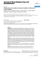
Figure 1.1 Scatterplot of age versus income overlaid with fitted regression curves.

is measured by 𝛽2 . Because age is expected to explain a considerable part of variability in income, we
expect 𝜎 2 to be significantly less than 𝜎u2 . A useful way of visualizing the model is with a scatterplot of
xi,2 and yi . Figure 1.1 shows such a graph based on a fictitious set of data for 200 individuals between the
ages of 16 and 60 and their monthly net income in euros. It is quite clear from the scatterplot that age
and income are positively correlated. If age is neglected, then the i.i.d. normal model for income results
in 𝜇̂ u = 1,797 euros and 𝜎̂ u = 1,320 euros. Using the techniques discussed below, the regression model
gives estimates 𝛽̂1 = −1,465, 𝛽̂2 = 85.4, and 𝜎̂ = 755, the latter being about 43% smaller than 𝜎̂ u . The
model implies that, conditional on the age x, the income Y is modeled as N(−1,465 + 85.4x, 7552 ). This
is valid only for 16 ⩽ x ⩽ 60; because of the negative intercept, small values of age would erroneously
imply a negative income. The fitted model y = 𝛽̂1 + 𝛽̂2 x is overlaid in the figure as a solid line.
Notice in Figure 1.1 that the linear approximation underestimates income for both low and high
age groups, i.e., income does not seem perfectly linear in age, but rather somewhat quadratic. To
accommodate this, we can add another regressor, xi,3 = x2i,2 , into the model, i.e., Yi = 𝛽1 + 𝛽2 xi,2 +
i.i.d.

𝛽3 xi,3 + 𝜖i , where 𝜖i ∼ N(0, 𝜎q2 ) and 𝜎q2 denotes the conditional variance based on the quadratic model.
It is important to realize that the model is still linear (in the constant, age, and age squared). The fitted
̂
model turns out to be Yi = 190 − 12.5xi,2 + 1.29xi,3 , with 𝜎̂ q = 733, which is about 3% smaller than 𝜎.
The fitted curve is shown in Figure 1.1 as a dashed line.
One caveat still remains with the model for income based on age: The variance of income appears
to increase with age. This is a typical finding with income data and agrees with economic theory. It
implies that both the mean and the variance of income are functions of age. In general, when the
variance of the regression error term is not constant, it is said to be heteroskedastic, as opposed
to homoskedastic. The generalized least squares extension of the linear regression model discussed
below can be used to address this issue when the structure of the heteroskedasticity as a function of

the X matrix is known.
In certain applications, the ordering of the dependent variable and the regressors is important
because they are observed in time, usually equally spaced. Because of this, the notation Yt will be
used, t = 1, … , T. Thus, (1.2) becomes
Yt = 𝛽1 xt,1 + 𝛽2 xt,2 + · · · + 𝛽k xt,k + 𝜖t ,

t = 1, 2, … , T,

where xt,i indicates the tth observation of the ith explanatory variable, i = 1, … , k, and 𝜖t is the tth
error term. In standard matrix notation, the model can be compactly expressed as
Y = X𝜷 + 𝝐,

(1.3)


The Linear Model

where [X]t,i = xt,i , i.e., with xt = (xt,1 , … , xt,k )′ ,
⎡ x1′
X=⎢ ⋮
⎢ ′
⎣ xT

⎤ ⎡
⎥ = ⎢⎢
⎥ ⎢
⎦ ⎣

x1,1
x2,1

⋮
xT,1

x1,2
x2,2
⋮
xT,2

···
···

x1,k
x2,k
⋮
xT,k

⎤
⎥
⎥,
⎥
⎦

𝝐 ∼ N(𝟎, 𝜎 2 I),

Y and 𝝐 are T × 1, X is T × k and 𝜷 is k × 1. The first column of X is usually 𝟏, the column of ones.
Observe that Y ∼ N(X𝜷, 𝜎 2 I).
An important special case of (1.3) is with k = 2 and xt,1 = 1. Then Yt = 𝛽1 + 𝛽2 Xt + 𝜖t , t = 1, … , T,
is referred to as the simple linear regression model. See Problems 1.1 and 1.2.

1.2 Ordinary and Generalized Least Squares

1.2.1

Ordinary Least Squares Estimation

The most popular way of estimating the k parameters in 𝜷 is the method of least squares,2 which
̂ = arg min S(𝜷), where
takes 𝜷
S(𝜷) = S(𝜷; Y , X) = (Y − X𝜷)′ (Y − X𝜷) =

T
∑

(Yt − xt′ 𝜷)2 ,

(1.4)

t=1

and we suppress the dependency of S on Y and X when they are clear from the context.
Assume that X is of full rank k. One procedure to obtain the solution, commonly shown in most
books on regression (see, e.g., Seber and Lee, 2003, p. 38), uses matrix calculus; it yields 𝜕 S(𝜷)∕𝜕𝜷 =
−2X′ (Y − X𝜷), and setting this to zero gives the solution
̂ = (X′ X)−1 X′ Y.
𝜷

(1.5)

This is referred to as the ordinary least squares, or o.l.s., estimator of 𝜷. (The adjective “ordinary” is
used to distinguish it from what is called generalized least squares, addressed in Section 1.2.3 below.)
̂ is also the solution to what are referred to as the normal equations, given by

Notice that 𝜷
̂ = X′ Y.
X′ X𝜷

(1.6)

To verify that (1.5) indeed corresponds to the minimum of S(𝜷), the second derivative is checked for
positive definiteness, yielding 𝜕 2 S(𝜷)∕𝜕𝜷𝜕𝜷 ′ = 2X′ X, which is necessarily positive definite when X is
̂ reduces
full rank. Observe that, if X consists only of a column of ones, which we write as X = 𝟏, then 𝜷
̂ reduces to X−1 Y, with S(𝜷)
̂ = 0.
to the mean, Ȳ , of the Yt . Also, if k = T (and X is full rank), then 𝜷
̂
Observe that the derivation of 𝜷 in (1.5) did not involve any explicit distributional assumptions.
One consequence of this is that the estimator may not have any meaning if the maximally existing
moment of the {𝜖t } is too low. For example, take X = 𝟏 and {𝜖t } to be i.i.d. Cauchy; then 𝛽̂ = Ȳ is
a useless estimator. If we assume that the first moment of the {𝜖t } exists and is zero, then, writing
̂ is unbiased:
̂ = (X′ X)−1 X′ (X𝜷 + 𝝐) = 𝜷 + (X′ X)−1 X′ 𝝐, we see that 𝜷
𝜷
̂ = 𝜷 + (X′ X)−1 X′ 𝔼[𝝐] = 𝜷.
𝔼[𝜷]

(1.7)

2 This terminology dates back to Adrien-Marie Legendre (1752–1833), though the method is most associated in its origins
with Carl Friedrich Gauss, (1777–1855). See Stigler (1981) for further details.

7

8

Linear Models and Time-Series Analysis

̂ ∣ 𝜎 2 ) is given by
Next, if we have existence of second moments, and 𝕍 (𝝐) = 𝜎 2 I, then 𝕍 (𝜷
̂ − 𝜷)(𝜷
̂ − 𝜷)′ ∣ 𝜎 2 ] = (X′ X)−1 X′ 𝔼[𝝐𝝐 ′ ]X(X′ X)−1 = 𝜎 2 (X′ X)−1 .
𝔼[(𝜷

(1.8)

̂ has the smallest variance among all linear unbiased estimators; this result is often
It turns out that 𝜷
̂ is the best linear unbireferred to as the Gauss–Markov Theorem, and expressed as saying that 𝜷
ased estimator, or BLUE. We outline the usual derivation, leaving the straightforward details to the
∗
̂ = A′ Y, where A′ is a k × T nonstochastic matrix (it can involve X, but not Y). Let
reader. Let 𝜷
∗
̂ ] and show that the unbiased property implies that D′ X = 𝟎.
D = A − X(X′ X)−1 . First calculate 𝔼[𝜷
∗
∗
̂ ∣ 𝜎 2 ) = 𝕍 (𝜷
̂ ∣ 𝜎 2 ) + 𝜎 2 D′ D. The result follows because
̂ ∣ 𝜎 2 ) and show that 𝕍 (𝜷
Next, calculate 𝕍 (𝜷

′
D D is obviously positive semi-definite and the variance is minimized when D = 𝟎.
In many situations, it is reasonable to assume normality for the {𝜖t }, in which case we may easily
estimate the k + 1 unknown parameters 𝜎 2 and 𝛽i , i = 1, … , k, by maximum likelihood. In particular, with
{
}
1
fY (y) = (2𝜋𝜎 2 )−T∕2 exp − 2 (y − X𝜷)′ (y − X𝜷) ,
(1.9)
2𝜎
and log-likelihood
T
1
T
log(2𝜋) − log(𝜎 2 ) − 2 S(𝜷),
2
2
2𝜎
where S(𝜷) is given in (1.4), setting
𝓁(𝜷, 𝜎 2 ; Y) = −

𝜕𝓁
2
= − 2 X′ (Y − X𝜷) and
𝜕𝜷
2𝜎

(1.10)

𝜕𝓁

T
1
= − 2 + 4 S(𝜷)
𝜕𝜎 2
2𝜎
2𝜎

̂
to zero yields the same estimator for 𝜷 as given in (1.5) and 𝜎̃ 2 = S(𝜷)∕T.
It will be shown in Section
2
1.3.2 that the maximum likelihood estimator (hereafter m.l.e.) of 𝜎 is biased, while estimator
̂
𝜎̂ 2 = S(𝜷)∕(T
− k)

(1.11)

is unbiased.
̂ is a linear function of Y, (𝜷
̂ ∣ 𝜎 2 ) is multivariate normally distributed, and thus characterized
As 𝜷
̂ ∣ 𝜎 2 ) ∼ N(𝜷, 𝜎 2 (X′ X)−1 ).
by its first two moments. From (1.7) and (1.8), it follows that (𝜷
1.2.2

Further Aspects of Regression and OLS

The coefficient of multiple determination, R2 , is a measure many statisticians love to hate. This
animosity exists primarily because the widespread use of R2 inevitably leads to at least occasional misuse.

(Richard Anderson-Sprecher, 1994)
̂ is referred to as the residual sum of squares, abbreviated RSS. The
In general, the quantity S(𝜷)
∑T
̂t − Ȳ )2 , where the fitted value
explained sum of squares, abbreviated ESS, is defined to be t=1 (Y
′
̂ and the total (corrected) sum of squares, or TSS, is ∑T (Yt − Ȳ )2 . (Annoyingly,
̂t ∶= x 𝜷,
of Yt is Y
t=1
t
both words “error” and “explained” start with an “e”, and some presentations define SSE to be the error
sum of squares, which is our RSS; see, e.g., Ravishanker and Dey, 2002, p. 101.)


The Linear Model

The term corrected in the TSS refers to the adjustment of the Yt for their mean. This is done because
the mean is a “trivial” regressor that is not considered to do any real explaining of the dependent
∑T
variable. Indeed, the total uncorrected sum of squares, t=1 Yt2 , could be made arbitrarily large just
by adding a large enough constant value to the Yt , and the model consisting of just the mean (i.e.,
an X matrix with just a column of ones) would have the appearance of explaining an arbitrarily large
amount of the variation in the data.
̂t ) + (Y
̂t − Ȳ ), it is not immediately obvious that
While certainly Yt − Ȳ = (Yt − Y
T
∑

(Yt − Ȳ )2 =

t=1

T
∑

̂t )2 +
(Yt − Y

t=1

T
∑

̂t − Ȳ )2 ,
(Y

t=1

i.e.,
TSS = RSS + ESS.

(1.12)

This fundamental identity is proven below in Section 1.3.2.
A popular statistic that measures the fraction of the variability of Y taken into account by a linear
regression model that includes a constant, compared to use of just a constant (i.e., Ȳ ), is the coefficient
of multiple determination, designated as R2 , and defined as

R2 =

̂ Y, X)
S(𝜷,
ESS
RSS
=1−
=1−
,
TSS
TSS
S(Ȳ , Y, 𝟏)

(1.13)

where 𝟏 is a T-length column of ones. The coefficient of multiple determination R2 provides a measure
of the extent to which the regressors “explain” the dependent variable over and above the contribution
from just the constant term. It is important that X contain a constant or a set of variables whose linear
combination yields a constant; see Becker and Kennedy (1992) and Anderson-Sprecher (1994) and the
references therein for more detail on this point.
By construction, the observed R2 is a number between zero and one. As with other quantities
associated with regression (such as the nearly always reported “t-statistics” for assessing individual
“significance” of the regressors), R2 is a statistic (a function of the data but not of the unknown parameters) and thus is a random variable. In Section 1.4.4 we derive the F test for parameter restrictions.
With J such linear restrictions, and ̂
𝜸 referring to the restricted estimator, we will show (1.88), repeated
here, as
F=

̂
[S(̂

𝜸 ) − S(𝜷)]∕J
∼ F(J, T − k),
̂
S(𝜷)∕(T
− k)

(1.14)

under the null hypothesis H0 that the J restrictions are true. Let J = k − 1 and ̂
𝜸 = Ȳ , so that the
restricted model is that all regressor coefficients, except the constant are zero. Then, comparing (1.13)
and (1.14),
F=

T − k R2
,
k − 1 1 − R2

or

R2 =

(k − 1)F
.
(T − k) + (k − 1)F

(1.15)

Dividing the numerator and denominator of the latter expression by T − k and recalling the relationship between F and beta random variables (see, e.g., Problem I.7.20), we immediately have that
(

)
k−1 T −k
R2 ∼ Beta
,
,
(1.16)
2
2

9


10

Linear Models and Time-Series Analysis

so that 𝔼[R2 ] = (k − 1)∕(T − 1) from, for example, (I.7.12). Its variance could similarly be stated. Recall
that its distribution was derived under the null hypothesis that the k − 1 regression coefficients are
zero. This implies that R2 is upward biased, and also shows that just adding superfluous regressors
will always increase the expected value of R2 . As such, choosing a set of regressors such that R2 is
maximized is not appropriate for model selection.
However, the so-called adjusted R2 can be used. It is defined as
T −1
.
(1.17)
T −k
Virtually all statistical software for regression will include this measure. Less well known is that it
has (like so many things) its origin with Ronald Fisher; see Fisher (1925). Notice how, like the Akaike
information criterion (hereafter AIC) and other penalty-based measures applied to the obtained log
likelihood, when k is increased, the increase in R2 is offset by a factor involving k in R2adj .

Measure (1.17) can be motivated in (at least) two ways. First, note that, under the null hypothesis,
(
)
k−1 T −1
𝔼[R2adj ] = 1 − 1 −
= 0,
T −1 T −k
R2adj = 1 − (1 − R2 )

providing a perfect offset to R2 ’s expected value simply increasing in k under the null. A second way
is to note that, while R2 = 1 − RSS∕TSS from (1.13),
R2adj = 1 −

RSS∕(T − k)
𝕍̂ (̂
𝝐)
,
=1−
TSS∕(T − 1)
𝕍̂ (Y)

the numerator and denominator being unbiased estimators of their respective variances, recalling
(1.11). The use of R2adj for model selection is very similar to use of other measures, such as the (corrected) AIC and the so-called Mallows’ Ck ; see, e.g., Seber and Lee (2003, Ch. 12) for a very good
discussion of these, and other criteria, and the relationships among them.
Section 1.2.3 extends the model to the case in which Y = X𝜷 + 𝝐 from (1.3), but 𝝐 ∼ N(𝟎, 𝜎 2 𝚺),
where 𝚺 is a known, positive definite variance–covariance matrix. There, an appropriate expression
for R2 will be derived that generalizes (1.13). For now, the reader is encouraged to express R2 in (1.13)
as a ratio of quadratic forms, assuming 𝝐 ∼ N(𝟎, 𝜎 2 𝚺), and compute and plot its density for a given X
and 𝚺, such as given in (1.31) for a given value of parameter a, as done in, e.g., Carrodus and Giles
(1992). When a = 0, the density should coincide with that given by (1.16).

We end this section with an important remark, and an important example.
Remark It is often assumed that the elements of X are known constants. This is quite plausible in
designed experiments, where X is chosen in such a way as to maximize the ability of the experiment
to answer the questions of interest. In this case, X is often referred to as the design matrix. This
will rarely hold in applications in the social sciences, where the xt′ reflect certain measurements and
are better described as being observations of random variables from the multivariate distribution
describing both xt′ and Yt . Fortunately, under certain assumptions, one may ignore this issue and
proceed as if xt′ were fixed constants and not realizations of a random variable.
Assume matrix X is no longer deterministic. Denote by X an outcome of random variable , with
kT-variate probability density function (hereafter p.d.f.) f (X ; 𝜽), where 𝜽 is a parameter vector. We
require the following assumption: