Polarization observables in WZ production at the 13 TEV Lhc: Inclusive case
Bạn đang xem bản rút gọn của tài liệu. Xem và tải ngay bản đầy đủ của tài liệu tại đây (451.86 KB, 13 trang )
Communications in Physics, Vol. 30, No. 1 (2020), pp. 35-47
DOI:10.15625/0868-3166/30/1/14461
POLARIZATION OBSERVABLES IN WZ PRODUCTION AT THE 13 TEV
LHC: INCLUSIVE CASE
JULIEN BAGLIO1 AND LE DUC NINH2,†
1 CERN,
Theoretical Physics Department, CH-1211 Geneva 23, Switzerland
For Interdisciplinary Research in Science and Education,
ICISE, 590000 Quy Nhon, Vietnam
2 Institute
† E-mail:
Received 4 November 2019
Accepted for publication 21 January 2020
Published 28 February 2020
Abstract. We present a study of the polarization observables of the W and Z bosons in the process
pp → W ± Z → e± νe µ + µ − at the 13 TeV Large Hadron Collider. The calculation is performed
at next-to-leading order, including the full QCD corrections as well as the electroweak corrections, the latter being calculated in the double-pole approximation. The results are presented in
the helicity coordinate system adopted by ATLAS and for different inclusive cuts on the di-muon
invariant mass. We define left-right charge asymmetries related to the polarization fractions between the W + Z and W − Z channels and we find that these asymmetries are large and sensitive
to higher-order effects. Similar findings are also presented for charge asymmetries related to a
P-even angular coefficient.
Keywords: diboson production, LHC, next-to-leading-order corrections, polarization, standard
model.
Classification numbers: 12.15.-y; 14.70.Fm 14.70.Hp.
I. INTRODUCTION
In the framework of the Standard Model (SM) of particle physics the W boson only interacts
with left-handed fermions while the Z boson interacts with both left- and right-handed fermions,
albeit with different coupling strengths. This allows for a polarized production at hadron colliders
and in particular at the CERN Large Hadron Collider (LHC), leading to asymmetries in the angular
distributions of the leptonic decay products of the electroweak gauge bosons. Measuring these
c 2020 Vietnam Academy of Science and Technology
36
POLARIZATION OBSERVABLES IN WZ PRODUCTION AT THE 13 TEV LHC: INCLUSIVE CASE
asymmetries is a probe of the underlying polarization of the gauge bosons and eventually of their
spin structure.
The pair production of W and Z bosons has been the subject of recent experimental studies [1] in order to gain information about the polarization of the gauge bosons. On the theory
side, leading order (LO) studies began a while ago [2, 3] before being revived [4] and studied
in a recent paper [5] in the process pp → W ± Z → e± νe µ + µ − at next-to-leading order (NLO)
including both QCD and electroweak (EW) corrections, the latter being calculated in the doublepole approximation (DPA). This approximation works remarkably well in this process as shown
by the comparison performed in Ref. [5] with the exact NLO EW calculation for the differential
distributions [6], which completed the NLO EW picture after the on-shell predictions presented in
Refs. [7, 8]. Note that for the production process itself the QCD corrections are known up to nextto-next-to-leading order in QCD [9–12]. In Ref. [5] the extensive study of the NLO QCD+EW
predictions for gauge boson polarization observables, namely polarization fractions and angular
coefficients, was done in two different coordinate systems, the Collins-Soper [13] and helicity [14]
coordinate systems. However, in the recent experimental analysis by ATLAS with 13 TeV LHC
data [1], a different coordinate system was used, namely a modified helicity coordinate system in
which the z axis is now defined as the direction of the W (or Z) boson as seen in the W Z center-ofmass system. In addition, the study in Ref. [5] introduced fiducial polarization observables, which
have the advantage of being much simpler to define and calculate (and should also be measurable),
but are not the observables that are measured by the experiments yet.
The goal of this paper is to make one step closer to the experimental setup by using the
modified helicity coordinate system and giving predictions in an inclusive setup, using as default
the experimental total phase space defined by ATLAS at the 13 TeV LHC. It is noted that polarization fractions at the total-phase-space level are needed in [1] to simulate the helicity templates
necessary to extract the polarization fractions in the fiducial-phase-space region.
In addition to providing results for polarization fractions and angular coefficients, we also
V and C V with V = W, Z) that are large at the NLO
present two charge asymmetries (denoted ALR
3
QCD+EW accuracy, which are sensitive to either the QCD or the EW corrections depending on the
asymmetry and on the gauge boson that is under consideration. These asymmetries help to probe
the underlying spin structure of the gauge bosons and should be measurable in the experiments.
We use the same calculation setup presented in Ref. [5], and our calculation is exact at NLO QCD
using the program VBFNLO [15, 16] while the EW corrections are calculated in the DPA presented
in Ref. [5].
Compared to our previous work [5], the differences in this paper are the phase-space cuts
and the definition of the coordinate system to determine the lepton angles. Instead of using more
realistic fiducial cuts as in Ref. [5], we use here only one simple cut on the muon-pair invariant
mass, e.g. 66 GeV < mµ + µ − < 116 GeV. The benefit of considering this inclusive phase space is
that the “genuine” polarization observables can be easily calculated using the projection method
defined in Ref. [5]. The word “genuine” here means that the observables are not affected by cuts
on the kinematics of the individual leptons such as pT, or η . This inclusive case may therefore
provide more insights into various effects, which are difficult to understand when complicated
kinematical cuts on the individual leptons are present.
We discuss in Sec. II the polarization observables of a massive gauge boson in the total
phase space and our method to calculate them. The coordinate system that we use to determine
JULIEN BAGLIO AND LE DUC NINH
37
the lepton angles is also defined. In Sec. III numerical results for the polarization fractions and
angular coefficients are presented for both W + Z and W − Z channels. From this, results for various
charge asymmetries between the two channels are calculated. We finally conclude in Sec. IV.
II. POLARIZATION OBSERVABLES
The definition of polarization observables and calculational details have been all given in
Ref. [5] and we will not repeat them extensively. For an easy reading of this paper, we provide
here a brief summary of polarization observables and the main calculational details. This will be
needed to understand the numerical results presented in the next section. Polarization observables
associated with a massive gauge boson are constructed based on the angular distribution of its
decay product, typically a charged lepton (electron or muon). In the rest frame of the gauge
boson, this distribution reads [13, 17, 18]
3
1
dσ
=
(1 + cos2 θ ) + A0 (1 − 3 cos2 θ ) + A1 sin(2θ ) cos φ
σ dcos θ dφ
16π
2
1 2
+ A2 sin θ cos(2φ ) + A3 sin θ cos φ + A4 cos θ
2
+ A5 sin2 θ sin(2φ ) + A6 sin(2θ ) sin φ + A7 sin θ sin φ ,
(1)
where θ and φ are the lepton polar and azimuthal angles, respectively, in a particular coordinate
system that needs to be specified. A0−7 are dimensionless angular coefficients independent of θ
and φ . A0−4 are called P-even and A5−7 P-odd according to the parity transformation where φ
flips sign while θ remains unchanged [19, 20]. We also note here that A5−7 are proportional to the
imaginary parts of the spin-density matrix of the W and Z bosons in the DPA at LO [5, 21, 22].
This is important to understand why the values of these coefficients are very small, as will be later
shown.
We can also define the polarization fractions f W /Z by integrating over φ ,
±
±
±
3
dσ
= (1 ∓ cos θe± )2 fLW + (1 ± cos θe± )2 fRW + 2 sin2 θe± f0W ,
σ dcos θe±
8
3
dσ
= (1 + cos2 θµ − + 2c cos θµ − ) fLZ + (1 + cos2 θµ − − 2c cos θµ − ) fRZ + 2 sin2 θµ − f0Z .
σ dcos θµ −
8
(2)
The upper signs are for W + and the lower signs are for W − . The parameter c reads
c=
2
g2L − g2R
1 − 4sW
=
,
2 + 8s4
g2L + g2R 1 − 4sW
W
2
sW
= 1−
2
MW
,
MZ2
(3)
occurring because the Z boson decays into both left- and right-handed leptons. Relations between
V
the polarization fractions fL,R,0
with V = W, Z and the angular coefficients are therefore obvious,
where bW ±
1
1
1
fLV = (2 − AV0 + bV AV4 ), fRV = (2 − AV0 − bV AV4 ), f0V = AV0 ,
4
4
2
= ∓1, bZ = 1/c. From this, we get
bV
fLV + fRV + f0V = 1, fLV − fRV = AV4 .
2
(4)
(5)
38
POLARIZATION OBSERVABLES IN WZ PRODUCTION AT THE 13 TEV LHC: INCLUSIVE CASE
These coefficients are named polarization observables because they are directly related to
the spin-density matrix of the W and Z bosons in the DPA and at LO as above mentioned. In
order to calculate them, we first have to calculate the distributions dσ /(d cos θ dφ ), or simply the
distributions dσ /(d cos θ ) if only the polarization fractions are of interest. This can be computed
order by order in perturbation theory. We have calculated this up to the NLO QCD + EW accuracy
using the same calculation setup as in Ref. [5]. The NLO QCD results are exact, using the full
amplitudes as provided by the VBFNLO program. The NLO EW corrections are however calculated
in the DPA as presented in Ref. [5]. In the DPA, only the double-resonant Feynman diagrams
are taken into account. Single-resonant diagrams including γ ∗ → µ + µ − (as shown in Fig. 1a) or
W → 2 2ν (as shown in Fig. 1b) are neglected. Moreover, even for the double-resonant diagrams,
off-shell effects are not included. In the next section we will also provide results at LO using the
DPA (dubbed DPA LO) or using the full amplitudes (dubbed simply LO).
a) q¯
e−
W−
W
q′
b) q¯
q′
Z/γ
−
ν¯e
µ−
q¯
q′
q′
W−
e−
Z/γ
ν¯e
µ−
µ+
W−
ν¯e
Z
e−
ν¯e
µ−
µ+
µ+
q¯
q′
ν¯e
W−
e−
Z/γ
e−
µ−
µ+
q¯
q′
µ−
W−
ν¯µ
W−
µ+
ν¯e
e−
Fig. 1. Double and single resonant diagrams at leading order. Group a) includes both
double and single resonant diagrams, while group b) is only single resonant.
Finally, we specify the coordinate system to determine the angle θ and φ . Differently from
Ref. [5], we use here the modified helicity coordinate system. The only difference compared to
the helicity system is the direction of the z axis: instead of being the gauge boson flight direction
in the laboratory frame as chosen in Refs. [5, 14], it is now the gauge boson flight direction in
the W Z center-of-mass frame. This modified helicity coordinate system is also used in the latest
ATLAS paper presenting results for the polarization observables in the W Z channel [1]. We think
the modified helicity system is a better choice when studying the spin correlations of the two
gauge bosons. However, for polarizations of a single gauge boson, the helicity system is more
advantageous because of a better reconstruction of the Z boson direction in the laboratory frame.
In both cases, an algorithm to determine the momentum of the W boson from its decay products is
still needed, which has been done in [1]. We note that the spin correlations of the two gauge bosons
are fully included in our calculation. However, we do not provide separately numerical results for
these effects in this paper because the need for them is not urgent as the current experimentalstatistic level is still limited to be sensitive to those effects. Nevertheless, we choose to use the
modified helicity system to be closer to the ATLAS measurement and to prepare for the future
studies of those spin correlations.
JULIEN BAGLIO AND LE DUC NINH
39
III. NUMERICAL RESULTS
The input parameters are
Gµ = 1.16637 × 10⁻⁵ GeV−2 , MW = 80.385 GeV, MZ = 91.1876 GeV,
ΓW = 2.085 GeV, ΓZ = 2.4952 GeV, Mt = 173 GeV, MH = 125 GeV,
(6)
which are the same as the ones used in Ref. [5]. The masses of the leptons and the light quarks,
i.e. all but the top mass, are approximated as zero. This is justified because our results
√ are 2insen(1 −
sitive to those small masses. The electromagnetic coupling is calculated as αGµ = 2Gµ MW
2
2
MW /MZ )/π. For the factorization and renormalization scales, we use µF = µR = (MW + MZ )/2.
Moreover, the parton distribution functions (PDF) are calculated using the Hessian set
LUXqed17_plus_PDF4LHC15_nnlo_30 [23–32] via the library LHAPDF6 [33].
√
We will give results for the LHC running at a center-of-mass energy s = 13 TeV, for both
e+ νe µ + µ − and e− ν¯ e µ + µ − final states, also denoted, respectively, as W + Z and W − Z channels
for conciseness. We treat the extra parton occurring in the NLO QCD corrections inclusively and
we do not apply any jet cuts. We also consider the possibility of lepton-photon recombination,
where we redefine the momentum of a given charged lepton as being p = p + pγ if ∆R( , γ) ≡
(∆η)2 + (∆φ )2 < 0.1. We use for either e or µ. If not otherwise stated, the default phase-space
cut is
66 GeV < mµ + µ − < 116 GeV,
(7)
which is used in Ref. [1, 34] to define the experimental total phase space. With this cut, we obtain
the following result for the total cross section
σWtot.± Z,NLO QCD+EW = 45.8 ± 0.7 (PDF) + 2.2/ − 1.8 (scale) pb,
(8)
where we have used Br(W → eνe ) = 10.86% and Br(Z → µ + µ − ) = 3.3658% as provided in
Ref. [35] to unfold the cross section as done in Ref. [1]. This result is to be compared with
σWtot.± Z,ATLAS = 51.0 ± 2.4 pb as reported in Ref. [1], showing a good agreement at the 1.6σ level.
The agreement becomes even much better when the next-to-next-to-leading order QCD corrections, of the order of a +11% on top of the NLO QCD results at 13 TeV for our scale choice, are
taken into account [11]. We note that the EW corrections to the total cross section are completely
negligible (at the sub-permil level) because of the cancellation between the negative corrections to
the qq
¯ channels and the positive corrections to the qγ channels, in agreement with the finding in
Ref. [8].
III.1. Angular distributions and polarization fractions
We first present here results for the cos θ distributions, from which the polarization fractions
are calculated. They are shown in Fig. 2, where the LO, NLO QCD, and NLO QCD+EW distributions are separately provided. The bands indicate the total theoretical uncertainty calculated as
a linear sum of PDF and scale uncertainties at NLO QCD. The K factor defined as
KNLOQCD =
dσNLOQCD
dσLO
(9)
40
POLARIZATION OBSERVABLES IN WZ PRODUCTION AT THE 13 TEV LHC: INCLUSIVE CASE
80
pp→e + νe µ + µ − | s = 13TeV | ATLAStot
NLOQCD
NLOQCDEW
LO
70
[fb]
[fb]
60
50
40
KNLOQCD
1.5
2
0
2
4
δq¯q
0.5
45
0.0
δqγ
0.0
cos(θµWZ )
δq¯DPA
q
δqγDPA
0.5
30
20
20
2.0
1.8
1.6
1.4
2
0
2
4
1.9
1.7
1.5
2
0
2
4
0.0
cos(θeWZ )
δqγDPA
δEW [%]
KNLOQCD
25
δq¯DPA
q
NLOQCD
NLOQCDEW
LO
35
25
δqγ
pp→e − ν¯e µ + µ − | s = 13TeV | ATLAStot
40
[fb]
[fb]
45
30
0.5
δq¯q
−
NLOQCD
NLOQCDEW
LO
δq¯q
NLOQCD
NLOQCDEW
LO
0.5
pp→e − ν¯e µ + µ − | s = 13TeV | ATLAStot
35
KNLOQCD
δqγDPA
pp→e + νe µ + µ − | s = 13TeV | ATLAStot
1.9
1.7
1.5
2
0
2
4
0.5
cos(θeWZ )
40
δEW [%]
δq¯DPA
q
δqγ
δEW [%]
1.7
δEW [%]
KNLOQCD
30
70
65
60
55
50
45
40
35
30
δq¯q
0.5
0.5
δqγ
0.0
cos(θµWZ )
δq¯DPA
q
δqγDPA
0.5
−
Fig. 2. Distributions of the cos θ distributions of the (anti)electron (left column) and
the muon (left column) for the process W + Z (top row) and W − Z (bottom row). The
upper panels show the absolute values of the cross sections at LO (in green), NLO QCD
(red), and NLO QCD+EW (blue). The middle panels display the ratio of the NLO QCD
cross sections to the corresponding LO ones. The bands indicate the total theoretical
uncertainty calculated as a linear sum of PDF and scale uncertainties at NLO QCD. The
bottom panels show the NLO EW corrections (see text) calculated using DPA relative to
the LO (marked with plus signs) and DPA LO cross sections.
is shown in the middle panels together with the corresponding uncertainty bands. To quantify the
EW corrections, we define, as in Ref. [5], the following EW corrections
δqq
¯ =
NLOEW
d∆σqq
¯
dσ LO
,
δqγ =
NLOEW
d∆σqγ
,
dσ LO
(10)
JULIEN BAGLIO AND LE DUC NINH
41
where the EW corrections to the quark anti-quark annihilation processes and to the photon quark
induced processes are separated. The reason to show these corrections separately is to see to what
extent they cancel each other. For the case of on-shell W Z production, it has been shown in Ref. [8]
that this cancellation is large. In this work, since leptonic decays are included, the QED final state
photon radiation shifts the position of the di-muon invariant mass, leading to a shift in the photonradiated contribution to the δqq
¯ correction. This shift is negative, making the δqq
¯ correction more
negative. As a result, we see that the total EW correction δEW = δqq
+
δ
is
negative, while it
qγ
¯
is more positive in Ref. [8]. Another important difference between this work and Ref. [8] is that
different photon PDFs are used. This also changes the qγ contribution significantly.
In order to see the effects of the DPA approximation at LO, we replace the denominators in
Eq. (10) by the DPA LO results. This gives
DPA
=
δqq
¯
NLOEW
d∆σqq
¯
LO
dσDPA
,
DPA =
δqγ
NLOEW
d∆σqγ
,
LO
dσDPA
(11)
which are also shown in the bottom panels in Fig. 2 for the sake of comparison. The EW corrections δEW are the same when compared to DPA LO or LO, while in Ref. [5] there are some
differences especially at large negative cos θ values. The effect of inclusive cuts is thus here visible.
We see that the NLO QCD corrections are large, varying in the range from 40% to 100%
compared to the LO cross section, while the NLO EW corrections are very small in magnitude, as
already known [8]. However it is important to note that the shape of the angular distributions is
different between the EW corrections and the QCD corrections, a new feature which has an impact
on the polarization fractions. We see clearly that the QCD corrections are not constant, but the
shape distortion effect is not that large except in the cos θe− in the W − Z channel where the QCD
K–factor starts at KNLOQCD 1.5 for large negative cos θ values and reaches KNLOQCD 1.85 at
large positive values. The EW corrections also introduce some visible shape distortion effects.
Comparisons between the W + Z and W − Z channels are valuable as charge asymmetry observables
can be measured. In this context, it is interesting to notice that the QCD corrections are very
similar in the cos θµ − distributions, but very different in the cos θe distributions. Remarkably, the
opposite behaviors are observed in the EW corrections, for both qq
¯ and qγ corrections. The large
charge asymmetry in the QCD corrections to the cos θe distribution is most probably due to the qg
induced processes which first occur at NLO. On the other hand, the large effect observed in the
EW corrections to the cos θµ − distribution is due to the QED final state radiation. This means that
the charge asymmetries in W polarization fractions are more sensitive to the gluon PDF than in
the Z case.
From the above cos θ distributions, the polarization fractions are calculated. This result is
presented in Table 1, where PDF and scale uncertainties associated with the LO and NLO QCD
predictions are also calculated. To quantify the aforementioned higher-order effects on charge
asymmetry observables, we define here two observables,
V
ALR
=
qVW + Z − qVW − Z
,
qVW + Z + qVW − Z
B0V =
pVW + Z − pVW − Z
,
pVW + Z + pVW − Z
(12)
where qV = | fLV − fRV | and pV = | f0V |. Note that, absolute values are needed because, in general,
the fractions can get negative as shown in Ref. [5] for the case of the fiducial distributions in the
42
POLARIZATION OBSERVABLES IN WZ PRODUCTION AT THE 13 TEV LHC: INCLUSIVE CASE
Table 1. W and Z polarization fractions in the processes pp → e+ νe µ + µ − (upper rows)
and pp → e− νe µ + µ − (lower rows) at DPA LO, LO, NLO EW, NLO QCD, and NLO
QCD+EW. The PDF uncertainties (in parenthesis) and the scale uncertainties are provided
for the LO and NLO QCD results, all given on the last digit of the central prediction.
Method
fLW
f0W
fRW
fLZ
f0Z
fRZ
DPALO (W + Z)
0.515
0.153
0.332
0.333
0.144
0.522
LO (W + Z)
0.482(1)+1
−1
0.181(1)+1
−2
0.337(0.2)+1
−0.5
0.306(1)+1
−1
0.164(0.4)+1
−1
0.529(0.3)+0.3
−0.2
NLOEW (W + Z)
0.486
0.180
0.334
0.335
0.169
0.496
NLOQCD (W + Z)
0.471(1)+1
−1
0.218(1)+3
−3
0.311(1)+2
−2
0.338(1)+3
−3
0.209(1)+4
−3
0.453(1)+6
−6
NLOQCDEW (W + Z)
0.473
0.218
0.309
0.355
0.212
0.433
DPALO (W − Z)
0.329
0.158
0.513
0.520
0.150
0.331
LO (W − Z)
0.316(0.4)+1
−1
0.181(0.4)+1
−1
0.503(0.3)+1
−1
0.501(1)+1
−0.4
0.168(0.4)+1
−1
0.332(0.4)+1
−1
NLOEW (W − Z)
0.313
0.181
0.506
0.470
0.172
0.358
NLOQCD (W − Z)
0.344(1)+3
−2
0.225(1)+3
−3
0.431(1)+6
−6
0.478(1)+1
−2
0.208(1)+3
−3
0.314(1)+2
−2
NLOQCDEW (W − Z)
0.342
0.226
0.432
0.459
0.211
0.329
Table 2. Left-right charge asymmetries.
Asymmetry
W
ALR
Z
ALR
DPALO
LO
−27.0% −12.7%
0%
+13.8%
NLOEW NLOQCD NLOQCDEW
−11.9%
+17.9%
+29.6%
+29.1%
−17.6%
−25.0%
Collins-Soper coordinate system. Furthermore, since the three fractions sum to unity, only two
parameters are independent. From Table 1 we see that B0V is not interesting as this asymmetry
is very small, namely B0W ≈ −2% and B0Z ≈ +0.2% at NLO QCD+EW accuracy. However,
V are much larger, being A W ≈ +29% and A Z ≈ −25% at
the left-right charge asymmetries ALR
LR
LR
NLO QCD+EW accuracy. Results at DPA LO, LO, NLO EW and NLO QCD levels are provided
in Table 2, showing that these observables are very sensitive to off-shell and higher-order effects
as the left-right asymmetries are negligible in the DPA limit, being numerically at the per mill
level for the W case and even smaller for the Z case. Consistently with the above observations on
the distributions, we see that the W asymmetry is more sensitive to the QCD corrections, while the
Z asymmetry is more sensitive to the EW corrections. Note that the theory uncertainties cancel in
the ratios defining the left-right asymmetries and are then expected to be negligible. We will not
discuss them further.
We close this section by presenting in Table 3 the NLO QCD+EW results of the fractions
for different invariant mass windows of the muon pair. These cuts are named CUT-i, i = 1, . . . , 6,
corresponding respectively to (86 GeV, 96 GeV), (81 GeV, 101 GeV), (76 GeV, 106 GeV), (71
GeV, 111 GeV), (66 GeV, 116 GeV), and (60 GeV, 120 GeV). Note that CUT-5 is the default cut
JULIEN BAGLIO AND LE DUC NINH
43
Table 3. NLO QCD+EW W and Z polarization fractions at different cuts (see text).
Cut
fLW
f0W
fRW
fLZ
f0Z
fRZ
CUT-1 (W + Z) 0.475 0.218 0.307
0.360 0.217 0.424
CUT-2 (W + Z)
0.475 0.217 0.308
0.359 0.214 0.427
CUT-3 (W + Z) 0.475 0.217 0.308
0.357 0.213 0.429
CUT-4 (W + Z)
0.474 0.217 0.309
0.356 0.213 0.431
CUT-5 (W + Z)
0.473 0.218 0.309
0.355 0.212 0.433
CUT-6 (W + Z)
0.473 0.218 0.310
0.353 0.212 0.435
CUT-1 (W − Z) 0.341 0.227 0.432
0.455 0.215 0.329
CUT-2 (W − Z)
0.341 0.226 0.433
0.457 0.213 0.330
CUT-3 (W − Z) 0.341 0.226 0.433
0.458 0.212 0.330
CUT-4 (W − Z)
0.342 0.226 0.433
0.459 0.212 0.329
CUT-5 (W − Z)
0.342 0.226 0.432
0.459 0.211 0.329
CUT-6 (W − Z)
0.343 0.226 0.432
0.460 0.211 0.329
defined in Eq. (7), while CUT-6 is used by CMS [36] to define their total phase space. As expected,
we see that the W fractions are almost unchanged while the Z fractions vary more visibly. For the
Z fractions, the different behaviors between the W + Z and W − Z channels are interesting. While
the fRZ in the former case varies most strongly, it is almost unchanged in the latter. This unexpected
constant behavior is due to the opposite behaviors in the other fractions.
III.2. Angular coefficients
We now turn to the angular coefficients. Results for the (anti)electron are presented in
Table 4 and for the muon in Table 5 at LO, NLO QCD, NLO EW, and NLO QCD+EW levels.
The first thing to notice is that the values of the P-odd coefficients A5−7 are very small, but
non-vanishing. In order to see that they are indeed statistically non-zero, we show the DPA LO and
LO results together with statistical errors in Table 6 for the (anti)electron case. For completeness,
similar results for the muon case are also provided in Table 7. We see that those coefficients are
zero within the statistical error in the DPA. However, at LO, when full off-shell effects are taken
+
µ−
into account, they are all non-zero, except Ae5 and A5,W + Z where the results are very small. It
has been shown in [5, 21] that, in the DPA, A5−7 are proportional to the imaginary part of the
spin-density matrices. This means that in the zero-width limit (i.e. ΓV → 0) they are vanishing,
explaining why they are so small in the DPA. Note that, a finite width induces an off-shell effect,
but the full off-shell effects at LO include additionally new Feynman diagrams such as virtual
photon and single-resonant contributions. This explains why the values of the P-odd coefficients
are significantly larger at LO than at DPA LO. Results in Table 4 and Table 5 show that they
remain very small at NLO QCD+EW accuracy. Measuring them in experiments is therefore very
challenging (see [20] for a study on W -jet production at the LHC).
44
POLARIZATION OBSERVABLES IN WZ PRODUCTION AT THE 13 TEV LHC: INCLUSIVE CASE
Table 4. Angular coefficients of the e+ (upper rows) and e− (lower rows) distributions for
the final states e+ νe µ + µ − and e− ν¯ e µ + µ − , respectively, at LO, NLO EW, NLO QCD,
and NLO QCD+EW. The PDF uncertainties (in parenthesis) and the scale uncertainties
are provided for the LO and NLO QCD results, all given on the last digit of the central
prediction.
Method
LO (W + Z)
NLOEW (W + Z)
NLOQCD (W + Z)
NLOQCDEW (W + Z)
LO (W − Z)
NLOEW (W − Z)
NLOQCD (W − Z)
NLOQCDEW (W − Z)
A0
A1
A2
A3
A4
A5
A6
A7
+1
+4
+1
+1
+1
+0.1
+0.2
0.363(1)+3
−3 −0.049(1)−2 −0.232(1)−4 −0.102(2)−2 −0.289(1)−1 −0.0002(1)−1 −0.003(0.3)−0.01 −0.011(0.5)−0.03
−0.052
0.359
−0.215
−0.091
−0.304
−0.001
+6
+3
+7
+3
+2
0.436(1)+6
−5 −0.120(1)−6 −0.233(1)−2 −0.021(2)−7 −0.319(2)−3 0.0003(5)−0.4
−0.122
0.435
−0.222
−0.014
−0.328
−0.005
−0.007
−0.001(1)+0.01
−0.2
−0.001(0.4)+1
−1
−0.002
0.001
−0.0002
+2
+4
+4
+0.2
+0
+0
0.362(1)+3
−3 −0.067(1)−2 −0.253(1)−3 0.118(2)−3 −0.374(1)−0.2 0.002(0.2)−0.03 0.002(0.4)−0.1
−0.072
0.362
−0.232
0.127
−0.388
+5
+4
+7
+17
0.451(1)+7
−7 −0.131(1)−5 −0.233(2)−4 0.032(2)−8 −0.174(4)−16
−0.135
0.451
−0.219
0.037
−0.180
0.007(0.4)+0.2
−0.02
0.003
0.004
0.0005
0.001(1)+0.3
−0.1
0.001(0.4)+0.2
−0.1
−0.005(0.3)+1
−1
0.002
0.002
−0.009
Table 5. Same as Table 4 but for the µ − coefficients.
Method
LO (W + Z)
NLOEW (W + Z)
NLOQCD (W + Z)
NLOQCDEW (W + Z)
LO (W − Z)
NLOEW (W − Z)
NLOQCD (W − Z)
NLOQCDEW (W − Z)
A0
A1
A2
A3
+2
+3
0.329(1)+2
−3 −0.034(1)−2 −0.145(1)−2
−0.038
0.338
−0.136
+5
+2
0.418(1)+7
−7 −0.096(1)−6 −0.144(1)−2
−0.100
0.424
−0.139
0.032(1)+1
−1
A4
A5
0.008
−0.146
0.041
−0.069
0.010(1)+2
−2
−0.049(1)+4
−4
0.015
−0.033
0.014
+7
+2
+1
0.417(1)+6
−6 −0.071(1)−7 −0.164(1)−1 0.001(0.5)−1
−0.075
0.423
−0.160
0.002
A7
+87
+0.1
+0.05
−0.096(0.3)+0.4
−0.3 0.000004(209)−83 −0.011(0.2)−0.1 0.013(0.2)−0.2
−0.0005
−0.012
0.013
+0.2
+0.2
0.0002(10)+2
−0.04 −0.008(0.3)−0.2 0.009(0.2)−0.3
−0.0002
+2
+2
+0.2
+0.2
0.335(1)+3
−3 0.013(1)−2 −0.153(1)−2 0.012(0.4)−0.1 0.072(0.3)−0.2
0.344
A6
0.004(0.2)+0.1
−0.04
−0.009
0.009
+0.1
0.009(0.2)+0.1
−0.1 0.014(0.2)−0.2
0.048
0.004
0.011
0.014
0.070(0.5)+0.3
−0.3
0.002(0.5)+0.2
−0.1
0.006(1)+0.2
−0.2
0.009(1)+0.3
−0.3
0.056
0.003
0.007
0.009
We now focus on the P-even coefficients A1−4 . Results at the NLO QCD+EW accuracy in
Table 4 and Table 5 show that they are large, hence should be measureable. EW corrections are
µ−
µ−
significant for A3 and A4 due to the radiative corrections to the Z → µ + µ − decay, as found in
Ref. [5] using more exclusive cuts.
Similarly to the previous section, we can define various charge asymmetries as
CiV
=
rVi,W + Z − rVi,W − Z
rVi,W + Z + rVi,W − Z
µ−
e
Z
, rW
i = |Ai |, ri = |Ai |, i = 1, . . . , 7.
(13)
JULIEN BAGLIO AND LE DUC NINH
45
Table 6. Angular coefficients of the e+ (upper rows) and e− (lower rows) distributions
for the final states e+ νe µ + µ − and e− ν¯ e µ + µ − , respectively, at DPA LO and LO. The
numbers in square brackets represent the statistical error, when it is significant.
Method
A0
A1
A2
A3
−0.030
−0.286
0.092
−0.049
−0.232 −0.102 −0.289
−0.0002[5]
−0.0034[4]
−0.011
DPALO (W − Z) 0.317 −0.0023[2] −0.295 −0.082 −0.367
0.00001[38]
−0.0001[2]
0.0001[2]
0.0024[4]
0.0024[3]
0.0067[2]
A6
A7
DPALO (W + Z) 0.306
LO (W + Z)
LO (W − Z)
0.363
0.362
−0.066
−0.254
0.118
A4
A5
A6
A7
−0.368 −0.00001[40] −0.0001[2] 0.00005[19]
−0.374
Table 7. Same as Table 6 but for the µ − distributions.
Method
A0
DPALO (W + Z) 0.289
LO (W + Z)
A2
A3
A4
A5
0.037
−0.183
−0.026
−0.081
−0.0001[2]
0.032
−0.096
0.0001[4]
0.329 −0.034 −0.145
DPALO (W − Z) 0.299
LO (W − Z)
A1
0.336
0.026
−0.188 −0.0085[1]
0.081
0.013
−0.154
0.072
0.012
−0.0001[1] 0.00001[17]
−0.011
0.013
−0.00003[19] −0.0001[2] 0.00002[14]
0.0041[8]
0.0091[4]
0.014
Because of the relations between fL,R,0 and A0,4 presented in Eq.(4), the asymmetries C0V and C4V
V , respectively. Looking at Table 4 and Table 5 we see that C V and C V
are identical to B0V and ALR
3
4
V in this discussion because they are very difficult
are the most interesting. Note that we ignore C5−7
to measure. Similar to Table 2, values for C3V in different approximations are provided in Table 8.
V , this asymmetry is much larger. Another interesting difference is the value at
Compared to ALR
V , it is large for C V , reaching +51% for the Z case,
DPA LO. While it is almost vanishing for ALR
3
suggesting very different origins. This is indeed the case because A3 is related to the off-diagonal
entries of the spin-density matrices at DPA LO, while A4 comes from the diagonal ones [5]. This
is also why the value of A3 is much smaller than that of A4 . All in all, we see that the value of C3V
is much larger hence could be an additional probe of the spin structure of the gauge bosons, but
V because of difficulties in measuring A .
this observable is more difficult to measure than ALR
3
Table 8. Charge asymmetries in the coefficient A3 .
Asymmetry DPALO
C3W
+0.057
C3Z
+0.507
LO
−0.073
+0.455
NLOEW NLOQCD NLOQCDEW
−0.165
+0.491
−0.208
+0.818
−0.451
+0.765
46
POLARIZATION OBSERVABLES IN WZ PRODUCTION AT THE 13 TEV LHC: INCLUSIVE CASE
IV. CONCLUSIONS
In this paper, we have presented results for polarization fractions and angular coefficients
up to the NLO QCD+EW accuracy in the process pp → e± νe µ + µ − at the 13 TeV LHC. We have
used by default the total phase space adopted by ATLAS in their latest 13 TeV analysis of the W
and Z polarization observables, measured in the modified helicity coordinate system where the
z-axis is defined as the gauge boson flight direction in the W Z center-of-mass frame. Our LO and
NLO QCD results include full off-shell effects while the EW corrections have been calculated in
the double-pole approximation.
W /Z
We have defined left-right charge asymmetries ALR out of the polarization fractions that
W is sensitive to the QCD corrections
are very sensitive to higher-order effects, in particular ALR
Z
while ALR is sensitive to the EW corrections. This sensitivity can be related to the shape of the
higher-order corrections to the angular distributions underlying the calculations of the polarization
fractions. These asymmetries are found to be large at NLO QCD+EW order, of the order of +29%
for the W boson and −25% for the Z boson, that should be measurable at the LHC.
We have also defined similar charge asymmetries for the angular coefficients themselves
and we have found that the asymmetries related to the P-even coefficient A3 can also be very large,
of the order of −45% for the W boson and +78% for the Z boson, and could be additional probes
of the polarization structure of the underlying dynamics, even if they are more difficult to measure
than the left-right charge asymmetries. The EW corrections are also found to be sizable in these
A3 charge asymmetries.
This work is a step towards a study of the polarization observables that is as close as possible
to the current experimental setup in ATLAS.
ACKNOWLEDGMENT
This work is funded by the Vietnam National Foundation for Science and Technology Development (NAFOSTED) under grant number 103.01-2017.78. We are grateful to Emmanuel
Sauvan for fruitful discussions.
REFERENCES
[1]
[2]
[3]
[4]
[5]
[6]
[7]
[8]
[9]
[10]
[11]
[12]
[13]
[14]
[15]
M. Aaboud et al., Eur. Phys. J. C79 (2019) 535.
C. L. Bilchak, R. W. Brown and J. D. Stroughair, Phys. Rev. D29 (1984) 375–386.
S. S. D. Willenbrock, Annals Phys. 186 (1988) 15.
W. J. Stirling and E. Vryonidou, JHEP 07 (2012) 124.
J. Baglio and L. D. Ninh, JHEP 04 (2019) 065.
B. Biedermann, A. Denner and L. Hofer, JHEP 10 (2017) 043.
A. Bierweiler, T. Kasprzik and J. H. K¨uhn, JHEP 12 (2013) 071.
J. Baglio, L. D. Ninh and M. M. Weber, Phys. Rev. D88 (2013) 113005, [Erratum:
Rev.D94,no.9,099902(2016)].
J. Ohnemus, Phys. Rev. D44 (1991) 3477–3489.
S. Frixione, P. Nason and G. Ridolfi, Nucl. Phys. B383 (1992) 3–44.
M. Grazzini, S. Kallweit, D. Rathlev and M. Wiesemann, Phys. Lett. B761 (2016) 179–183.
M. Grazzini, S. Kallweit, D. Rathlev and M. Wiesemann, JHEP 05 (2017) 139.
J. C. Collins and D. E. Soper, Phys. Rev. D16 (1977) 2219.
Z. Bern et al., Phys. Rev. D84 (2011) 034008.
K. Arnold et al., Comput. Phys. Commun. 180 (2009) 1661–1670.
Phys.
JULIEN BAGLIO AND LE DUC NINH
[16]
[17]
[18]
[19]
[20]
[21]
[22]
[23]
[24]
[25]
[26]
[27]
[28]
[29]
[30]
[31]
[32]
[33]
[34]
[35]
[36]
47
J. Baglio et al., arXiv:1404.3940 (2014) .
M. Chaichian, M. Hayashi and K. Yamagishi, Phys. Rev. D25 (1982) 130, [Erratum: Phys. Rev.D26,2534(1982)].
E. Mirkes, Nucl. Phys. B387 (1992) 3–85.
K. Hagiwara, K.-i. Hikasa and N. Kai, Phys. Rev. Lett. 52 (1984) 1076.
R. Frederix, K. Hagiwara, T. Yamada and H. Yokoya, Phys. Rev. Lett. 113 (2014) 152001.
J. A. Aguilar-Saavedra and J. Bernabeu, Phys. Rev. D93 (2016) 011301.
J. A. Aguilar-Saavedra, J. Bernab´eu, V. A. Mitsou and A. Segarra, Eur. Phys. J. C77 (2017) 234.
A. Manohar, P. Nason, G. P. Salam and G. Zanderighi, Phys. Rev. Lett. 117 (2016) 242002.
A. V. Manohar, P. Nason, G. P. Salam and G. Zanderighi, JHEP 12 (2017) 046.
J. Butterworth et al., J. Phys. G43 (2016) 023001.
S. Dulat et al., Phys. Rev. D93 (2016) 033006.
L. A. Harland-Lang, A. D. Martin, P. Motylinski and R. S. Thorne, Eur. Phys. J. C75 (2015) 204.
R. D. Ball et al., JHEP 04 (2015) 040.
J. Gao and P. Nadolsky, JHEP 07 (2014) 035.
S. Carrazza, S. Forte, Z. Kassabov, J. I. Latorre and J. Rojo, Eur. Phys. J. C75 (2015) 369.
G. Watt and R. S. Thorne, JHEP 08 (2012) 052.
D. de Florian, G. F. R. Sborlini and G. Rodrigo, Eur. Phys. J. C76 (2016) 282.
A. Buckley et al., Eur. Phys. J. C75 (2015) 132.
M. Aaboud et al., Phys. Lett. B762 (2016) 1–22.
K. Olive et al., Chin.Phys. C38 (2014) 090001.
V. Khachatryan et al., Phys. Lett. B766 (2017) 268–290.