Fundamentals of statistical signal processing estimation theory kay 1

PRENTICE H A L L SIGNAL PROCESSING SERIES

Alan V. Oppenheim, Series Editor

ANDREWSAND H UNT Digital Image Restomtion
BRIGHAM T h e Fast Fourier Tmnsform
BRIGHAM T h e Fast Fourier Transform and Its Applications
BURDIC Underwater Acoustic System Analysis, 2/E
CASTLEMAN Digital Image Processing
COWAN AND G RANT Adaptive Filters
CROCHIERE AND R ABINER Multimte Digital Signal Processing
D UDGEON AND MERSEREAU Multidimensional Digital Signal Processing
H AMMING Digital Filters, 3 / E
HAYKIN,ED. Advances in Spectrum Analysis and Array Processing, Vols. I € 5 II
HAYKIN,ED. Array Signal Processing
JAYANT
AND N OLL Digital Coding of waveforms
J OHNSON A N D D UDGEON Array Signal Processing: Concepts and Techniques
K AY Fundamentals of Statistical Signal Processing: Estimation Theory
KAY Modern Spectral Estimation
KINO Acoustic Waves: Devices, Imaging, and Analog Signal Processing
L EA , ED. Trends in Speech Recognition
LIM Two-Dimensional Signal and Image Processing
L IM , ED. Speech Enhancement
L IM AND OPPENHEIM,EDS. Advanced Topics in Signal Processing
M ARPLE Digital Spectral Analysis with Applications
MCCLELLAN AND RADER Number Theory an Digital Signal Processing
MENDEL Lessons in Digital Estimation Theory
OPPENHEIM, ED. Applications of Digital Signal Processing
OPPENHEIM AN D NAWAB, EDS. Symbolic and Knowledge-Based Signal Processing
OPPENHEIM, WILLSKY,

WITH Y OUNG Signals and Systems
OPPENHEIM AND SCHAFER Digital Signal Processing
OPPENHEIM AND SCHAFERDiscrete- Time Signal Processing
Q UACKENBUSH ET AL. Objective Measures of Speech Quality
RABINERAND G OLD Theory and Applications of Digital Signal Processing
RABINERAND SCHAFERDigital Processing of Speech Signals
ROBINSON AND TREITEL Geophysical Signal Analysis
STEARNS AND DAVID Signal Processing Algorithms
STEARNS AND HUSH Digital Signal Analysis, 2/E
TRIBOLETSeismic Applications of Homomorphic Signal Processing
VAIDYANATHAN Multimte Systems and Filter Banks
WIDROW AND STEARNS Adaptive Signal Processing

Fundamentals of
Statistical Signal Processing:
Est imat ion Theory

Steven M. Kay
University of Rhode Island

For book and bookstore information

I


gopher to gopher.prenhall.com

I

Upper Saddle River, NJ 07458

Contents
Preface

xi

1 Introduction
1.1 Estimation in Signal Processing . . . . . . . . . . . . . . . . . . . . . . .
1.2 The Mathematical Estimation Problem . . . . . . . . . . . . . . . . . .
1.3 Assessing Estimator Performance . . . . . . . . . . . . . . . . . . . . . .
1.4 Some Notes to the Reader . . . . . . . . . . . . . . . . . . . . . . . . . .

1
1
7
9
12

2 Minimum Variance Unbiased Estimation
15
2.1 Introduction . . . . . . . . . . . . . . . . . . . . . . . . . . . . . . . . . .
15
15
2.2 Summary . . . . . . . . . . . . . . . . . . . . . . . . . . . . . . . . . . .
16
2.3 Unbiased Estimators . . . . . . . . . . . . . . . . . . . . . . . . . . . . .
2.4 Minimum Variance Criterion . . . . . . . . . . . . . . . . . . . . . . . .
19
2.5 Existence of the Minimum Variance Unbiased Estimator . . . . . . . . . 20

2.6 Finding the Minimum Variance Unbiased Estimator . . . . . . . . . . . 21
2.7 Extension to a Vector Parameter . . . . . . . . . . . . . . . . . . . . . .
22
3 Cramer-Rao Lower Bound
3.1 Introduction . . . . . . . . . . . . . . . . . . . . . . . . . . . . . . . . . .
3.2 Summary . . . . . . . . . . . . . . . . . . . . . . . . . . . . . . . . . . .
3.3 Estimator Accuracy Considerations . . . . . . . . . . . . . . . . . . . . .
3.4 Cramer-Rao Lower Bound . . . . . . . . . . . . . . . . . . . . . . . . . .
3.5 General CRLB for Signals in White Gaussian Noise . . . . . . . . . . . .
3.6 Transformation of Parameters . . . . . . . . . . . . . . . . . . . . . . . .
3.7 Extension to a Vector Parameter . . . . . . . . . . . . . . . . . . . . . .
3.8 Vector Parameter CRLB for Transformations . . . . . . . . . . . . . . .
3.9 CRLB for the General Gaussian Case . . . . . . . . . . . . . . . . . . .
3.10 Asymptotic CRLB for WSS Gaussian Random Processes . . . . . . . . .
3.1 1 Signal Processing Examples . . . . . . . . . . . . . . . . . . . . . . . . .

3A
3B
3C
3D

Derivation
Derivation
Derivation
Derivation

of Scalar Parameter CRLB
of Vector Parameter CRLB
of General Gaussian CRLB
of Asymptotic CRLB . . .

vii

27
27
27
28
30
35
37
39
45
47
50
53
. . . . . . . . . . . . . . . . . . . 67
. . . . . . . . . . . . . . . . . . . 70
. . . . . . . . . . . . . . . . . . . 73
...................
77


viii
CONTENTS

4 Linear Models
4.1 Introduction . . . . . . . .
4.2 Summary . . . . . . . . .
4.3 Definition and Properties
4.4 Linear Model Examples
4.5 Extension to the Linear Model

5 General Minimum Variance Unbiased Estimation
5.1 Introduction . . . .
5.2 Summary . . . . . . . . . .
5.3 Sufficient Statistics . . . . .
5.4 Finding Sufficient Statistics
5.5 Using Sufficiency to Find the MVU Estimator.
5.6 Extension to a Vector Parameter . . . . . . . .
5A Proof of Neyman-Fisher Factorization Theorem (Scalar Parameter) .
5B Proof of Rao-Blackwell-Lehmann-Scheffe Theorem (Scalar Parameter)
6 Best Linear Unbiased Estimators
6.1 Introduction.......
6.2 Summary . . . . . . . .
6.3 Definition of the BLUE
6.4 Finding the BLUE . . .
6.5 Extension to a Vector Parameter
6.6 Signal Processing Example
6A Derivation of Scalar BLUE
6B Derivation of Vector BLUE
7 Maximum Likelihood Estimation
7.1 Introduction.
7.2 Summary . . . .
7.3 An Example . . .
7.4 Finding the MLE
7.5 Properties of the MLE
7.6 MLE for Transformed Parameters
7.7 Numerical Determination of the MLE
7.8 Extension to a Vector Parameter
7.9 Asymptotic MLE . . . . . .
7.10 Signal Processing Examples . . .
7A Monte Carlo Methods . . . . . .

7B Asymptotic PDF of MLE for a Scalar Parameter
7C Derivation of Conditional Log-Likelihood for EM Algorithm Example
8 Least Squares
8.1 Introduction.
8.2 Summary . .

83
83
83
83
86
94

101
101
101
102
104
107
116
127
130

133
133
133
134
136
139
141

151
153
157
157
157
158
162
164
173
177
182
190
191
205
211
214

219
219
219

CONTENTS

8. 3
8.4
8.5
8.6
8.7
8.8
8.9

8.10
8A
8B
8C

The Least Squares Approach
Linear Least Squares . . . . .
Geometrical Interpretations
Order-Recursive Least Squares
Sequential Least Squares . .
Constrained Least Squares . . .
Nonlinear Least Squares . . . .
Signal Processing Examples . . . . . . . . . .
Derivation of Order-Recursive Least Squares.
Derivation of Recursive Projection Matrix
Derivation of Sequential Least Squares

ix
220
223
226
232
242
251
254
260
282
285
286

9 Method of Moments
9.1 Introduction . . . .
9.2 Summary . . . . .
9.3 Method of Moments
9.4 Extension to a Vector Parameter
9.5 Statistical Evaluation of Estimators
9.6 Signal Processing Example

289
289
289
289
292
294
299

10 The
10.1
10.2
10.3
10.4
10.5
10.6
10.7
10.8
lOA

309

Bayesian Philosophy

Introduction . . . . . . .
Summary . . . . . . . .
Prior Knowledge and Estimation
Choosing a Prior PDF . . . . . .
Properties of the Gaussian PDF.
Bayesian Linear Model . . . . . .
Nuisance Parameters . . . . . . . . . . . . . . . .
Bayesian Estimation for Deterministic Parameters
Derivation of Conditional Gaussian PDF.

309
309
310
316
321
325
328
330
337

11 General Bayesian Estimators
11.1 Introduction ..
11.2 Summary . . . . . . . . . .
11.3 Risk Functions . . . . . . .
11.4 Minimum Mean Square Error Estimators
11.5 Maximum A Posteriori Estimators . . . .
11.6 Performance Description . . . . . . . . . .
11. 7 Signal Processing Example . . . . . . . . . : . . . . . . . . . . . .
llA Conversion of Continuous-Time System to DIscrete-TIme System

341

12 Linear Bayesian Estimators
12.1 Introduction . . . . . . . .
12.2 Summary . . . . . . . . .
12.3 Linear MMSE Estimation

379

341
341
342
344
350
359
365
375
379
379
380


CONTENTS

x

12.4
12.5
12.6
12.7

12A

Geometrical Interpretations ..
The Vector LMMSE Estimator
Sequential LMMSE Estimation
Signal Processing Examples - Wiener Filtering
Derivation of Sequential LMMSE Estimator

384
389
392

400
415

13 Kalman Filters
13.1 Introduction . . . . . . . .
13.2 Summary . . . . . . . . .
13.3 Dynamical Signal Models
13.4 Scalar Kalman Filter
13.5 Kalman Versus Wiener Filters.
13.6 Vector Kalman Filter. . . .
13.7 Extended Kalman Filter . . . .
13.8 Signal Processing Examples . . . . .
13A Vector Kalman Filter Derivation ..
13B Extended Kalman Filter Derivation.

419
419
419

420
431
442
446
449
452

14 Sununary of Estimators
14.1 Introduction. . . . . .
14.2 Estimation Approaches.
14.3 Linear Model . . . . . .
14.4 Choosing an Estimator.

479
479
479
486
489

15 Extensions for Complex Data and Parameters
15.1 Introduction . . . . . . . . . . .
15.2 Summary . . . . . . . . . . . . . . . .
15.3 Complex Data and Parameters . . . .
15.4 Complex Random Variables and PDFs
15.5 Complex WSS Random Processes ...
15.6 Derivatives, Gradients, and Optimization
15. 7 Classical Estimation with Complex Data.
15.8 Bayesian Estimation . . . . . . . . .
15.9 Asymptotic Complex Gaussian PDF . . .
15.10Signal Processing Examples . . . . . . . .

15A Derivation of Properties of Complex Covariance Matrices
15B Derivation of Properties of Complex Gaussian PDF.
15C Derivation of CRLB and MLE Formulas . . . . . . .

493
493
493
494
500
513
517
524
532
535
539
555
558
563

Al Review of Important Concepts
Al.l Linear and Matrix Algebra . . . . . . . . . . . . . . . .
Al.2 Probability, Random Processes. and Time Series Models
A2 Glc>ssary of Symbols and Abbreviations

567
567
574
583

INDEX

589

471

476

Preface
Parameter estimation is a subject that is standard fare in the many books available
on statistics. These books range from the highly theoretical expositions written by
statisticians to the more practical treatments contributed by the many users of applied
statistics. This text is an attempt to strike a balance between these two extremes.
The particular audience we have in mind is the community involved in the design
and implementation of signal processing algorithms. As such, the primary focus is
on obtaining optimal estimation algorithms that may be implemented on a digital
computer. The data sets are therefore assumed. to be sa~ples of a continuous-t.ime
waveform or a sequence of data points. The chOice of tOpiCS reflects what we believe
to be the important approaches to obtaining an optimal estimator and analyzing its
performance. As a consequence, some of the deeper theoretical issues have been omitted
with references given instead.
It is the author's opinion that the best way to assimilate the material on parameter
estimation is by exposure to and working with good examples. Consequently, there are
numerous examples that illustrate the theory and others that apply the theory to actual
signal processing problems of current interest. Additionally, an abundance of homework
problems have been included. They range from simple applications of the theory to
extensions of the basic concepts. A solutions manual is available from the publisher.
To aid the reader, summary sections have been provided at the beginning of each
chapter. Also, an overview of all the principal estimation approaches and the rationale
for choosing a particular estimator can be found in Chapter 14. Classical estimation
is first discussed in Chapters 2-9, followed by Bayesian estimation in Chapters 10-13.

This delineation will, hopefully, help to clarify the basic differences between these two
principal approaches. Finally, again in the interest of clarity, we present the estimation
principles for scalar parameters first, followed by their vector extensions. This is because
the matrix algebra required for the vector estimators can sometimes obscure the main
concepts.
This book is an outgrowth of a one-semester graduate level course on estimation
theory given at the University of Rhode Island. It includes somewhat more material
than can actually be covered in one semester. We typically cover most of Chapters
1-12, leaving the subjects of Kalman filtering and complex data/parameter extensions
to the student. The necessary background that has been assumed is an exposure to the
basic theory of digital signal processing, probability and random processes, and linear

xi


xii

PREFACE

and matrix algebra. This book can also be used for self-study and so should be useful
to the practicing engin.eer as well as the student.
The author would like to acknowledge the contributions of the many people who
over the years have provided stimulating discussions of research problems, opportunities to apply the results of that research, and support for conducting research. Thanks
are due to my colleagues L. Jackson, R. Kumaresan, L. Pakula, and D. Tufts of the
University of Rhode Island, and 1. Scharf of the University of Colorado. Exposure to
practical problems, leading to new research directions, has been provided by H. Woodsum of Sonetech, Bedford, New Hampshire, and by D. Mook, S. Lang, C. Myers, and
D. Morgan of Lockheed-Sanders, Nashua, New Hampshire. The opportunity to apply
estimation theory to sonar and the research support of J. Kelly of the Naval Undersea Warfare Center, Newport, Rhode Island, J. Salisbury of Analysis and Technology,
Middletown, Rhode Island (formerly of the Naval Undersea Warfare Center), and D.
Sheldon of th.e Naval Undersea Warfare Center, New London, Connecticut, are also

greatly appreciated. Thanks are due to J. Sjogren of the Air Force Office of Scientific
Research, whose continued support has allowed the author to investigate the field of
statistical estimation. A debt of gratitude is owed to all my current and former graduate students. They have contributed to the final manuscript through many hours of
pedagogical and research discussions as well as by their specific comments and questions. In particular, P. Djuric of the State University of New York proofread much
of the manuscript, and V. Nagesha of the University of Rhode Island proofread the
manuscript and helped with the problem solutions.

r
t

Chapter 1

Introduction
1.1

Estimation in Signal Processing

Modern estimation theory can be found at the heart of many electronic signal processing
systems designed to extract information. These systems include
1. Radar

2. Sonar
3. Speech

Steven M. Kay
University of Rhode Island
Kingston, RI 02881

4. Image analysis
5. Biomedicine

6. Communications

7. Control
8. Seismology,
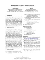
and all share the common problem of needing to estimate the values of a group of parameters. We briefly describe the first three of these systems. In radar we are mterested
in determining the position of an aircraft, as for example, in airport surveillance radar
[Skolnik 1980]. To determine the range R we transmit an electromagnetic pulse that is
reflected by the aircraft, causin an echo to be received b the antenna To seconds later~
as shown in igure 1.1a. The range is determined by the equation TO = 2R/c, where
c is the speed of electromagnetic propagation. Clearly, if the round trip delay To can
be measured, then so can the range. A typical transmit pulse and received waveform
a:e shown in Figure 1.1b. The received echo is decreased in amplitude due to propagatIon losses and hence may be obscured by environmental nois~. Its onset may also be
perturbed by time delays introduced by the electronics of the receiver. Determination
of the round trip delay can therefore require more than just a means of detecting a
jump in the power level at the receiver. It is important to note that a typical modern

l


2

CHAPTER 1. INTRODUCTION

3

1.1. ESTIMATION IN SIGNAL PROCESSING

Sea surface

Transmit/

receive
antenna

Towed array
Sea bottom

'-----+01 Radar processing
system

---------------~~---------------------------~
(a)

(a)

Passive sonar

Radar
Sensor 1 output

Transmit pulse
....................... - - .................... - - ... -1

Time

~
~'C7~

Received waveform

:---- -----_ ... -_ ... _-------,

Time

Time

Sensor 3 output
Time
TO

(b)

~--------- ... ------ .. -- __ ..!

Transmit and received waveforms

Figure 1.1

Radar system

radar s!,stem will input the received continuous-time waveform into a digital computer
by takmg samples via an analog-to-digital convertor. Once the waveform has been
sampled, the data compose a time series. (See also Examples 3.13 and 7.15 for a more
detailed description of this problem and optimal estimation procedures.)
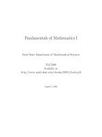
Another common application is in sonar, in which we are also interested in the
posi~ion of a target, such as a submarine [Knight et al. 1981, Burdic 1984] . A typical
passive sonar is shown in Figure 1.2a. The target radiates noise due to machiner:y
on board, propellor action, etc. This noise, which is actually the signal of interest,
propagates through the water and is received by an array of sensors. The sensor outputs

f

~ \~
(b)

/

Time

Received signals at array sensors

Figure 1.2

Passive sonar system

are then transmitted to a tow ship for input to a digital computer. Because of the
positions of the sensors relative to the arrival angle of the target signal, we receive
the signals shown in Figure 1.2b. By measuring TO, the delay between sensors, we can
determine the bearing f3 Z
eTO)
f3 = arccos ( d

(1.1)

where c is the speed of sound in water and d is the distance between sensors (see
Examples 3.15 and 7.17 for a more detailed description). Again, however, the received


CHAPTER 1. INTRODUCTION

4

5

1.1. ESTIMATION IN SIGNAL PROCESSING

S

-.....
<0
-.....
"&

.;,

:s

:~

-.....
<0

-.....

.,u....<0

"C.

"'
u.

p..

0

...:l

-10

"'0

<= -20

-1

:d

S

E

-2
-3
0

2

4

6

8

10

12

14

16

18

20

Time (ms)

-30~

!

!?!' -40-+
!
-0
.;::c -50
p..
0
"

I

S

I

i

500

1000

1500

2000

2500

Frequency (Hz)

::=..

30

tu

10-+

-.....
1
-.....
'" 2°i

<0
::;

C.

U'"

"...:l

0
-10

"2 -20
id
~

-30

I

1

~ -40-+

~ -50il--------~I--------_r1--------TI--------T-------~----

o

8

10

14

0::

0

500

1000

Figure 1.3

Examples of speech sounds

waveforms are not "clean" as shown in Figure 1.2b but are embedded in noise, making,
the determination of To more difficult. The value of (3 obtained from (1.1) is then onli(
an estimate.
- Another application is in speech processing systems [Rabiner and Schafer 1978].
A particularly important problem is speech recognition, which is the recognition of
speech by a machine (digital computer). The simplest example of this is in recognizing
individual speech sounds or phonemes. Phonemes are the vowels, consonants, etc., or
the fundamental sounds of speech. As an example, the vowels /al and /e/ are shown
in Figure 1.3. Note that they are eriodic waveforms whose eriod is called the pitch.
To recognize whether a sound is an la or an lei the following simple strategy might
be employed. Have the person whose speech is to be recognized say each vowel three
times and store the waveforms. To reco nize the s oken vowel com are it to the
stored vowe s and choose the one that is closest to the spoken vowel or the one that

1500

2000

2500

Frequency (Hz)

Time (ms)

Figure 1.4

LPC spectral modeling

minimizes some distance measure. Difficulties arise if the itch of the speaker's voice
c anges from the time he or s e recor s the sounds (the training session) to the time
when the speech recognizer is used. This is a natural variability due to the nature of
human speech. In practice, attributes, other than the waveforms themselves, are used
to measure distance. Attributes are chosen that are less sllsceptible to variation. For
example, the spectral envelope will not change with pitch since the Fourier transform
of a periodic signal is a sampled version of the Fourier transform of one period of the
signal. The period affects only the spacing between frequency samples, not the values.
To extract the s ectral envelo e we em 10 a model of s eech called linear predictive
coding LPC). The parameters of the model determine the s ectral envelope. For the
speec soun SIll 19ure 1.3 the power spectrum (magnitude-squared Fourier transform
divided by the number of time samples) or periodogram and the estimated LPC spectral
envelope are shown in Figure 1.4. (See Examples 3.16 and 7.18 for a description of how


CHAPTER 1. INTRODUCTION

6

the parameters of the model are estimated and used to find the spectral envelope.) It
is interesting that in this example a human interpreter can easily discern the spoken
vowel. The real problem then is to design a machine that is able to do the same. In
the radar/sonar problem a human interpreter would be unable to determine the target
position from the received waveforms, so that the machine acts as an indispensable
tool.
In all these systems we are faced with the problem of extracting values of parameters
bas~ on continuous-time waveforms. Due to the use of di ital com uters to sample
and store e contmuous-time wave orm, we have the equivalent problem of extractin
parameter values from a discrete-time waveform or a data set. at ematically, we have
the N-point data set {x[O], x[I], ... , x[N
which depends on an unknown parameter
(). We wish to determine () based on the data or to define an estimator

-In

1.2. THE MATHEMATICAL ESTIMATION PROBLEM

7

x[O]

Figure 1.5

1.2

Dependence of PDF on unknown parameter

The Mathematical Estimation Problem

In determining good .estimators the first step is to mathematically model the data.

{J = g(x[O] , x[I], . .. , x[N - 1])

(1.2)

where 9 is some function. This is the problem of pammeter estimation, which is the
subject of this book. Although electrical engineers at one time designed systems based
on analog signals and analog circuits, the current and future trend is based on discretetime signals or sequences and digital circuitry. With this transition the estimation
problem has evolved into one of estimating a parameter based on a time series, which
is just a discrete-time process. Furthermore, because the amount of data is necessarily
finite, we are faced with the determination of 9 as in (1.2). Therefore, our problem has
now evolved into one which has a long and glorious history, dating back to Gauss who
in 1795 used least squares data analysis to predict planetary m(Wements [Gauss 1963
(English translation)]. All the theory and techniques of statisti~al estimation are at
our disposal [Cox and Hinkley 1974, Kendall and Stuart 1976-1979, Rao 1973, Zacks
1981].

Before concluding our discussion of application areas we complete the previous list.
4. Image analysis - Elstimate the position and orientation of an object from a camera
image, necessary when using a robot to pick up an object [Jain 1989]
5. Biomedicine - estimate the heart rate of a

fetu~

[Widrow and Stearns 1985]

6. Communications - estimate the carrier frequency of a signal so that the signal can
be demodulated to baseband [Proakis 1983]
1. Control - estimate the position of a powerboat so that corrective navigational
action can be taken, as in a LORAN system [Dabbous 1988]
8. Seismology - estimate the underground distance of an oil deposit based on SOUD&
reflections dueto the different densities of oil and rock layers [Justice 1985].
Finally, the multitude of applications stemming from analysis of data from physical
experiments, economics, etc., should also be mentioned [Box and Jenkins 1970, Holm
and Hovem 1979, Schuster 1898, Taylor 1986].

~ecause the data are mherently random, we describe it by it§, probability density func-

tion (PDF) 01:" p(x[O], x[I], ... , x[N - 1]; ()). The PDF is parameterized by the unknown
l2arameter ()J I.e., we have a class of PDFs where each one is different due to a different
value of (). We will use a semicolon to denote this dependence. As an example, if N = 1
and () denotes the mean, then the PDF of the data might be

p(x[O]; ()) = .:-." exp [__I_(x[O] _
v 27rO' 2

())2]

20'2

which is shown in Figure 1.5 for various values of (). It should be intuitively clear that
because the value of () affects the probability of xiO], we should be able to infer the value
of () from the observed value of x[OL For example, if the value of x[O] is negative, it is
doubtful tha~ () =:' .()2' :rhe value. (). = ()l might be more reasonable, This specification
of th~ PDF IS cntlcal m determmmg a good estima~. In an actual problem we are
not glv~n a PDF but .must choose one that is not only consistent with the problem

~onstramts and any pnor knowledge, but one that is also mathematically tractable. To
~llus~rate the appr~ach consider the hypothetical Dow-Jones industrial average shown
IP. FIgure 1.6. It. mIght be conjectured that this data, although appearing to fluctuate
WIldly, actually IS "on the average" increasing. To determine if this is true we could
assume that the data actually consist of a straight line embedded in random noise or

x[n] =A+Bn+w[n]

n = 0, 1, ... ,N - 1.

~ reasonable model for the noise is that win] is white Gaussian noise (WGN) or each
sample of win] has the PDF N(0,O' 2 ) (denotes a Gaussian distribution with a mean
of 0 and a variance of 0'2) and is uncorrelated with all the other samples. Then, the
unknown parameters are A and B, which arranged as a vector become the vector
parameter 9 = [A Bf. Letting x = [x[O] x[I] . .. x[N - lW, the PDF is
p(x; 9)

1 [1

= (27rO'2)~

N-l

]

exp - 20'2 ~ (x[n]- A - Bn)2 .

(1.3)

The choice of a straight line for the signal component is consistent with the knowledge

that the Dow-Jones average is hovering around 3000 (A models this) and the conjecture


8

CHAPTER 1. INTRODUCTION
3200

3.0

3150

2.5-+

~

3100

~

"
"0
.-,

3050

'Il

3000

...<'$
~

~0

0

1.3. ASSESSING ESTIMATOR PERFORMANCE

"F.
fl

9

i

1.0

0.5
0.0

2950

-{)'5~

2900

-1.0

2850

-1.5

2800
0

10

20

30

40

50

60

70

80

90

- 2 . 0 - r - - ' I - - i l - - i l - - i l - - i l - - I I - - I I_ _"1'I_ _-+1----<1

100

o

ill

W

~

~

Day number

Figure 1.6 Hypothetical Dow-Jones average

that it is increasing (B > 0 models this). The assumption of WGN is justified by the
need to formulate a mathematically tractable model so that closed form estimators can
be found. Also, it is reasonable unless there is strong evidence to the contrary, such as
highly correlated noise. Of course, the performance of any estimator obtained will be
critically dependent on the PDF assum tions. We can onl hope the estimator obtained
is robust, in that slight changes in the PDF do not severely affect t per ormance of the
estimator. More conservative approaches utilize robust statistical procedures [Huber
1981J.
Estimation based on PDFs such as (1.3) is termed classical estimation in that the
parameters of interest are assumed to be deterministic but unknown. In the Dow-Jo~
average example we know a priori that the mean is somewhere around 3000. It seems
inconsistent with reality, then, to choose an estimator of A that can result in values as
low as 2000 or as high as 4000. We might be more willing to constrain the estimator
to produce values of A in the range [2800, 3200J. To incorporate this prior knowledge
we can assume that A is no Ion er deterministic but a random variable and assign it a
DF, possibly uni orm over the [2800, 3200J interval. Then, any subsequent estImator
will yield values in this range. Such an approach is termed Bayesian estimation. The
parameter we are attem tin to estimate is then viewed as a realization of the randQ;

, the data are described by the joint PDF

p(x,9)

= p(xI9)p(9)

M

W

m

W

00

~

n

Figure 1. 7

Realization of DC level in noise

Once
the PDF has been
specified the problem becomes one 0 f d et ermmmg
..
"
. '

an
optImal estImator or functlOn of the data ' as in (1 .2) . Note that an es t'Imat or may
depend on other par~meters, but only if they are known. An estimator may be thought
of as a rule that ~Sl ns a value to 9 for each realization of x. The estimate of 9 is
the va ue o. 9 obtal~ed .for a given realization of x. This distinction is analogous to a
random vanable (whIch IS a f~nction defined on the sample space) and the value it takes
on. Althoug~ some authors dIstinguish between the two by using capital and lowercase
letters, we WIll not do so. The meaning will, hopefully, be clear from the context.

1.3

Assessing Estimator Performance

Consider. the data set shown in Figure 1.7. From a cursory inspection it appears that

x[n] conslst~ of.a DC.level A in noise. (The use of the term DC is in reference to direct
current, whIch IS eqUlvalent to the constant function.) We could model the data as

x[nJ

= A + wIn]

;~re w n denotes so~e zero ~ean noise ro~~ss. B~ed on the data set {x[O], x[1], .. . ,
[[ .l]), we would .hke to estImate A. IntUltlvely, smce A is the average level of x[nJ
(w nJ IS zero mean), It would be reasonable to estimate A as
I

.4= N

N-l

Lx[nJ
n=O

or by the sample mean of the data. Several questions come to mind:

I 1. How close will .4 be to A?

'\ 2. Are there better estimators than the sample mean?


10

CHAPTER 1. INTRODUCTION

For the data set in Figure 1.7 it turns out that
of A = 1. Another estimator might be

1.3. ASSESSING ESTIMATOR PERFORMANCE

.1= 0.9, which is close to the true value

A=x[o].
Intuitively, we would not expect this estimator to perform as well since it does not
make use of all the data. There is no averaging to reduce the noise effects. However,
for the data set in Figure 1.7, A = 0.95, which is closer to the true value of A than
the sample mean estimate. Can we conclude that A is a better estimator than A?
The answer is of course no. Because an estimator is a function of the data, which
are random variables, it too is a random variable, subject to many possible outcomes.
The fact that A is closer to the true value only means that for the given realization of

data, as shown in Figure 1.7, the estimate A = 0.95 (or realization of A) is closer to
the true value than the estimate .1= 0.9 (or realization of A). To assess performance
we must do so statistically. One possibility would be to repeat the experiment that
generated the data and apply each estimator to every data set. Then, we could ask
which estimator produces a better estimate in the majority of the cases. Suppose we
repeat the experiment by fixing A = 1 and adding different noise realizations of win] to
generate an ensemble of realizations of x[n]. Then, we determine the values of the two
estimators for each data set and finally plot the histograms. (A histogram describes the
number of times the estimator produces a given range of values and is an approximation
to the PDF.) For 100 realizations the histograms are shown in Figure 1.8. It should
now be evident that A is a better estimator than A because the values obtained are
more concentrated about the true value of A = 1. Hence, A will uliWl-lly produce a value
closer to the true one than A. The skeptic, however, might argue-that if we repeat the
experiment 1000 times instead, then the histogram of A will be more concentrated. To
dispel this notion, we cannot repeat the experiment 1000 times, for surely the skeptic
would then reassert his or her conjecture for 10,000 experiments. To prove that A is
better we could establish that the variance is less. The modeling assumptions that we
must employ are that the w[n]'s, in addition to being zero mean, are uncorrelated and
have equal variance u 2 . Then, we first show that the mean of each estimator is the true
value or

30

r

'" 25j

1j
20

'0

15

lil

r:~i
-3

~JI~m

------rl- r - I------;--------1
-2
-1
0

=

1
N

'I

i
I

o

-1

2

First sample value,

Figure 1.8

1

N2

N-l

L

var(x[nJ)

n=O

L E(x[n])

1
2
Nu
N2
u2
N

since the w[nJ's are uncorrelated and thus

so that on the average the estimators produce the true value. Second, the variances are

var(A)

=

)
1 N-l
var ( N ~ x[nJ

3

A

Histograms for sample mean and first sample estimator

N-l

A
E(x[O])
A

A

1

n=O

E(A)

---r---I_
2

Sample mean value,

1 N-l
)
E ( N ~ x[nJ

E(A)

11

var(A)

var(x[OJ)
u2
> var(A).

~


12

CHAPTER 1. INTRODUCTION

Furthermore, if we could assume that w[n] is Gaussian, we could also conclude that the
probability of a given magnitude error is less for A. than for A (see Problem 2.7).
ISeveral important points are illustrated by the previous example, which should
always be ept in mind.
1. An estimator is a random variable. As such, its
pletely descri e statistical y or by its PDF.

erformance can onl be com-

2. The use of computer simulations for assessing estimation performance, although
quite valuable for gaiiiing insight and motivating conjectures, is never conclusive.
At best, the true performance may be obtained to the desired degree of accuracy.
At worst, for an insufficient number of experiments and/or errors in the simulation
techniques employed, erroneous results may be obtained (see Appendix 7A for a
further discussion of Monte Carlo computer techniques).
Another theme that we will repeatedly encounter is the tradeoff between perfor:
mance and computational complexity. As in the previous example, even though A
has better performance, it also requires more computation. We will see that QPtimal
estimators can sometimes be difficult to implement, requiring a multidimensional optimization or inte ration. In these situations, alternative estimators that are suboptimal,
but which can be implemented on a igita computer, may be preferred. For any particular application, the user must determine whether the loss in performance is offset
by the reduced computational complexity of a suboptimal estimator.

1.4

Some Notes to the Reader

Our philosophy in presenting a theory of estimation is to provide the user with the
main ideas necessary for determining optimal estimator.§. We have included results
that we deem to be most useful in practice, omitting some important theoretical issues.
The latter can be found in many books on statistical estimation theory which have
been written from a more theoretical viewpoint [Cox and Hinkley 1974, Kendall and
Stuart 1976--1979, Rao 1973, Zacks 1981]. As mentioned previously, our goal is t<;)
obtain an 0 timal estimator, and we resort to a subo timal one if the former cannot
be found or is not implement a ~. The sequence of chapters in this book follows this
approach, so that optimal estimators are discussed first, followed by approximately
optimal estimators, and finally suboptimal estimators. In Chapter 14 a "road map" for

finding a good estimator is presented along with a summary of the various estimators
and their properties. The reader may wish to read this chapter first to obtain an
overview.
We have tried to maximize insight by including many examples and minimizing
long mathematical expositions, although much of the tedious algebra and proofs have
been included as appendices. The DC level in noise described earlier will serve as a
standard example in introducing almost all the estimation approaches. It is hoped
that in doing so the reader will be able to develop his or her own intuition by building
upon previously assimilated concepts. Also, where possible, the scalar estimator is

REFERENCES

13

presented first followed by the vector estimator. This approach reduces the tendency
of vector/matrix algebra to obscure the main ideas. Finally, classical estimation is
described first, followed by Bayesian estimation, again in the interest of not obscuring
the main issues. The estimators obtained using the two approaches, although similar
in appearance, are fundamentally different.
The mathematical notation for all common symbols is summarized in Appendix 2.
The distinction between a continuous-time waveform and a discrete-time waveform or
sequence is made through the symbolism x(t) for continuous-time and x[n] for discretetime. Plots of x[n], however, appear continuous in time, the points having been connected by straight lines for easier viewing. All vectors and matrices are boldface with
all vectors being column vectors. All other symbolism is defined within the context of
the discussion.

References
Box, G.E.P., G.M. Jenkins, Time Series Analysis: Forecasting and Contro~ Holden-Day, San
Francisco, 1970.
Burdic, W.S., Underwater Acoustic System Analysis, Prentice-Hall, Englewood Cliffs, N.J., 1984.
Cox, D.R., D.V. Hinkley, Theoretical Statistics, Chapman and Hall, New York, 1974.

Dabbous, T.E., N.U. Ahmed. J.C. McMillan, D.F. Liang, "Filtering of Discontinuous Processes
Arising in Marine Integrated Navigation," IEEE Trans. Aerosp. Electron. Syst., Vol. 24,
pp. 85-100, 1988.
Gauss, K.G., Theory of Motion of Heavenly Bodies, Dover, New York, 1963.
Holm, S., J.M. Hovem, "Estimation of Scalar Ocean Wave Spectra by the Maximum Entropy
Method," IEEE J. Ocean Eng., Vol. 4, pp. 76-83, 1979.
Huber, P.J., Robust Statistics, J. Wiley, ~ew York, 1981.
Jain, A.K., Fundamentals of Digital Image ProceSSing, Prentice-Hall, Englewood Cliffs, N.J., 1989.
Justice, J.H .. "Array Processing in Exploration Seismology," in Array Signal Processing, S. Haykin,
ed., Prentice-HaU, Englewood Cliffs, N.J., 1985.
Kendall, Sir M., A. Stuart, The Advanced Theory of Statistics, Vols. 1-3, Macmillan, New York,
1976--1979.
Knight, W.S., RG. Pridham, S.M. Kay, "Digital Signal Processing for Sonar," Proc. IEEE, Vol.
69, pp. 1451-1506. Nov. 1981.
Proakis, J.G., Digital Communications, McGraw-Hill, New York, 1983.
Rabiner, L.R., RW. Schafer, Digital Processing of Speech Signals, Prentice-Hall, Englewood Cliffs,
N.J., 1978.

Rao, C.R, Linear Statistical Inference and Its Applications, J. Wiley, New York, 1973.
Schuster, !," "On the Investigation of Hidden Periodicities with Application to a Supposed 26 Day
. PerIod of Meterological Phenomena," Terrestrial Magnetism, Vol. 3, pp. 13-41, March 1898.
Skolmk, M.L, Introduction to Radar Systems, McGraw-Hill, ~ew York, 1980.
Taylor, S., Modeling Financial Time Series, J. Wiley, New York, 1986.
Widrow, B., Stearns, S.D., Adaptive Signal Processing, Prentice-Hall, Englewood Cliffs, N.J., 1985.
Zacks, S., Parametric Statistical Inference, Pergamon, New York, 1981.


CHAPTER 1. INTRODUCTION

14

Problems
1. In a radar system an estimator of round trip delay To has the PDF To ~ N(To, (J~a)"
where 7< is the true value. If the range is to be estimated, propose an estimator R
and find its PDF. Next determine the standard deviation (J-ra so that 99% of th~
time the range estimate will be within 100 m of the true value. Use c = 3 x 10
mls for the speed of electromagnetic propagation.

2. An unknown parameter fJ influences the outcome of an experiment which is modeled by the random variable x. The PDF of x is
p(x; fJ)

=

vk

exp

[-~(X - fJ?) .

A series of experiments is performed, and x is found to always be in the interval
[97, 103]. As a result, the investigator concludes that fJ must have been 100. Is
this assertion correct?
3. Let x = fJ + w, where w is a random variable with PDF Pw( w) ..IfbfJ is (a dfJet)er~in~
istic parameter, find the PDF of x in terms of pw and denote It y P x; ... ex
assume that fJ is a random variable independent of wand find the condltlO?al
PDF p(xlfJ). Finally, do not assume that eand ware independent and determme
p(xlfJ). What can you say about p(x; fJ) versus p(xlfJ)?
4. It is desired to estimate the value of a DC level A in WGN or

x[n] = A + w[n]

n

= 0,1, ... , N

-

C

where w[n] is zero mean and uncorrelated, and each sample has variance
Consider the two estimators
1 N-I
A = N
x[n]

(J2

=

l.

2::

n=O

A

_1_ (2X[0]

N

+2

+ ~ x[n] + 2x[N -

1]) .

n=1

Which one is better? Does it depend on the value of A?
5. For the same data set as in Problem 1.4 the following estimator is proposed:
x [0]

A= {

~'~x[n]

A2
.,.2

= A2 < 1000 .
-

The rationale for this estimator is that for a high enough signal-to-noise ratio
(SNR) or A2/(J2, we do not need to reduce the effect of.noise by averaging and
hence can avoid the added computation. Comment on thiS approach.

Chapter 2

Minimum Variance Unbiased

Estimation

2.1

Introduction

In this chapter we will be in our search for good estimators of unknown deterministic
parame ers.
e will restrict our attention to estimators which on the average yield
the true parameter value. Then, within this class of estimators the goal will be to find
the one that exhibits the least variability. Hopefully, the estimator thus obtained will
produce values close to the true value most of the time. The notion of a minimum
variance unbiased estimator is examined within this chapter, but the means to find it
will require some more theory. Succeeding chapters will provide that theory as well as
apply it to many of the typical problems encountered in signal processing.

2.2

Summary

An unbiased estimator is defined by (2.1), with the important proviso that this holds for
all possible values of the unknown parameter. Within this class of estimators the one
with the minimum variance is sought. The unbiased constraint is shown by example
to be desirable from a practical viewpoint since the more natural error criterion, the
minimum mean square error, defined in (2.5), generally leads to unrealizable estimators.
Minimum variance unbiased estimators do not, in eneral, exist. When they do, several
methods can be used to find them. The methods reI on the Cramer-Rao ower oun
and the concept of a sufficient statistic. If a minimum variance unbiase estimator
does not exist or if both of the previous two approaches fail, a further constraint on the
estimator, to being linear in the data, leads to an easily implemented, but suboptimal,

estimato!,;

15


CHAPTER 2. MINIMUM VARIANCE UNBIASED ESTIMATION

16

2.3

2.3. UNBIASED ESTIMATORS

17

Unbiased Estimators

For an estimator to be unbiased we mean that on the average the estimator will yield
the true value of the unknown parameter. Since the parameter value may in general be
anywhere in the interval a < 8 < b, unbiasedness asserts that no matter what the true
value of 8, our estimator will yield it on the average. Mathematically, an estimator i~
~~~il

•

A

E(iJ) = 8

(2.1)

Figure 2.1

where (a,b) denotes the range of possible values of 8.

Example 2.1 - Unbiased Estimator for DC Level in White Gaussian Noise

Probability density function for sample mean estimator

It is possible, however, that (2.3) may hold for some values of 8 and not others as the
next example illustrates.
'

Consider the observatioJ!s

x[n) = A + w[n)

Example 2.2 - Biased Estimator for DC Level in White Noise

n = 0, 1, ... ,N - 1

where A is the parameter to be estimated and w[n] is WGN. The parameter A can
take on any value in the interval -00 < A < 00. Then, a reasonable estimator for the
average value of x[n] is

Consider again Example 2.1 but with the modified sample mean estimator
_

1

N-1

A= 2N Lx[n].
(2.2)

Then,

or the sample mean. Due to the linearity properties of the expectation operator

E(A.)

=

E(x[nJ)

It is seen that (2.3) holds for the modified estimator only for A =
biased estimator.

n=O
N-1

~LA
n=O
=

A

for all A. The sample mean estimator is therefore unbiased.

<>

In this example A can take on any value, although in general the values of an unknown
parameter may be restricted by physical considerations. Estimating the resistance R
of an unknown resistor, for example, would necessitate an interval 0 < R < 00.
Unbiased estimators tend to have symmetric PDFs centered about the true value of
8, although this is not necessary (see Problem 2.5). For Example 2.1 the PDF is shown
in Figure 2.1 and is easily shown to be N(A, (72/N) (see Problem 2.3).
The restriction that E(iJ) = 8 for all 8 is an important one. Lettin iJ =
x = [x 0 x
, it asserts that

E(iJ) =

J

g(x)p(x; 8) dx = 8

2
A if A=O
A if A # o.

#

N-1

L

~A

E(A)

]
1 N-1
E [ N ~ x[n)

1
N

n=O

for all 8.

(2.3)

o.

Clearly,

A is

a

<>

That an estimator is unbiased does not necessarily mean that it is a good estimator.
It only guarantees that on the average it will attain the true value. On the other hand
biased estimators are ones that are characterized by a systematic error, which presum~
ably should not be present. A persistent bias will always result in a poor estimator.
As an example, the unbiased property has an important implication when several estimators are combined (see Problem 2.4). ~t s?metimes occurs that multiple estimates
~th~ same paran:eter ar.e available, i.e., {81 , 82 , •.. , 8n }. A reasonable procedure is to
combme these estimates mto, hopefully, a better one by averaging them to form

.

1 ~.

8=- ~8i.
n

(2.4)

i=l

Assuming the estimators are unbiased, with the same variance, and uncorrelated with
each other,

E(iJ)

=8


X[~] ~ N (f)/ 1 )

X [1\] -'?-

\ f'I C~, 1)

tt;:; [~1 ~2 ~ - - &p 1

, &;; 0 I

') N (f), 2) ) 9-.( 0 (

~ [X [, 1 + x[l]
'2

i1"

O

!..

2 > q,

f.

(~);:

@'1'

~=----[9~~~.~ Sp]"

)

.•

_-_........

I

_.

..

('2. Xfr,J + X[11)

Qi 1.
'

~. < ('9t.
1

D

GJ-~')~

'- tlt¥;

1"

ry

J -L i

I

-=>

£. p

t

------:;-----====--

-.-----:-===:====---:::::--~-...

0:

~ e, l : r 1I (!. ~~, _J.!.1'" *
~i
l \;!
,". [J

0'"" J :,

-I

f

'\"

~

'>1

'v

(

"'A

)"7.

'\ ")2 .\
~@(
-=., i ~i
~

" 1:

-

'
~

;, -;- t
IV

.\(}oJ
A)1
"[: @,:
,. I

~-

Q.

-::;

N

(

-t

/VZ

~~

~
9.
1~'
IJ

J~
L~(
I
)/'J
1

.f C

1:"

E.

)

.J

'''-'

-1

,tl

L
,-.,
IV

~

Z.

Ju

~ Z~ &i'" ~ . ("'t --1 :c 9i 1

E

!:'

H

J
k < (-' :r &; - ~ ?: t\ .1 1;
N ,=,
tV '>1
tJ

,1

A
Z= -r
1)1

N'

J

i- - ;

IJ

to

1?:~ Sr:~ ~I-.
,.,

~t 1(L" e ~ E [~
f\I

;.,

A

\ _

i

I

).

JJ ;

,
~ ~~9~~: _t f-\(e~ -E~e~\n ; t(l;~e/ ~ _E1 S ~ 2)

q

~I

,., .... I

.. -.~~

1

.=:

i

I

i; ~~6/\(..(li~/~ E~ t~~i~ f~~J' 1?~i t~914
/

~

')

tl"~ \tt~&.~ i~-ks 1~ 0; ~ ~ ~ ~
--J>

C

&j

"t, { G 1

~_


CHAPTER 2. MINIMUM VARIANCE UNBIASED ESTIMATION

18

19

2.4. MINIMUM VARIANCE CRITERION

2.4

Minimum Variance Criterion

p(8)

In searching for optimal estimators we need to ado t some

natura one is the mean square error (MSE), defined as

n increases
~

__+-____ __ __
~

~

~~

0

____ O

(2.5)

IJ

(a)

Unbiased estimator

This measures the avera e mean s uared deviation of the estimator from the t e value.
Unfortunate y, adoption of this natural criterion leads to unrealizable estimators ones
that cannot be written solely as a function of the data. To understand the pr~blem
which arises we first rewrite the MSE as

p(O)

mse(8)

..

=

E{[(8-E(O))+(E(O)-8)f}

n increases

__~~--~--~~-------O
E(9)

__+-_'-...,.---'..,.....--------- 0

IJ

(b)

Figure 2.2

Biased estimator

Effect of combining estimators

+ [E(8) var(8) + b2 (8)
var(O)

8f

(2.6)

which shows that the MSE is composed of errors due to the variance of the estimator as
well as the bias. As an example, for the problem in Example 2.1 consider the modified
estimator
.
1 N-l

A=a

N

Lx[nj
n=O

for some c:onstant a. We wi~l attempt to find the a which results in the minimum MSE.
Since E(A) = aA and var(A) = a2(j2/N, we have, from (2.6),

and

=

var(8d
n

Differentiating the MSE with respect to a yields

so that as more estimates are averaged, the variance will decrease. Ultimately, as
n -+ 0Cl, {} -+ 8. However, if the estimators are biased or E(8 i ) = 8 + b(8), then

dmse(A)
2a(j2
da
=N

+ 2(a -

2

l)A

which upon setting to zero and solving yields the optimum value
8 + b(8)

and no matter how many estimators are avera ed 8 will not conver e to the true value.
This is depicted in igure 2.2. Note that, in general,

b(8)
is defined as the bias of the estimator.

= E(8) -

8

a

A2

- -------

opt -

A2

+ (j2/N'

It is seen that, unfortunately, the optimal value of a depends upon the unknown parameter A. ~he estimator is therefore not realizable. In retrospect the estimator depends
up~n A smce the bias ter~ in ~2.6) is a function of A. It would seem that any criterion
which depends on the bias Will lead to an unrealizable estimator. Although this is
gene~~lly true, on occasion realizable minimum MSE estimators can be found [Bibby
and Ioutenburg 1977, Rao 1973, Stoica and Moses 1990j.


20

CHAPTER 2. MINIMUM VARIANCE UNBIASED ESTIMATION

2.6.

var(ii)

var(8)

var(8)

_

-+-----

-4--------

-1_ _ _ _ _---

iii

_+-__-----

2

8

83 = MVU estimator

-

82
03

•••••••••.••.•.•••• ·2·ciiji

NoMVU
estimator

27 36
/

01

18/36

__---------t---------------

90

Possible dependence of estimator variance with

Figure 2.4 Illustration of nonexistence of minimum variance unbiased estimator

The two estimators

(J

1

- (x[Q]
2

From a practical view oint the minimum MSE estimator needs to be abandoned.
An alternative approach is to constrain t e bias to be zero and find the estimator which
minimizes the variance. Such an estimator is termed the minimum variance unbiased
(MVU) estimator. Note that from (2.6) that the MSE of an unbiased estimator is just
the variance.
Minimizing the variance of an unbiased estimator also has the effect of concentrating
the PDF of the estimation error, 0 - B, about zero (see Problem 2.7). The estimatiw
error Will therefore be less likely to be large.

2.5

9

(b)

(a)
Figure 2.3

-

_------"1 :~!~?.................. ii2

81

--+-----~~----------- 9

--~------------------- 9

21

FINDING THE MVU ESTIMATOR

2
3

-x[Q]

+ x[l])
1
3

+ -x[l]

can easily be shown to be unbiased. To compute the variances we have that
1
- (var(x[O])
4

4
-var(x[O])

9

+ var(x[l]))

1
+ -var(x[l])

9

so that

Existence of the Minimum Variance Unbiased
Estimator

The uestion arises as to whether a MVU estimator exists Le., an unbiased estimator
wit minimum variance for all B. Two possible situations are describe in Figure ..
If there are three unbiased estimators that exist and whose variances are shown in
Figure 2.3a, then clearly 03 is the MVU estimator. If the situation in Figure 2.3b
exists, however, then there is no MVU estimator since for B < Bo, O2 is better, while
for iJ > Bo, 03 is better. In the former case 03 is sometimes referred to as the uniformly
minimum variance unbiased estimator to emphasize that the variance is smallest for
all B. In general, the MVU estimator does not always exist, as the following example

illustrates.
.

and

¥s

if B < O.

The variances are shown in Figure 2.4. Clearly, between these two esti~~tors no M:'U
estimator exists. It is shown in Problem 3.6 that for B ~ 0 the mInimum possible
variance of an unbiased estimator is 18/36, while that for B < 0 is 24/36. Hence, no
single estimator can have a variance uniformly less than or equal to the minima shown
in Figure 2.4.
0

Example 2.3 - Counterexample to Existence of MVU Estimator

To conclude our discussion of existence we should note that it is also possible that there
may not exist even a single unbiased estima.!2E (see Problem 2.11). In this case any
search for a MVU estimator is fruitless.

If the form ofthe PDF changes with B, then it would be expected that the best estimator
would also change with B. Assume that we have two independent observations x[Q] and
x[l] with PDF

2.6

x [0]

x[l]

N(B,l)
N(B,l)
{ N(B,2)

is no known
Even if a MVU estimator exists, we may not be able to find it.
urn-t e-crank" procedure which will always produce the estimator. In the next few
chapters we shall discuss several possible approaches. They are:

if B ~ Q
if B < O.

••7F."'F'~· __ · _ _
' ' ' ' '. . . . ._ _ _ _-

Finding the Minimum Variance
Unbiased Estimator

:"'$

_ _


22

CHAPTER 2. MINIMUM VARIANCE UNBIASED ESTIMATION

23

REFERENCES
var(O)

we can equivalently define an unbiased estimator to have the property
E(8)

............ ••••••••••••••• ····CRLB

----------------r-------------------- 9

Figure 2.5 Cramer-Rao
lower bound on variance of unbiased
estimator

1. Determine the Cramer-Rao lower bound CRLB and check to see if some estimator
satisfies it Chapters 3 and 4).

2. Apply the Rao-Blackwell-Lehmann-Scheffe (RBLS) theorem (Chapter 5).
3. Further restrict the class of estimators to be not only unbiased but also linear. Then,
find the minimum variance estimator within this restricted class (Chapte~ 6).

Approaches 1 and 2 may produce the MVU estimator, while 3 will yield it only if the
MVU estimator is linear III the data.
The CRLB allows us to determine that for any unbiased estimator the variance
must be greater than or equal to a given value, as shown in Figure 2.5. If an estimator
exists whose variance equals the CRLB for each value of (), then it must be the MVU
estimator. In this case, the theory of the CRLB immediately yields the estimator. It
may happen that no estimator exists whose variance equals the bound. Yet, a MV~
estimator may still exist, as for instance in the case of ()! in Figure 2.5. Then, we

must resort to the Rao-Blackwell-Lehmann-Scheffe theorem. Thts procedure first find;
a su czen s atistic, one whic uses a the data efficient! and then nds a unction
of the su dent statistic which is an unbiased estimator oL(}. With a slight restriction
of the PDF of the data this procedure will then be guaranteed to produce the MVU
estimator. The third approach requires the estimator to be linear, a sometimes severe
restriction, and chooses the best linear estimator. Of course, only for particular data
sets can this approach produce the MVU estimator.

.

2. 7

Extension to a Vector Parameter

,

A

A

ai

for i

= 1,2, ... ,p.

<

(}i

< b;

for every 8 contained wjthjn the space defined in (2.7). A MVU estimator has the
~ditional property that var(Bi) for i = 1,2, ... ,p is minimum among all unbiased
estimators.

References
Bibbv, J .. H. Toutenburg, Prediction and Improved Estimation in Linear Models, J. Wiley, New
. York, 1977.
Rao, C.R., Linear Statistical Inference and Its Applications, J. Wiley, New York, 1973.
Stoica, P., R. Moses, "On Biased Estimators and the Unbiased Cramer-Rao Lower Bound," Signal
Process., Vol. 21, pp. 349-350, 1990.

Problems
2.1 The data {x[O], x[I], ... ,x[N - I]} are observed where the x[n]'s are independent
and identically distributed (lID) as N(0,a 2 ). We wish to estimate the variance
a 2 as

Is this an unbiased estimator? Find the variance of ;2 and examine what happens
as N -t 00.
2.2 Consider the data {x[O],x[I], ... ,x[N -l]}, where each sample is distributed as
U[O, ()] and the samples are lID. Can you find an unbiased estimator for ()? The
range of () is 0 < () < 00.
2.3 Prove that the PDF of

If 8 = [(}l (}2 •.. (}"jT is a vector of unknown parameter~, then we say that an estimator
'T
•
8 = [(}1 (}2 •.• (},,] is unbiase~j,f
(2.7)

=8

A given in Example 2.1

is N(A, a 2 IN).

2.4 The heart rate h of a patient is automatically recorded by a computer every 100 ms.
In 1 s the measurements {hI, h2 , ••• , hlO } are averaged to obtain h. If E(h;) = ah
for some constant a and var(h i ) = 1 for each i, determine whether averaging
improves the estimator if a = 1 and a = 1/2. Assume each measurement is
uncorrelated.

By defining
2.5 Two samples {x [0], x[l]} are independently observed from a N(O, a 2 ) distribution.
The estimator
1
a 2 = 2'(x 2 [0] + x 2 [1])
A

is unbiased. Find the PDF of ;2 to determine if it is symmetric about a 2 •


24

CHAPTER 2. MINIMUM VARIANCE UNBIASED ESTIMATION

. gI bservation x[O] from the distribution Ufo, 1/(}], it is desired to
2.11 estimate
Given a ().

sm rt e.IS0 assume d that () > O. Show that for an estimator 0 = g(x[O]) to

.v-I

A=

L

anx[n]

be unbiased we must have

n=O

is proposed. Find the an's so that the estimator is unbiased and the variance is
minimized. Hint: Use Lagrangian mUltipliers with unbiasedness as the constraint
equation.

2.7 Two unbiased estimators are proposed whose variances satisfy var(O) < var(B). If
both estimators are Gaussian, prove that

f:

for any > O. This says that the estimator with less variance is to be preferred
since its PDF is more concentrated about the true value.

2.8 For the problem described in Example 2.1 show that as N -t
the results of Problem 2.3. To do so prove that
lim Pr {IA

N-+oo

00,

A -t A

by using

- AI> f:} = 0

f:

for any > O. In this case the estimator
what happens if the alternative estimator

A is said

to be consistent. Investigate

A = 2~ L::OI x[n] is used instead.

2.9 This problem illustrates what happens to an unbiased est!1nator when it undergoes
a nonlinear transformation. In Example 2.1, if we choose to estimate the unknown
parameter () = A 2 by

0=

(~ ~Ix[n]r,

can we say that the estimator is unbiased? What happens as N -t oo?

2.10 In Example 2.1 assume now that in addition to A, the value of 172 is also unknown.
We wish to estimate the vector parameter

Is the estimator
N1 N-I
Lx[n]

[,;, 1~ ~ ~
,

A

[ N

unbiased?

]

n=O

1

(x[n] -

A)'

25

PROBLEMS

2.6 For the problem described in Example 2.1 the more general estimator

1#

g(u)du = l.

Next. prove that a function 9 cannot be found to satisfy this condition for all () > O.


Chapter 3

Cramer-Rao Lower Bound
3.1

Introduction

Being able to place a lower bound on the variance of any unbiased estimator proves
to be extremely useful in practice. At best, it allows us to assert that an estimator is
the MVU estimator. This will be the case if the estimator attains the bound for all
values of the unknown parameter. At worst, it provides a benchmark against which we
can compare the performance of any unbiased estimator. Furthermore, it alerts us to
the physical impossibility of finding an unbiased estimator whose variance is less than
the bound. The latter is often useful in signal processing feasibility studies. Although
many such variance bounds exist [McAulay and Hofstetter 1971, Kendall and Stuart
1979, Seidman 1970, Ziv and Zakai 1969], the Cramer-Rao lower bound (CRLB) is by
far the easiest to determine. Also, the theory allows us to immediately determine if
an estimator exists that attains the bound. If no such estimator exists, then all is not
lost since estimators can be found that attain the bound in an approximate sense, as
described in Chapter 7. For these reasons we restrict our discussion to the CRLB.

3.2

Summary

The CRLB for a scalar parameter is given by (3.6). If the condition (3.7) is satisfied,
then the bound will be attained and the estimator that attains it is readily found.
An alternative means of determining the CRLB is given by (3.12). For a signal with
an unknown parameter in WGN, (3.14) provides a convenient means to evaluate the
bound. When a function of a parameter is to be estimated, the CRLB is given by
(3.16). Even though an efficient estimator may exist for (), in general there will not be
one for a function of () (unless the function is linear). For a vector parameter the CRLB
is determined using (3.20) and (3.21). As in the scalar parameter case, if condition
(3.25) holds, then the bound is attained and the estimator that attains the bound is
easily found. For a function of a vector parameter (3.30) provides the bound. A general
formula for the Fisher information matrix (used to determine the vector CRLB) for a
multivariate Gaussian PDF is given by (3.31). Finally, if the data set comes from a
27


CHAPTER 3. CRAMER-RAO LOWER BOUND

3.3. ESTIMATOR ACCURACY CONSIDERATIONS

29

this we determine the probability of observing x[O] in the interval [ [ ][3 _ J/2, 3 + J/2] when A takes on a given value or
x 0 J/2, x[0]+J/2]

=

28
PI (x [0]

p2(X[0] = 3; A)

= 3; A)

{ J

J} =

Pr 3 - 2" :::; x[O] :::; 3 + 2"

__r--r__~-r--~-r--r-------2

3

4

(a)

5
<11

23456

= 1/3

(b)

<12

= 1

PDF dependence on unknown parameter

WSS Gaussian random process, then an approximate CRLB, that depends on the PSD,
is given by (3.34). It is valid asymptotically or as the data record length becomes large.

3.3

Estimator Accuracy Considerations

Before stating the CRLB theorem, it is worthwhile to expose the hidden factors that
determine how well we can estimate a parameter. Since all our information is embodied
in the observed data and the underlying PDF for that data it is not sur risin that the
estimation accuracy depen s uect Y on the PDF. For instance, we should not expect
to be able to estimate a parameter with any degree of accuracy if the PDF depends
only weakly upon that parameter, or in the extreme case, i!.the PDF does not depend
on it at all. In general, the more the PDF is influenced by the unknown parameter, the
better we shou

2

A

6

Figure 3.1

r3+~

J3-~ Pi(U; A) du

e a e to estimate it.

l~

which for J small is Pi (x[O] = 3; A)J. But PI (x[O] = 3' A = 4)J .
3; A = 3)J = 1.20J. The probability of observing x[O] 'in a
O.OlJ, while PI (x [0] =
x[O] = 3 when A = 4 is small with respect to that h
~nterval centered about
A > 4 can be eliminated from consideration. It mthte~ - . Hence, the values ?f
the interval 3 ± 3a l = [2,4] are viable candidates
values of A III
is a much weaker dependence on A. Here our . b'l
d' d
Fill. Figure 3.1 b there
via e can I ates are III the much wider
interval 3 ± 3a2 = [0,6].

S;=-

~or t~ea~~ed. tha~

o

When the PDF is viewed as a function of th

k
it is termed the likelihood function. Two exam l:su~f ~~w~ paramete: (with x fixed),
in Figure 3.1. Intuitively, the "sharpness" of &e likelih~h~o~d fu.nctlOns we:e shown
we can estimate the unknown paramet er T0 quantify
0
unctIOn
accurately
ha h
thi determllles
f
b how
. .
s no Ion 0 serve
t t t e sharpness is effectively measured b th
the logarithm of the likelihood function at i~s :a~eg;t~~e .of the second derivative of
1 if we cons I.Pd er t·h e natural
IS IS the
curvature
loglikelihood function. In Example 3.,
logarithm
of of
thethe
PDF
Inp(x[O]; A) = -In v'21ra 2

_l_(x[O]_
A)2
2a 2

then the first derivative is

81np(x[0]; A)

Example 3.1 _ PDF Dependence on Unknown Parameter

-

8A

1

= 0-2 (x[O]

- A)

(3.2)

and the negative of the second derivative becomes

If a single sample is observed as

x[O]

_ 8 2 1np(x[0];A)
1
8A2
-a 2 '

= A + w[O]

where w[O] '" N(O, 0-2 ), and it is desired to estimate A, then we expect a better estimate

if 0-2 is small. Indeed, a good unbiased estimator is A. = x[O]. The variance is, of course,
2
just 0-2, so that the estimator accuracy improves as 0- decreases. An alternative way
of viewing this is shown in Figure 3.1, where the PDFs for two different variances are
shown. They are

Pi(X[O]; A) =.)21 2 exp
21rO- i

rl- 21o-i (x[O] 2

A)21

for i = 1,2. The PDF has been plotted versus the unknown parameter A for a given
value of x[O]. If o-~ < o-~, then we should be able to estimate A more accurately based
on PI (x[O]; A). We may interpret this result by referring to Figure 3.1. If x[O] = 3 and
al = 1/3, then as shown in Figure 3.1a, the values of A> 4 are highly unlikely. To see

(3.3)

'1;.'he curvature increases as a 2 decreases Since
A = x[O] has variance a2 then cor thO
.
1 we already know that the estimator
,
l'
IS examp e

1
82lnp(x[0]; A)

8A2

var(A.) =

(3.4)

and the variance decreases as the curvat
.
second derivative does not depend on x[O u~~ Illcrease~. ~lthough in this example the
~easure of curvature is
], general It Will. Thus, a more appropriate
_ E

[8

2

1n p (x[O]; A)]

8A2

(3.5)


30

CHAPTER 3. CRAMER-RAO LOWER BOUND

which measures the avemge curvature of the log-likelihood function. The expectation
is taken with respect to p(x[O]; A), result in in a function of A onl . The expectation

ac nowe ges the fact that t e i elihood function, which depends on x[O], is itself a
random variable. The larger the quantity in (3.5), the smaller the variance of the
estimator.

3.4

3.4. CRAMER-RAO LOWER BOUND

Thus, no unbiased estimator can exist wpose variance is lower than a 2 for even a single
value of A. But III fa~t we know tha~ if A - x[O], then var(A} = a 2 for all A. Since x[O]
is unbiasea and attaIns the CRLB, It must therefore be the MVU estimator. Had we
been unable to guess that x[O] would be a good estimator, we could have used (3.7).
From (3.2) and (3.7) we make the identification

9

Cramer-Rao Lower Bound

I(9}

We are now ready to state the CRLB theorem.

g(x[O])

Theorem 3.1 (Cramer-Rao Lower Bound - Scalar Parameter) It is assumed
that the PDF p(x; 9) satisfies the "regularity" condition

E[81n~~X;9)]

=0

_~,.....1---:-~-=­
2

- _ [8
E

In p (X;9)]
89 2

(3.6)

where the derivative is evaluated at the true value of 9 and the expectation is taken with
respect to p( X; 9). Furthermore, an unbiased estimator may be found that attains the
•
bound for all 9 if and only if
8Inp(x;6}
89

= I(9)(g(x) _

9}

for some functions 9 and I. That estimator which is the MVU estimator is {)
and the minimum variance is 1 1(9).

2

=

J

so that (3.7) is satisfied. Hence, A = g(x[O]) = x[O] is the MVU estimator. Also, note
that var(A) = a 2 = 1/1(9), so that according to (3.6) we must have

We will return to this after the next example. See also Problem 3.2 for a generalization
to the non-Gaussian case.
<>

Example 3.3 - DC Level in White Gaussian Noise
Generalizing Example 3.1, consider the multiple observations

x[n) = A + w[n)

(3.7)

= x),

The expectation in (3.6) is explicitly given by
E [8 1n p (X; 9}]
89 2

=

A
1
a2
x[O)

for all 9

where the expectation is taken with respect to p( X; 9). Then, the variance of any unbiased
estimator {) must satisfy

var(8) >

31

n = 0, 1, ... ,N - 1

where w[n] is WGN with variance a 2 . To determine the CRLB for A

11 1 [1
1 [1 ~
(2rra2)~

N-l

p(x; A)

V2rra 2 exp - 2a 2 (x[n]-

2

8 1np(x; 9) ( . 9) d
89 2
P X,
X

N-l

exp - 2a 2

since the second derivative is a random variable dependent on x. Also, the bound will
depend on 9 in general, so that it is displayed as in Figure 2.5 (dashed curve). An
example of a PDF that does not satisfy the regularity condition is given in Problem
3.1. For a proof of the theorem see Appendix 3A.
Some examples are now given to illustrate the evaluation of the CRLB.

]
]

(x[n]- A)2 .

Taking the first derivative
8lnp(x;A)
8A

8 [

1

-In[(2rra2)~]- - 2 "(x[n]- A)2
8A
2a L..
N-l

]

n=O

Example 3.2 - CRLB for Example 3.1

1

For Example 3.1 we see that from (3.3) and (3.6)
for all A.

A?

=

N-l

2' L(x[n]- A)
a n=O
N
-(x-A)
a2

(3.8)


32
where

CHAPTER 3. CRAMER-RAO LOWER BOUND

x

is the sample mean. Differentiating again
2

8 Inp(x;A)
8A2

Example 3.4 - Phase Estimation
N

Assume that we wish to estimate the phase ¢ of a sinusoid embedded in WGN or

= - q2

x[n]

and noting that the second derivative is a constant, ~ from (3.6)
(3.9)
as the CRLB. Also, by comparing (3.7) and (3.8) we see that the sample mean estimator
attains the bound and must therefore be the MVU estimator. Also, once again the
minimum variance is given by the reciprocal of the constant N/q2 in (3.8). (See also
Problems 3.3-3.5 for variations on this example.)
<>

= Acos(21lJon + ¢) + wIn]

n = 0, 1, ... , N - 1.

The ampiitude A and fre uenc 0 are assumed known (see Example 3.14 for the case
when t ey are unknown). The PDF is
p(x; ¢)

=

1 {I
(27rq2)

exp --22

Ii.

q

2

E [x[n]- Acos(21lJon + 4»f

N-l

}

.

n=O

Differentiating the log-likelihood function produces

8Inp(x; ¢)

We now prove that when the CRLB is attained

.
var(8)

33

3.4. CRAMER-RAO LOWER BOUND

84>

1
= /(8)

1

.\'-1

-2

E [x[n]- Acos(27rfon + cP)]Asin(27rfon + ¢)

q

n=O

A

N-l

- q2

E [x[n]sin(27rfon + 4»

A

-

"2 sin(47rfon + 24»]

n=O

where

-

and

821

n;

(¢)
X

¢

From (3.6) and (3.7)
var( 9)

-___ [8

-..".-."...,--1-,..---:-:-:2 In p (X;
E
80 2

2 ;

A

N-l

= - 2 E [x[n] cos(27rfon + ¢) q

Upon taking the negative expected value we have

0)]

A
2

and

q

8Inp(x; 0)
88

Acos(47rfon + 2¢)].

n=O

= /(0)(9 _ 0).

N-l

E [Acos (27rfon + ¢) 2

q

Differentiating the latter produces

+ 2¢)]

E -2 + -2 cos(47rfon + 2¢) - cos(47rfon + 2¢)

A2N-l[11

2"

A cos (47rfon

n=O

]

n=O

NA2
2

8 Inp(x; 0) = 8/(0) ({) _ 0) _ /(0)

80 2

2q2

80

since

and taking the negative expected value yields

-E

and therefore

[8

2

In p (X; 0)]
80 2

- 8/(0) [E(9) - 0]
80
/(0)

1

N

A

In the next example we will see that the CRLB is not always satisfied.

E cos(47rfon + 2¢) ~ 0
n=O

+ /(0)

1
var(O) = /(0)'

N-l

for

(3.10)

10 not near

0 or 1/2 (see Problem 3.7). Therefore,

In this example the condition for the bound to hold is not satisfied. Hence, a phase
estimator does not eXIst whIch IS unbiased and attains the CRLB. It is still possible,
however, that an MVU estimator may exist. At this point we do not know how to


34

CHAPTER 3. CRAMER-RAO LOWER BOUND
var(9)

1. nonnegative due to (3.11)

93

...... .......... _.......... .

................

(a)

2. additive for independent observations .

•• 91 and CRLB

-------4--------------------- 0

............................. .

-------+-------------------- e
(b)

(h efficient and MVU

Figure 3.2

Efficiency

35

3.5. GENERAL CRLB FOR SIGNALS IN WGN

VB.

81

The latter property leads to the result that the CRLB for N lID observations is 1 N
times t a, or one 0 servation. To verify this, note that for independent observations
N-I

lnp(x; 8)
MVU but not efficient

=L

lnp(x[n]; 8).

n==O

This results in

minimum variance

determine whether an MVU estimator exists, and if it does, how to find it. The theory
of sufficient statistics presented in Chapter 5 will allow us to answer these questions.

8)] = _ .~I E [fJ2ln [)82(x[n];8)]
p

-E [fJ2 lnp(x;

[)8 2

L.,

n=O

and finally for identically distributed observations

o
An estimator which is unbiased and attains the CRLB, as the sample mean estimator
in Example 3.3 does, IS said to be efficient in that it efficiently uses the data. An MVU
estimator rna or may not be efficient. For instance, in Figure 3.2 the variances of all
possible estimators or purposes of illustration there are three unbiased estimators)
are displayed. In Figure 3.2a, 81 is efficient in that it attains the CRLB. Therefore, it
is also the MVU estimator. On the other hand, in Figure 3.2b, 81 does not attain the
CRLB, and hence it is not efficient. However, since its varianoe is uniformly less than
that of all other unbiased estimators, it is the MVU estimator.The CRLB given by (3.6) may also be expressed in a slightly different form. Although (3.6) is usually more convenient for evaluation, the alternative form is sometimes
useful for theoretical work. It follows from the identity (see Appendix 3A)

/(8) = Ni(8)
where

= -E [[)2In~~[n];8)]

i(8)

is the Fisher information for one sam Ie. For nonindependent samples we might expect
!!J.at the in ormation will be less than Ni(8), as Problem 3.9 illustrates. For completely
dependent samples, as for example, x[O] = x[l] = ... = x[N -1], we will have /(8) = i(8)
(see also Problem 3.9). Therefore, additional observations carry no information, and

the CRLB will not decrease with increasing data record length.

3.5

General CRLB for Signals
in White Gaussian Noise

(3.11)
so that
(3.12)

Since it is common to assume white Gaussian noise, it is worthwhile to derive the
CRLB for this case. Later, we will extend this to nonwhite Gaussian noise and a vector
parameter as given by (3.31). Assume that a deterministic signal with an unknown
p'arameter 8 is observed in WGN as

x[n] = s[nj 8]
(see Problem 3.8).
The denominator in (3.6) is referred to as the Fisher information /(8) for the data
x or
(3.13)

+ w[n]

n

= 0, 1, ... ,N -

1.

The dependence of the signal on 8 is explicitly noted. The likelihood function is

1 {I

p(x; 8) =

N

exp - -

(211"172)..

L (x[n] -

N-I

Differentiating once produces
As we saw previously, when the CRLB is attained, the variance is the reciprocal of the
Fisher information. Int"iirtrvely, the more information, the lower the bound. It has the
essentiaI properties of an information measure in that it is

[)lnp(xj8) = ~ ~I( [ ]_ [ . ll]) [)s[nj 8]
[)8
172 L., X n
s n, u
[)8
n=O

}

s[nj 8])2 .

2172 n=O


36

CHAPTER 3. CRAMER-RAO LOWER BOUND

and a second differentiation results in
02lnp(x;(J)

8(J2

[]_

=2~l{(
(12 L...J x n

5.0-:-

2
[.(J])8 s[n;(J]_ (8S[n;(J])2}.
s n,
8(J2
8(J

-g

4.5-+

Ja

3.0~

j 4.0~
~ 3.5~

n=O

Taking the expected value yields

E

37

3.6. TRANSFORMATION OF PARAMETERS

~
I
~ 2.5-+

(8 In80p (x;2 (J)) = _2-(12 ~
(8s[n; 0]) 2
L...J
80
2

~ 2.0~

...'"

n=O

1.5-+

C)

I

1.o-l.~'>Lr----r---r---r-----t----''---r---r---r:>.L----t-0.00 0.05 0.10 0.15 0.20 0.25 0.30 0.35 0.40 0.45 0.50
1

so that finally

Frequency

(3.14)
Figure 3.3

The form of the bound demonstrates the importance of the si nal de endence on O.
Signals that c ange rapidly as t e un nown parameter changes result in accurate estimators. A simple application of (3.14) to Example 3.3, in which s[n; 0] = 0, produces
a CRLB of (12/ N. The reader should also verify the results of Example 3.4. As a final
example we examine the problem of frequency estimation.

Example 3.5 - Sinusoidal Frequency Estimation

3.6

Cramer-Rao lower bound for sinusoidal frequency estimation

Transformation of Parameters

It fre uentl occurs in practice that the parameter we wish to estimate is a function
o some more fun amenta parameter. or mstance, in Example 3.3 we may not be
interested in the sign of A but instead may wish to estimate A2 or the power of the
signal. Knowing the CRLB for A, we can easily obtain it for A2 or in general for ~
function of A. As shown in Appendix 3A, if it is desired to estimate ex = g( 0), then the
CRLBi§

We assume that the signal is sinusoidal and is represented as

s[n; fo]

= A cos(271Ion + cP)

0< fo <

(3.16)
1

2
For the present example this becomes ~ = g(A) = A2 and

where-the amplitude and phase are known (see Example 3.14 for the case when they
are unknown). From (3.14) the CRLB becomes

(12
var(jo) ~ - N - - - l - - - - - - A2
[21Tnsin(21Tfon + cP)]2

(3.15)

L

n=O

The CRLB is plotted in Figure 3.3 Vf>TSUS frequency for an SNR of A 2 /(l2 = 1, a data
record length of N = 10, and a phase of cP = O. It is interesting to note that there
appea.r to be preferred frequencies (see also Example 3.14) for an approximation to
(3.15)). Also, as fo -+ 0, the CRLB goes to infinity. This is because for fo close to zero
a slight change in frequency will not alter the signal significantly.
0

var (A

2) > (2A)2
- N/(l2

= 4A2(12

(3.17)

N'

Note that in using (3.16) the CRLB is expressed in terms of O.
We saw in Example 3.3 that the sample mean estimator was efficient for A. It might
be sUj)OSed that x2 is efficient for A2. To uickl dispel this notion we first show that
is not even an unbiased estimator. Since x ""' (A, (I

=

E2(:C) + var(x)

1= AZT'

(12

= A2 + N

(3.18)

Hence, we immediately conclude that the efficiency of an estimator is destroyed by a
ftonlinear transformatioTil That it is maintained for linear (actually affine) transformations is easily verified. Assume that an efficient estimator for 0 exists and is given


38
'by

CHAPTER 3. CRAMER-RAO LOWER BOUND

O.

It is desired to estimate g{O)

. #) = g( 0) = aO + b.

=

aO

+ b.

3.7.

39

EXTENSION TO A VECTOR PARAMETER

As our estimator of g(O), we choose

Then,

E(a8 + b) =

=

aE(8) + b = a8 + b>
g(8} ,

so that g(O) is unbiased. The CRLB for g(O), is from (3.16),
~~----------~~--~-------

)2

8g
(
;:;;.j~
I(O)

var(g(8))

(

8~~) )

A-~

-IN

(a)
2

var( 0)

A

A-~

30"

A+-

-IN

-IN

(b)

Small N

Figure 3.4

A

x

30"

A+-

-IN

Large N

Statistical linearity of nonlinear transformations

a 2var(8)O
But var{g(O)) = var(aO + b) = a 2 var(O), so that the CRLB is achieved.
Althou h efficienc is reserved onl over linear transformations, it is approximatel
maintained over nonlinear transformations if the data record is large enoug.
IS as
great practical significance in that we are frequently interested in estimating functions
of parameters. To see why this property holds, we return to the previous example of
estimating A2 by x2. Although x2 is biased, we note from (3.18) that x 2 is asymptotically
unbiased or unbiased as N ~ 00. Furthermore, since x '" N(~0'2 IN), we can evaluate
tIle variance
var(x2 ) = E(x 4 ) - E2(x 2 }J

the values of x that are observed lie in a small interval about x = A (the ±3 standard

deviation interval is displayed). Over this small interval the nonlinear transformation
is approximately linear. Therefore, the transformation may be replaced by a linear one
since a value of x in the nonlinear region rarely occurs. In fact, if we linearize g about
A, we have the approximation

g(x) ~ g(A)

=

E(~4)

=

p.2 + q2, J
p.4 + 6p.2q2

E[g(x)] = g(A) = A2
or the estimator is unbiased (asymptotically). Als
+ 3q~/
var[g(x)]

and therefore
var(e)

,",
A)."

It follows that, to within this approximation,

by using the result that if ~ '" N(J,L, 0'2), then

E(e)

dg(A)

+ d}i(x -

(2A)20'2
N
4A 20'2

E(e) - E 2 (e)
4J,L 20'2 + 20'4.

N

For our problem we have then

-

Hence, as N ~ 00, the variance approaches 4A 2 0'2 IN, the last term in (3.19) converging
to zero faster than the first, But this is just the CRLB as given by (3.17). Our assertion
that x2 is an asymptotically efficient estimator of A 2 is verified. Intuitively, this situation
occurs due to the statistical linearity of the transformation, as illustrated in Figure 3.4,
As N increases, the PDF of x becomes more concentrated about the mean A. Therefore,

(-)
d 9 (A)]2
[dA var x

so that the estimator achieves the CRLB (asymptotically). Therefore, it is asymptotically efficient. This result also yields insight into the form of the CRLB given by
(3.16).

3.7

Extension to a Vector Parameter

We now extend the results of the previous sections to the case where we wish to estimate
a vector parameter (} = [0 1 02 " • 8p j1:: We will assume that the estimator (J is unbiased