Evaluation of selected value at risk approaches in normal and exreme market conditions
Bạn đang xem bản rút gọn của tài liệu. Xem và tải ngay bản đầy đủ của tài liệu tại đây (3.14 MB, 140 trang )
Evaluation of Selected Value-at-Risk
Approaches in Normal and Extreme
Market Conditions
Dissertation submitted in part fulfilment of the
requirements for the degree of Master of Science in
International Accounting and Finance
at Dublin Business School
August 2014
Submitted and written by
Felix Goldbrunner
1737701
Declaration:
I declare that all the work in this dissertation is entirely my own unless the words have been
placed in inverted commas and referenced with the original source. Furthermore, texts cited
are referenced as such, and placed in the reference section. A full reference section is included
within this thesis.
No part of this work has been previously submitted for assessment, in any form, either at Dublin
Business School or any other institution.
Signed:…………………………
Date:…………………………...
Table of Contents
Table of Contents ....................................................................................................................... 4
List of Figures ............................................................................................................................ 6
List of Tables .............................................................................................................................. 7
Acknowledgements .................................................................................................................... 8
Abstract ...................................................................................................................................... 9
1. Introduction .......................................................................................................................... 10
1.1 Aims and Rationale for the Proposed Research ................................................................. 10
1.2 Recipients for Research ...................................................................................................... 10
1.3 New and Relevant Research ............................................................................................... 10
1.4 Suitability of Researcher for the Research ......................................................................... 11
1.5 General Definition .............................................................................................................. 11
2. Literature Review ................................................................................................................. 14
2.1 Theory ................................................................................................................................ 14
2.1.1 Non-Parametric Approaches ........................................................................................... 14
2.1.2 Parametric Approaches ................................................................................................... 15
2.1.3 Simulation – Approach.................................................................................................... 29
2.2 Empirical Studies ............................................................................................................... 31
2.2.1 Historical Simulation....................................................................................................... 31
2.2.2 GARCH ........................................................................................................................... 32
2.2.3 RiskMetrics ..................................................................................................................... 32
2.2.4 IGARCH.......................................................................................................................... 33
2.2.5 FIGARCH ....................................................................................................................... 34
2.2.6 GJR-GARCH .................................................................................................................. 34
2.2.7 APARCH ......................................................................................................................... 35
2.2.8 EGARCH ........................................................................................................................ 36
2.2.9 Monte Carlo Simulation .................................................................................................. 36
3. Research Methodology and Methods ................................................................................... 37
3.1 Research Hypotheses .......................................................................................................... 37
3.2 Research Philosophy .......................................................................................................... 39
3.3 Research Strategy ............................................................................................................... 39
3.4 Ethical Issues and Procedure .............................................................................................. 45
Research Ethics ........................................................................................................................ 45
3.5 Population and Sample ....................................................................................................... 45
3.6 Data Collection, Editing, Coding and Analysis ................................................................. 49
4. Data Analysis ....................................................................................................................... 50
4.1 Analysis of the period from 2003 to 2013.......................................................................... 51
4.2 Analysis of the period from 2003 to 2007.......................................................................... 54
4.3 Analysis of the period from 2008 to 2013.......................................................................... 58
5. Discussion ............................................................................................................................ 61
5.1 Discussion .......................................................................................................................... 61
5.2 Research Limitations and Constrains ................................................................................. 63
6. Conclusion ............................................................................................................................ 64
Publication bibliography .......................................................................................................... 66
Appendix A: Reflections on Learning ..................................................................................... 73
Appendix B.I Oxmetrics Output Crisis Sample ....................................................................... 75
Appendix B.II Oxmetrics Output Pre-Crisis Sample ............................................................... 94
Appendix B.III Oxmetrics Output Full Sample ..................................................................... 114
Appendix C Oxmetrics Screenshots ....................................................................................... 133
List of Figures
Figure 1: Distribution and Quantile....................................................................................................... 12
Figure 2: Daily Returns (CDAX) .......................................................................................................... 13
Figure 3: Histogram of Daily Returns (CDAX) .................................................................................... 13
Figure 4: Volatility Overview (CDAX) ................................................................................................ 16
Figure 5: Correlogram of Squared Returns (CDAX): 1 year ................................................................ 17
Figure 6: Absolute Returns (CDAX)..................................................................................................... 27
Figure 7: Correlogram of Absolute Returns (CDAX); 2003-2014........................................................ 27
Figure 8: Autocorrelation of Returns to the Power of d ........................................................................ 28
Figure 9: LR(uc) and Violations............................................................................................................ 41
Figure 10: Violation Clustering ............................................................................................................. 43
Figure 11: Price Chart ........................................................................................................................... 46
Figure 12: Return Series ........................................................................................................................ 47
Figure 13: Histogram, Density Fit and QQ-Plot ................................................................................... 47
Figure 14: VaR Intersections ................................................................................................................. 63
List of Tables
Table 1: Non-rejection Intervals for Number of Violations x ............................................................... 42
Table 2: Conditional Exceptions ........................................................................................................... 43
Table 3: Descriptive Statistics ............................................................................................................... 48
Table 4: Descriptive Statistics Sub-Samples ......................................................................................... 49
Table 5: Ranking (2003-2013) .............................................................................................................. 51
Table 6: Test Statistics (2003-2013)...................................................................................................... 53
Table 7: Ranking (2003-2007) .............................................................................................................. 55
Table 8: Test Statistics (2003-2007)...................................................................................................... 57
Table 9: Ranking (2008-2013) .............................................................................................................. 58
Table 10: Test Statistics (2008-2013).................................................................................................... 60
Table 11: Ranking Overview................................................................................................................. 61
Acknowledgements
I would like to thank my family for their support during the last year, without their support the
completion of this program and thesis would not have been possible. Also I wish to express
my gratitude to my supervisor Mr. Andrew Quinn, without his support and creative impulses
this thesis would not be as it is today.
Abstract
This thesis aimed to identify the approaches with the most academic impact and to explain
them in greater detail. Hence, models of each category were chosen and compared. The nonparametric models were represented by the historical simulation, the parametric models by
GARCH-type models (GARCH, RiskMetrics, IGARCH, FIGARCH, GJR, APARCH and
EGARCH) and the semi-parametric models by the Monte Carlo simulation. The functional
principle of each approach was explained, compared and contrasted.
Test for conditional and unconditional coverage were then applied to these models and
revealed that models accounting for asymmetry and long memory predicted value-at-risk with
sufficient accuracy. Basis for this were daily returns of the German CDAX from 2003 to
2013.
1. Introduction
1.1 Aims and Rationale for the Proposed Research
Recalling the disastrous consequences of the financial crisis, it becomes apparent that the
risks taken by financial institutions can have significant influences on the real economy. The
management of these risks is therefore essential for the functioning of financial markets and
consequently for the performance of the whole economy. Legislators and regulators have
therefore set their focus on various risk-management frameworks and even derived capital
requirements in accordance with certain risk measures. The most prominent of these is the so
called value at risk (VaR) measure, which was developed by J.P. Morgan at the end of the 80s
and tries to identify the worst loss over a target horizon such that there is a low, prespecified
probability that the actual loss will be larger (Jorion 2007b).
Value at risk plays an important role in the risk management of financial institutions. Its
accuracy and viability, both in normal and more extreme economic climates, is therefore
desirable. Since its introduction, academics and practitioners have developed a vast number of
methods to determine VaR, all of which are based on different assumptions and perspectives.
The question of finding an approach that delivers accurate results in normal and extreme
market conditions therefore poses a problem.
The aim of this thesis is to solve this problem and to answer the question concerning the most
accurate approach to determine value at risk in both normal and more extreme market
conditions.
1.2 Recipients for Research
The main recipients of this research will be managers responsible for risk management in
financial institutions such as banks and hedge funds as well as other financial-service
providers. Since this thesis aims also to explain the various value at risk approaches in a
generally intelligible way, independent and less-sophisticated investors can also be numbered
among the recipients. Additionally, researchers in the academic area of risk management, who
developed the models that will be tested, will also be beneficiaries of this research.
1.3 New and Relevant Research
To analyze the various approaches to value at risk, this thesis will identify the most accurate
approaches according to literature and then test them in terms of accuracy under both normal
market conditions and crisis conditions. In this way, a ranking will be proposed which will
show the most suitable methods for calculating value at risk. Most especially, the comparison
between normal function and function in a time of crisis is new and relevant research which
has not been thoroughly discussed in previous literature. As a result, practitioners as well as
academic researchers can benefit from this research.
1.4 Suitability of Researcher for the Research
To conduct this research, the researcher needs to be confident in approaching and utilizing
both fundamental and advanced statistics. Deeper knowledge about capital markets is required
as well as an understanding of widely used risk-management techniques. Moreover, the
researcher should be experienced in working with current spreadsheet applications such as
Microsoft Excel© or numerical computing suits such as OxMetrics©. The researcher has the
required experience in all of these areas, evidenced through his undergraduate degree (Upper
Second Class Honours in BSc in Business Administration) at the Catholic University of
Eichstätt-Ingolstadt, where he has already conducted research on the new liquidity
requirements proposed in the new Basel III regulation and on contingent capital with regard to
its contribution to the stability of financial markets.
Moreover, this researcher’s current Master’s-level course in international accounting and
finance enhances his knowledge of risk management and capital markets. My working
experience in form of a bank internship will also facilitate my perspective on the chosen topic.
1.5 General Definition
Value at risk is risk metric which measures the market risk in the future value of an asset or
portfolio. It is therefore a measure of uncertainty of a portfolio’s profit and loss (P&L), i.e.,
returns. To measure this risk, the portfolio’s profit and loss deviations from an expected value
are needed. This factor is called volatility and is the standard deviation σ from an expected
value μ. When considering a portfolio of assets, the correlation of the assets within the
portfolio is also a critical factor. To derive all these factors, assumptions have to be made
about the assets profit and/or loss distribution (Alexander 2009).
Combining all these risk factors, the value at risk can be defined as:
Definition 1:
The worst loss over a target horizon such that there is a low, prespecified probability
(confidence level) that the actual loss will be larger (Jorion 2007a).
It is therefore possible to come to statements of the following form:
“With a certainty of X percent, the portfolio will not lose more than V dollars over the time
T.”
Mathematically, this is the pre-specified upper bound of the loss distribution, the 1-α quantile
(Emmer et al. 2013) :
𝑉𝑎𝑅𝛼 (𝐿) = 𝑞𝛼 (𝐿) = inf{ℓ|𝑃𝑟(𝐿 ≤ ℓ) ≥ 𝛼}
(1.1)
where :
𝐿 = 𝐿𝑜𝑠𝑠
or when considering the whole P&L distribution the pre-specified lower bound, the α quantile
(Acerbi & Tasche 2002):
𝑉𝑎𝑅𝛼 (𝑋) = 𝑞𝛼 (𝑋) = sup{𝑥|𝑃𝑟(𝑋 ≤ 𝑥) ≤ 𝛼}
where:
(1.2)
𝑋
= 𝑅𝑎𝑛𝑑𝑜𝑚 𝑣𝑎𝑟𝑖𝑎𝑏𝑙𝑒 𝑑𝑒𝑠𝑐𝑟𝑖𝑏𝑖𝑛𝑔 𝑡ℎ𝑒 𝑓𝑢𝑡𝑢𝑟𝑒 𝑣𝑎𝑙𝑢𝑒 𝑜𝑓 𝑝𝑟𝑜𝑓𝑖𝑡 𝑜𝑟 𝑙𝑜𝑠𝑠; 𝑅𝑒𝑡𝑢𝑟𝑛𝑠
To illustrate this, Figure 1 depicts the distribution of asset returns and highlights the alpha
quantile.
Figure 1: Distribution and Quantile
To measure these returns, there are two possibilities: the arithmetic and the geometric rate of
return.
The arithmetic returns are compromised by the capital gain 𝑃𝑡 − 𝑃𝑡−1 plus interim payments
𝐷𝑡 and can be defined as follows (Jorion 2007a):
𝑢𝑖 =
𝑃𝑡 + 𝐷𝑡 − 𝑃𝑡−1
𝑃𝑡−1
(1.3)
Where:
𝑃𝑡 = 𝐴𝑠𝑠𝑒𝑡 𝑝𝑟𝑖𝑐𝑒 𝑎𝑡 𝑡𝑖𝑚𝑒 𝑡
𝑃𝑡−1 = 𝑃𝑟𝑒𝑣𝑖𝑜𝑢𝑠 𝑎𝑠𝑠𝑒𝑡 𝑝𝑟𝑖𝑐𝑒
𝐷𝑡 = 𝐼𝑛𝑡𝑒𝑟𝑖𝑚 𝑝𝑎𝑦𝑚𝑒𝑛𝑡𝑠, 𝑠𝑢𝑐ℎ 𝑎𝑠 𝑑𝑖𝑣𝑖𝑑𝑒𝑛𝑑𝑠 𝑜𝑟 𝑐𝑜𝑢𝑝𝑜𝑛𝑠
Instead of this measurement, geometric returns also seem natural. These returns are expressed
in terms of the logarithmic price ratio, which has the advantage of not leading to negative
prices, as is mathematically possible with arithmetic returns:
𝑃𝑡 + 𝐷𝑡
𝑢𝑖 = ln (
)
𝑃𝑡−1
(1.4)
Figure 2 shows an example of logarithmic returns for the German Composite DAX (CDAX).
Figure 2: Daily Returns (CDAX)
When summing up these returns, another advantage is apparent. Other than the arithmetic
method, the geometric return of two periods is simply the sum of the individual returns. These
returns are sorted according to size and their frequency and result in the sampling distribution,
which is in practice often assumed to be a normal distribution.
Figure 3: Histogram of Daily Returns (CDAX)
To illustrate this historical distribution, a graphical analysis can be conducted in the form of a
histogram and the samples density function, as shown in Figure 3. It can be seen that the
sample distribution (red line) is somewhat similar to a normal distribution (green line). Most
especially, the tails (quantiles) differ significantly from the normal distribution in this
example.
For this reason, various approaches have been developed to estimate value at risk to cope with
these observations. These will be introduced in section 2.1 and the respective literature
reviewed in 2.2. Section three will then outline the research methodology and describe the
selected sample. Section four will present the findings of the research conducted and a
discussion will be provided in section five. Finally, section six will summarize the findings
and conclude.
2. Literature Review
The literature review will be organized as follows: First, the theory behind the selected
approaches will be explained. The second part will then consist of recent empirical studies
incorporating the explained approaches.
2.1 Theory
Manganelli & Engle (2001) classify existing value at risk approaches in three categories with
regard to their parameterization of stock price behavior: parametric, non-parametric, and
semi-parametric. This categories will be maintained for the analysis of approaches in the
thesis. At least one approach per category will be tested. Additionally, said categories will
also be maintained in this literature review.
2.1.1 Non-Parametric Approaches
According to Powell & Yun Hsing Cheung (2012), it is unlikely that stock returns follow a
parametric distribution, especially in times of a financial crisis. They therefore suggest the use
of non-parametric calculation methods, which will now be considered in more detail.
2.1.1.1 Historical Simulation
The most prominent and also the most straightforward method to calculate value at risk is
historical simulation.
Its simplicity lies in that no assumption about the population has to be made, since the actual
historical probability density function is used to derive VaR. The key assumption is therefore
that history repeats itself. A possible scenario in this framework is that an asset’s change in
market value from today to tomorrow will match an actual observed change that occurred
between a consecutive pair of dates in the past (Picoult 2002)
To calculate VaR, the nth lowest observation has to be found, where n equals α of the
corresponding confidence level
of the value at risk. In other words, the α-quantile has
to be determined as defined in (1.2).(Powell & Yun Hsing Cheung 2012).
Given a sample of 252 trading days, which equals about one year, the 95th percentile (α=0,05)
would be the 13th largest loss or lowest return. From this, it also follows that that the 99th
percentile will not be a constant multiple of the 95th percentile, and vice versa. Moreover, a
10-day VaR will not be a constant multiple of the one-day VaR. These limitations are a result
of not assuming independent and identically distributed (IID) random variables (Hendricks
1996).
2.1.2 Parametric Approaches
Parametric approaches try to simplify the calculation by making assumptions about the
underlying probability distribution. Parameters are estimated and eventually used to derive
value at risk.
In case of a normal distribution (1.2) is then simply (Lee & Su 2012):
𝑉𝑎𝑅 = 𝜇 + 𝐹(𝑢𝑡 ) ∙ 𝜎𝑡
(2.1)
where:
𝜇: 𝑚𝑒𝑎𝑛 𝑜𝑓 𝑝𝑜𝑝𝑢𝑙𝑎𝑡𝑖𝑜𝑛
𝜎𝑡 : 𝑣𝑜𝑙𝑎𝑡𝑖𝑙𝑖𝑡𝑦
𝐹(𝑢𝑡 ): 𝑙𝑒𝑓𝑡 𝑡𝑎𝑖𝑙𝑒𝑑 𝑞𝑢𝑎𝑛𝑡𝑖𝑙𝑒 𝑖. 𝑒. 𝑖𝑛𝑣𝑒𝑟𝑠𝑒 𝑜𝑓 𝑡ℎ𝑒 𝑐𝑢𝑚𝑢𝑙𝑎𝑡𝑖𝑣𝑒 𝑛𝑜𝑟𝑚𝑎𝑙 𝑑𝑖𝑠𝑡𝑟𝑖𝑏𝑢𝑡𝑖𝑜𝑛
When choosing another distribution 𝐹(𝑢𝑡 ) simply represents the left-tailed quantile of the
selected distribution.
It can be seen that the estimation of volatility is a critical factor to determine. To do this,
several approaches are available, and each of these which will be explained in the next part
after giving some essential definitions.
The most important factor in this context is volatility:
Definition 2:
Volatility σ is the standard deviation of the returns of a variable per time unit (Hull 2012). It
is therefore a measure dispersion.
Linked to this is the measure variance σ2, which is simply the squared standard deviation.
Mathematically, the variance and consequently the standard deviation of a sample are
estimated as:
𝑚
𝜎𝑛2
1
=
∑(𝑢𝑛−1 − 𝑢̅)2
𝑚−1
(2.2)
𝑖=1
where:
𝑚 = 𝑁𝑢𝑚𝑏𝑒𝑟 𝑜𝑓 𝑜𝑏𝑠𝑒𝑟𝑣𝑎𝑡𝑖𝑜𝑛𝑠
𝑢̅ = 𝑀𝑒𝑎𝑛 𝑜𝑓 𝑢𝑖
Assuming that the sample fully represents the population and that this population follows a
normal distribution with the mean 𝑢̅ = 0 allows us to reduce (2.2) to the following form:
𝑚
𝜎𝑛2
1
2
= ∑ 𝑢𝑛−1
𝑚
(2.3)
𝑖=1
Note that this form of variance is also known as unweighted variance, as it weighs each return
equally. When looking of the daily returns of the CDAX for the last ten years (Figure 4)
another observation related to this can be made. When the index price made a significant
move on one day, the occurrence of a significant change the following day was more likely. It
can be seen that volatility increased dramatically during the financial crisis of 2008, but then
eventually returned to approximately the same level as before the crisis, to increase again with
the beginning of the Euro crisis.
Figure 4: Volatility Overview (CDAX)
High volatility
Low volatility
Low
volatility
These phenomena are called heteroscedasticity and autocorrelation and are the main reason
for volatility clustering:
Definition 3:
Heteroscedasticity is the property of random variables that sub-populations have a different
variances. Variance is therefore not constant. The opposite is called: homoscedastic
Definition 4:
Autocorrelation is a correlation of the values of a variable with values of the same variable
lagged one or more time periods back (Aczel & Sounderpandian 2009).
Similar to the principals of covariance and correlation, the autocovariance (2.4) and
autocorrelation (2.5) can be defined as follows:
𝑇
1
𝛾̂𝑗 =
∑ (𝑢𝑡 − 𝑢̅)(𝑢𝑡−𝑗 − 𝑢̅)
𝑇−𝑗−1
𝑡=𝑗+1
where:
𝑗 = 𝑁𝑢𝑚𝑏𝑒𝑟 𝑜𝑓 𝑙𝑎𝑔𝑠
(2.4)
𝜌̂𝑗 = 𝑟𝑗 ≔
∑𝑇𝑡=𝑗+1(𝑢𝑡 − 𝑢̅)(𝑢𝑡−𝑗 − 𝑢̅)
∑𝑇𝑡=1(𝑢𝑡 − 𝑢̅)
(2.5)
2
A graphical analysis can then be conducted in the form of a correlogram as exemplified by
Figure 5, which plots 𝑟𝑗 against the number of lags for the squared CDAX returns from 2003
to 2013:
Figure 5: Correlogram of Squared Returns (CDAX): 1 year
2
√𝑇
It can be seen that the squared returns are positively autocorrelated. Their autocorrelation
function (ACF) starts at approximately 0.16 and peaks at 0.3 at lag 5. After some smaller
peaks for greater lags, the ACF then decreases slowly.
To test whether the autocorrelation coefficients are significantly different from zero, a twosided significance test of normal distribution can be applied, since the coefficients should be
nearly normally distributed (Harvey 1993; Cummins et al. 2014)1.
The null hypothesis here is then:
𝐻0 : 𝜌𝑗 = 0
1
𝑟𝑗 is considered a realization of the random variables 𝑢𝑡
(2.6)
At a significance level of α = 0.05, 𝐻0 will be rejected when:
|𝑟𝑗 | >
2
(2.7)
√𝑇
This is represented by the blue line in Figure 5.
These findings might imply that the observed variables, returns, are not IID. Keeping this in
mind, (2.2) and (2.3) reflect only a distorted image of variance. The estimation thus needs
adjustment.
It becomes apparent that, in the presence of autocorrelation, it might be useful to apply
weights to the observed returns when estimating volatility. The more recent observations shall
therefore be given more weight than older ones, as they have more influence on todays or
tomorrows volatility that older ones. (2.3) thus transforms to (Hull 2011):
𝑚
𝜎𝑛2
=
2
∑ 𝛼𝑖 𝑢𝑛−1
𝑖=1
(2.8)
where:
𝛼𝑖 = 𝑤𝑒𝑖𝑔ℎ𝑡 𝑓𝑜𝑟 𝑡ℎ𝑒 𝑜𝑏𝑠𝑒𝑟𝑣𝑎𝑡𝑖𝑜𝑛 𝑖 𝑑𝑎𝑦𝑠 𝑎𝑔𝑜 (> 0)
restrained by the following:
𝑚
(2.9)
∑ 𝛼𝑖 = 1
𝑖=1
and:
𝛼𝑖 < 𝛼𝑗 for 𝑖 > 𝑗
(2.7) will then give greater weight to more recent observations.
(2.10)
2.1.2.1 ARCH (q) - Method
Taking the fact into account that volatility decreased again after its peaks in 2008 and 2003 to
a “pre-crisis” level, a further adjustment might be needed. When assuming that a long-term
average variance 𝑉𝐿 exists2, (2.8) can be extended to:
𝑚
2
𝜎𝑛2 = 𝛾𝑉𝐿 + ∑ 𝛼𝑖 𝑢𝑛−1
(2.11)
𝑖=1
where:
𝑉𝐿 = 𝑙𝑜𝑛𝑔 − 𝑡𝑒𝑟𝑚 𝑎𝑣𝑒𝑟𝑎𝑔𝑒 𝑣𝑎𝑟𝑖𝑎𝑛𝑐𝑒
𝛾 = 𝑤𝑒𝑖𝑔ℎ𝑡 𝑎𝑠𝑠𝑖𝑔𝑛𝑒𝑑 𝑡𝑜 𝑉𝐿
(2.9) then changes accordingly to:
𝑚
(2.12)
𝛾 + ∑ 𝛼𝑖 = 1
𝑖=1
This model of weighing the observations and additionally considering a long-term element is
called the univariate autoregressive conditional heteroscedasticity (ARCH) model and was
first developed by Engle (1982) and applied to the inflation rate of the United Kingdom.
2.1.2.2 GARCH (p,q) - Method
Bollerslev (1986) then generalized the model to the so-called Generalized Autoregressive
Conditional Heteroscedasticity (GARCH) model. The difference is that, next to the longterm average volatility 𝑉𝐿 and the recent squared returns, the recent variance can also be taken
into account.
2
2
𝜎𝑛2 = 𝛾𝑉𝐿 + 𝛼𝑢𝑛−1
+ 𝛽𝜎𝑛−1
With 𝛾 + 𝛼 + 𝛽 = 1 begin the weights of:
(2.13)
(2.14)
𝑉𝐿 : 𝑙𝑜𝑛𝑔 𝑡𝑒𝑟𝑚 𝑎𝑣𝑒𝑟𝑎𝑔𝑒 𝑣𝑎𝑟𝑖𝑎𝑛𝑐𝑒
𝑢𝑛−1 : 𝑝𝑟𝑒𝑣𝑖𝑜𝑢𝑠 𝑑𝑎𝑖𝑙𝑦 𝑟𝑒𝑡𝑢𝑟𝑛
2
𝜎𝑛−1
: 𝑝𝑟𝑒𝑣𝑖𝑜𝑢𝑠 𝑣𝑎𝑟𝑖𝑎𝑛𝑐𝑒
An important restriction next to (2.14) to ensure the positivity of 𝜎𝑛2 is that:
𝜔>0
𝛼≥0
𝛽≥0
(2.15a)
(2.15b)
(2.15c)
In case 𝛼 = 0, 𝛽 also has to be set to zero, as otherwise this would lead to a constant 𝜎𝑛2 with
𝛽 being unidentifiable.
2
Also called unconditional variance; 𝜎𝑛2 is equivalently called conditional variance
In terms of notation, the GARCH model is often denominated as GARCH (p,q), where p is
2
2
the lag for the recent variance 𝛽𝜎𝑛−𝑝
and q the lag for the squared returns 𝛼𝑢𝑛−𝑞
. A GARCH
(1,1) model accounts thus for one lag each.
When defining 𝜔 = 𝛾𝑉𝐿 , (2.13) can be rewritten as:
2
2
𝜎𝑛2 = 𝜔 + 𝛼𝑢𝑛−1
+ 𝛽𝜎𝑛−1
(2.16)
‘
The parameters 𝜔, 𝛼, and 𝛽 can then to be estimated by a quasi-maximum likelihood (QML)
estimation.
Using a lag operator, the model can also be expressed as follows:
𝜎𝑛2 = 𝜔 + 𝛼(𝐿)𝑢𝑡2 + 𝛽(𝐿)𝜎𝑡2
(2.17)
where:
𝛼(𝐿) = 𝛼1𝐿 + 𝛼2𝐿2 + … + 𝛼𝑞𝐿𝑞
𝛽(𝐿) = 𝛽1𝐿 + 𝛽2𝐿2 + … + 𝛽𝑝𝐿𝑝
Given (2.14), 𝛾 is simply 𝛾 = 1 − 𝛼 − 𝛽 and 𝑉𝐿 can be defined as
𝑉𝐿 =
𝜔
𝜔
=
𝛾 1−𝛼−𝛽
(2.18)
To give an explanation for how this model considers autocorrelation, the correlation
coefficient 𝜌𝑗 has to be reformulated (Bauwens et al. 2012) together with
𝛼(1 − 𝛽 2 − 𝛼𝛽)
𝜌1 =
(1 − 𝛽 2 − 2𝛼𝛽)
(2.19)
where 𝜌1 > 𝛼
and
𝜌𝑗 =
(𝛼 + 𝛽)
𝜌𝑗−1
(2.20)
For 𝑗 ≥ 2 𝑖𝑓 𝛼 + 𝛽 < 1
where the restriction ensures that (2.18) exists. Furthermore, it is important to note that
(𝛼 + 𝛽) can also be seen as the decay factor of the autocorrelations.
As stated earlier, the parameters have to be estimated with the help of a maximum likelihood
estimation. This is done by maximization of the log-likelihood function of the underlying
distribution.
In the case of a normal distribution, it is assumed that
𝑢𝑡 = 𝑧𝑡 𝜎𝑡
(2.21)
where:
𝜎𝑡 : 𝑡𝑖𝑚𝑒 𝑣𝑎𝑟𝑦𝑖𝑛𝑔 𝑣𝑜𝑙𝑎𝑡𝑖𝑙𝑖𝑡𝑦
𝑧𝑡 : 𝑖𝑖𝑑 ~ 𝑁(0,1)
The log-likelihood function is defined as (Jorion 2007a):
𝑇
max 𝐹 (𝜔, 𝛼, 𝛽|𝑢) = ∑ (ln
𝑡=1
1
√2𝜋𝜎𝑡2
−
𝑢𝑡2
)
2𝜎𝑡2
(2.22)
The values of 𝜔, 𝛼, and 𝛽, that maximize this function can then be used in the GARCH
model.
Looking at Figure 3, it can be seen that the normal distribution is not always the most
applicable assumption. In fact, Mandelbrot (1963) and Fama (1965) find fatter and longer tails
than normal distribution and consequently ask for other more suitable distributions. Similarly,
Kearns & Pagan (1997) observe that returns are actually not IID. Following these findings,
Praetz (1972), Bollerslev (1987), Baillie & DeGennaro (1990), Mohammad & Ansari, (2013)
and others suggests the application of the student’s t-distribution for (2.21). (2.22) thus
changes to (Bauwens et al. 2012)
max 𝐹 (𝜔, 𝛼, 𝛽|𝑢, 𝑣)
(2.23)
1
𝛤 (𝑣 + 2)
(𝑣 + 1)(𝑢𝑡 − 𝜇𝑡 )2
1
2
= ∑ (ln [
])
𝑣 ] − 2 [(𝑣 − 2)𝜎𝑡 +
(𝑣 − 2)𝜎𝑡2
𝛤 (2 )
𝑡=1
𝑇
with 𝑣 > 2
where:
𝛤(∙): 𝐺𝑎𝑚𝑚𝑎 𝑓𝑢𝑛𝑐𝑡𝑖𝑜𝑛
𝑣: 𝐷𝑒𝑔𝑟𝑒𝑒 𝑜𝑓 𝑓𝑟𝑒𝑒𝑑𝑜𝑚
(2.24)
Similarly, it is also possible to adjust (2.22) or (2.23) for the skewedness in form of a skewed
student t-distribution. This is then (Lambert & Laurent 2001):
max 𝐹 (𝜔, 𝛼, 𝛽|𝑢, 𝑣, 𝜉)
(2.25)
1
𝛤 (𝑣 + 2)
= ∑ (ln [
𝑣 ]
𝛤 (2 )
𝑡=1
1
− ln[𝜋(𝑣 − 2)]
2
𝑇
2
+ ln (
)
1
𝜉+
𝜉
𝑇
1
𝜎𝑢𝑡 + 𝜇 −𝐼
+ ln(𝜎) − ∑ [ln 𝜎𝑡2 + (1 + 𝑣) ln (1 +
𝜉 𝑡 )])
2
𝑣−2
𝑡=1
with 𝑣 > 2
where:
𝛤(∙): 𝐺𝑎𝑚𝑚𝑎 𝑓𝑢𝑛𝑐𝑡𝑖𝑜𝑛
𝑣: 𝐷𝑒𝑔𝑟𝑒𝑒 𝑜𝑓 𝑓𝑟𝑒𝑒𝑑𝑜𝑚
𝜉: 𝑆𝑘𝑒𝑤𝑛𝑒𝑠𝑠 𝑝𝑎𝑟𝑎𝑚𝑒𝑡𝑒𝑟
(2.26)
This is then also transferable to other models.
Before moving on to the next model of estimating volatility, the major limitations of the
GARCH model should be noted (Nelson 1991).
Firstly, the GARCH model is limited by the constraints given in (2.15a), (2.15b) and (2.15c).
As stated by Nelson & Cao (1992), Bentes et al. (2013a) and Nelson (1991) the estimation of
the parameters in fact often violates these constraints and thus restricts the dynamics of 𝜎𝑛2 .
Secondly, the GARCH methods models shock persistence according to an autoregressive
moving average (ARMA) of the squared returns. According to Lamoureux & Lastrapes
(1990) this does not concur with empirical findings and often leads to an overestimation of
persistence with the growing frequency of observations compared to other models, as stated
by Carnero et al. (2004). Hamilton & Susmel (1994) see the reason for this in the fact that
extreme shocks have their origin in different causes and thus also have deviating
consequences for the volatility following this shock.
Finally, another significant drawback worth mentioning is that GARCH ignores by
assumption the fact that negative shocks have a greater impact on subsequent volatility than
positive ones. The reasons for this are unclear, but might be the result of leverage in
companies according to Black (1976) and Christie (1982). A GARCH model, however,
assumes that only the extent of the underlying returns determines volatility (Nelson 1991) and
not the nature of the movements.
2.1.2.3 RiskMetrics - Method
Since value at risk was developed by J.P. Morgan and later distributed by the spin-off
company RiskMetrics, it appears reasonable to compare the GARCH (p,q) to this approach.
The core of this model is again the measurement of volatility. To do this, the RiskMetrics
approach uses an exponentially weighted moving average (EWMA) to determine volatility.
The formula has the following form (J.P. Morgan 1996):
2
2
𝜎𝑛2 = 𝜎𝑛−1
+ (1 − )𝑢𝑛−1
(2.27)
For 𝑗 ≥ 2 𝑖𝑓 𝛼 + 𝛽 < 1
2
When 𝜎𝑛−1
is substituted, (2.26) changes to:
2
2 )
2
𝜎𝑛2 = (1 − )(𝑢𝑛−1
+ 𝑢𝑛−2
+ 2 𝜎𝑛−2
(2.27’)
2
2
Continuing with substituting 𝜎𝑛−2
and subsequently 𝜎𝑛−3
leads then to (Hull 2012):
𝑚
𝜎𝑛2
2
2
= (1 − 𝜆) ∑ 𝜆𝑖−1 𝑢𝑛−𝑖
+ 𝜆𝑚 𝜎𝑛−𝑚
(2.28)
𝑖=1
By doing this, it can be seen why this method is called the exponentially weighted moving
average. The closer 𝑢2 , the more weight is given to it, and vice versa. The rate at which the
weighting is applied is λ. In the original model by RiskMetrics, λ is estimated with 𝜆 = 0.94.
It can be seen that the EWMA approach is just a special case of the GARCH model without
mean reversion to the long-run variance and 𝛼 = 1 − 𝜆 and respectively 𝛽 = 𝜆.
2.1.2.4 IGARCH (p,q) - Method
As explained in the limitations of the GARCH model, one limitation that it does not account
for shock persistence, i.e., its memory. To adjust the model for this, a closer look at the
expressions (2.19) and (2.20) will be taken. As explained, (𝛼 + 𝛽) is considered a decay
factor of the autocorrelations; it is thus a measure 𝑝 for the persistence of shocks to volatility
(Carnero et al. 2004)
𝑝 = (𝛼 + 𝛽)
(2.29)
Recalling (2.17), the equation can be changed to:
𝑉𝐿 =
𝜔
1−𝑝
(2.18’)
This shows that, if 𝑝 < 1, as secured by the constraints, 𝑢𝑡 has a finite unconditional
variance. Multi-step forecast of variance would thus approach the unconditional variance
(Engle & Bollerslev 1986).
Similarly, (2.18) can be changed to (Carnero et al. 2004) :
𝛼(1 − 𝑝2 − 𝑝𝛼)
𝜌1 (ℎ) = {
, ℎ=1
(1 − 𝑝2 − 𝛼 2 )
ℎ−1
𝜌1 (1)𝑝 ,
ℎ>1
(2.19’)
From this, it follows that the autocorrelation of 𝑢𝑡2 reduces exponentially to zero with
parameter p. (2.18’) also depicts the relationship between 𝛼 and 𝜌1 (ℎ), since 𝛼 measures the
dependence between squared returns for a given persistence and, therefore, of successive
autocorrelations3. According to Carnero et al. (2004), this is why 𝛼 plays the most important
part in volatility dynamics.
Empirically, the memory property can be best described by an autocorrelogram. As shown in
Figure 5, the autocorrelation of squared returns relatively high and decays slowly. Not until a
lag of 47 does the autocorrelation drop below the significance level and even after that it
continues to be significantly positive for some further lags. This property is called long
memory.
Definition 5:
The long memory property of a financial time series is the observation of significant positive
serial correlation over long lags (Ding et al. 1993)
To account for the high persistence found empirically, Engle & Bollerslev (1986) suggest
setting 𝑝 = 1 as a new constraint.
The GARCH equation then changes to:
2
2
𝜎𝑛2 = 𝜔 + 𝛼𝑢𝑛−1
+ (1 − 𝛼)𝜎𝑛−1
with:
(2.30)
(2.31)
𝑝 =𝛼+𝛽 =1
It is obvious that, in this case, the unconditional variance and 𝜔 do not exist, since 𝑝 < 1
would be necessary for this (see (2.18’)).
Adjusting (2.31) leads to the formula below, which is also known as the Integrated GARCH
(IGARCH) model without trend:
2
2
𝜎𝑛2 = 𝛼𝑢𝑛−1
+ (1 − 𝛼)𝜎𝑛−1
with:
(2.32)
(2.33)
𝑝 =𝛼+𝛽 =1
Allowing for a trend would then again equal (2.30) with the trend 𝜔, but without the
restriction (2.14).
Taking a closer look at (2.31) and (2.32), it can be clearly seen that the RiskMetrics approach
is closely related to the IGARCH model and is in fact a special case of IGARCH, namely
when 𝜇 = 0.
3
𝜌1 (ℎ) increases with 𝛼
Using a lag-operator again, this allows us to reformulate (2.30) to (Laurent 2014):
ɸ(𝐿)(1 − 𝐿)𝑢𝑡2 = 𝜔 + [1 − 𝛽(𝐿)](𝑢𝑡2 − 𝜎𝑡2 )
(2.34)
with:
ɸ(𝐿) = [1 − 𝛼(𝐿) − 𝛽(𝐿)](1 − 𝐿) of order max{p,q}- 1
Rearranging and adjusting then leads to the following form (Laurent 2014):
𝜎𝑡2 =
𝜔
+ {1 − ɸ(𝐿)(1 − 𝐿)[1 − 𝛽(𝐿)]−1 }𝑢𝑡2
[1 − 𝛽(𝐿)]
(2.35)
with:
ɸ(𝐿) = [1 − 𝛼(𝐿) − 𝛽(𝐿)](1 − 𝐿) of order max{p,q}- 1
2.1.2.5 FIGARCH (p,d,q)
By introducing the constraint (2.33), the IGARCH model does account for high shock
persistence. This, however, leads to the very restrictive assumption of infinite persistence of a
volatility shock (Baillie & Morana 2009). This might limit the model, since in practice it is
often found that volatility is mean reverting.
To answer for this observation, Baillie et al. (1996), suggested a fractionally integrated
generalized autoregressive conditional heteroscedasticity model (FIGARCH). This model is
obtained by adjusting Formula (2.35) of the IGARCH model. The first difference operator
(1 − 𝐿) was consequently replaced with the fractional differencing operator (1 − 𝐿)𝑑 , where
d is a fraction (Tayefi & Ramanathan 2012).
The conditional variance is then given by:
𝜎𝑡2 = 𝜔[1 − 𝛽(𝐿)]−1 + {1 − [1 − 𝛽(𝐿)]−1 ɸ(𝐿)(1 − 𝐿)𝑑 }𝑢𝑡2
(2.36)
with:
0<𝑑<1
2.1.2.6 GJR-GARCH
Motivated by the research of Black (1976), Christie (1982), and Nelson (1991), many models
have been developed to incorporate the asymmetric effects of news on volatility, which means
that different kind of shocks have different consequences on today’s or on future volatility.
This phenomenon is also known as:
Definition 6:
Leverage effect denotes the fact that volatility tend to increase more as a consequence of
negative return shocks than positive ones. (Bauwens et al. 2012).