Modeling, optimization and estimation in electric arc furnace (EAF)
Bạn đang xem bản rút gọn của tài liệu. Xem và tải ngay bản đầy đủ của tài liệu tại đây (2.52 MB, 207 trang )
Modeling, Optimization and Estimation in Electric Arc Furnace (EAF)
Operation
Modeling, Optimization and Estimation in Electric Arc Furnace (EAF)
Operation
by
Yasser Emad Moustafa Ghobara, B.Eng
A Thesis
Submitted to the School of Graduate Studies
in Partial Fulfillment of the Requirements
for the Degree
Master of Applied Science
McMaster University
c Copyright by Yasser Emad Moustafa Ghobara, August 2013
MASTER OF APPLIED SCIENCE (2013)
McMaster University
(Chemical Engineering)
Hamilton, Ontario, Canada
TITLE:
Modeling, Optimization and Estimation in Electric Arc Furnace
(EAF) Operation
AUTHOR:
Yasser Emad Moustafa Ghobara, B.Eng
(McMaster University, Canada)
SUPERVISOR:
Dr. Christopher L.E. Swartz
NUMBER OF PAGES: xx, 140
ii
ABSTRACT
The electric arc furnace (EAF) is a highly energy intensive process used to convert
scrap metal into molten steel. The aim of this research is to develop a dynamic
model of an industrial EAF process, and investigate its application for optimal EAF
operation. This work has three main contributions; the first contribution is developing
a model largely based on MacRosty and Swartz [2005] to meet the operation of a
new industrial partner (ArcelorMittal Contrecoeur Ouest, Quebec, Canada). The
second contribution is carrying out sensitivity analyses to investigate the effect of the
scrap components on the EAF process. Finally, the third contribution includes the
development of a constrained multi-rate extended Kalman filter (EKF) to infer the
states of the system from the measurements provided by the plant.
A multi-zone model is developed and discussed in detail. Heat and mass transfer
relationships are considered. Chemical equilibrium is assumed in two of the zones
and calculated through the minimization of the Gibbs free energy. The most sensitive
parameters are identified and estimated using plant measurements. The model is then
validated against plant data and has shown a reasonable level of accuracy.
Local differential sensitivity analysis is performed to investigate the effect of scrap
components on the EAF operation. Iron was found to have the greatest effect amongst
the components present. Then, the optimal operation of the furnace is determined
through economic optimization. In this case, the trade-off between electrical and
chemical energy is determined in order to maximize the profit. Different scenarios
are considered that include price variation in electricity, methane and oxygen.
A constrained multi-rate EKF is implemented in order to estimate the states of the
system using plant measurements. The EKF showed high performance in tracking the
true states of the process, even in the presence of a parametric plant-model mismatch.
iii
ACKNOWLEDGEMENTS
I wish to express my sincere gratitude to my supervisor Dr. Christopher L.E. Swartz
for his continued support and guidance throughout the course of this research project.
Without Dr. Swartz’s vision and guidance, this project would have never been successful. I am really honoured to have him as my supervisor.
I am also grateful to Dr. Gordon Irons and John Thompson for their valuable ideas
and support in this project. Additionally, I would like to acknowledge the McMaster
Steel Research Center (SRC), ArcelorMittal Contrecoeur Ouest and the Department
of Chemical Engineering at McMaster University for their financial support.
I would like to thank all my professors who provided me with a solid academic foundation that helped me progress throughout this project especially, Kevin Dunn, Dr.
Tom Adams and Dr. Prashant Mhaskar. I appreciate Kathy Goodram and Lynn
Falkiner’s administrative efforts and Dan Wright for his technical support.
A special thanks goes out to Zhiwen Chong, Yanan Cao, Tinoush Sheikhzeinoddin
and Ian Washington for their support and help during this project. Also, I would like
to thank my penthouse friends Alicia, Jaffer, Jake, Yaser, Chris, Matt, Ali, Brandon,
Dominik and Chinedu for their moral support and making my graduate life experience
memorable.
Finally, I want to thank my father Emad Ghobara, my brother Youssef Ghobara and
my grandparents, Hafez Higgy and Nadia Higgy, for everything they have contributed
in my life to reach this achievement. I am grateful for having my Uncle Khaled Higgy
who made my stay in Canada remarkable.
This thesis is dedicated to my mother, Randa Higgy, for her continued suffering and
support, without her I definitely would have never reached this point in my life.
iv
Table of Contents
1 Introduction
1
1.1
Process Overview . . . . . . . . . . . . . . . . . . . . . . . . . . . . .
2
1.2
Motivation and Goals . . . . . . . . . . . . . . . . . . . . . . . . . . .
3
1.3
Main Contributions . . . . . . . . . . . . . . . . . . . . . . . . . . . .
4
1.4
Thesis overview . . . . . . . . . . . . . . . . . . . . . . . . . . . . . .
4
2 Literature Review
2.1
7
Modeling, optimization and control of EAF operation . . . . . . . . .
8
2.1.1
Modeling Approaches . . . . . . . . . . . . . . . . . . . . . . .
8
2.1.2
Economic Optimization
. . . . . . . . . . . . . . . . . . . . .
12
2.1.3
EAF Control Applications . . . . . . . . . . . . . . . . . . . .
14
2.2
Dynamic Optimization . . . . . . . . . . . . . . . . . . . . . . . . . .
16
2.3
Sensitivity Analysis and Parameter Estimability . . . . . . . . . . . .
18
2.4
Parameter Estimation . . . . . . . . . . . . . . . . . . . . . . . . . .
21
v
2.5
State Estimation . . . . . . . . . . . . . . . . . . . . . . . . . . . . .
3 Mathematical Model
3.1
23
26
Model Formulation . . . . . . . . . . . . . . . . . . . . . . . . . . . .
26
3.1.1
Solid Zone . . . . . . . . . . . . . . . . . . . . . . . . . . . . .
27
3.1.2
Molten Metal Zone . . . . . . . . . . . . . . . . . . . . . . . .
31
3.1.3
Gas Zone . . . . . . . . . . . . . . . . . . . . . . . . . . . . .
35
3.1.4
Roof and Walls . . . . . . . . . . . . . . . . . . . . . . . . . .
39
Slag-Metal Interaction Zone . . . . . . . . . . . . . . . . . . . . . . .
40
3.2.1
Material Balance . . . . . . . . . . . . . . . . . . . . . . . . .
41
3.2.2
Slag foaming . . . . . . . . . . . . . . . . . . . . . . . . . . .
42
3.2.3
Energy Balance . . . . . . . . . . . . . . . . . . . . . . . . . .
44
3.3
JetBox Modeling . . . . . . . . . . . . . . . . . . . . . . . . . . . . .
45
3.4
Radiation Model . . . . . . . . . . . . . . . . . . . . . . . . . . . . .
46
3.4.1
Effect of slag foaming . . . . . . . . . . . . . . . . . . . . . . .
49
3.5
Assumption regarding the melt rate . . . . . . . . . . . . . . . . . . .
51
3.6
Comparing different melting scrap geometry . . . . . . . . . . . . . .
54
3.7
Simulation Studies . . . . . . . . . . . . . . . . . . . . . . . . . . . .
57
3.2
4 Parameter Estimation, Sensitivity Analysis and Economic Optimization
63
vi
4.1
4.2
4.3
4.4
Parameter Estimation and Model Validation . . . . . . . . . . . . . .
63
4.1.1
Sensitivity Analysis . . . . . . . . . . . . . . . . . . . . . . . .
64
Parameter Estimation . . . . . . . . . . . . . . . . . . . . . . . . . .
71
4.2.1
Raw Data . . . . . . . . . . . . . . . . . . . . . . . . . . . . .
73
4.2.2
Maximum Likelihood Function
. . . . . . . . . . . . . . . . .
73
4.2.3
Model Estimation Results . . . . . . . . . . . . . . . . . . . .
75
Sensitivity Analysis on Scrap Composition . . . . . . . . . . . . . . .
78
4.3.1
Effect of scrap composition on offgas chemistry . . . . . . . .
79
4.3.2
Effect of scrap composition on slag composition . . . . . . . .
81
4.3.3
Effect of scrap composition on zone temperatures and molten
metal carbon content . . . . . . . . . . . . . . . . . . . . . . .
83
Dynamic Optimization . . . . . . . . . . . . . . . . . . . . . . . . . .
87
4.4.1
Formulation . . . . . . . . . . . . . . . . . . . . . . . . . . .
87
4.4.2
Case Studies . . . . . . . . . . . . . . . . . . . . . . . . . . . .
89
4.4.3
Results . . . . . . . . . . . . . . . . . . . . . . . . . . . . . . .
90
5 State Estimation
5.1
94
State Estimation . . . . . . . . . . . . . . . . . . . . . . . . . . . . .
95
5.1.1
Kalman Filter . . . . . . . . . . . . . . . . . . . . . . . . . . .
95
5.1.2
Extended Kalman Filter (EKF) . . . . . . . . . . . . . . . . .
96
vii
5.2
5.3
5.1.3
States . . . . . . . . . . . . . . . . . . . . . . . . . . . . . . .
98
5.1.4
Measurement Structure . . . . . . . . . . . . . . . . . . . . . . 100
Implementing a constrained-multirate EKF . . . . . . . . . . . . . . . 100
5.2.1
Linearization . . . . . . . . . . . . . . . . . . . . . . . . . . . 100
5.2.2
Observability Analysis: . . . . . . . . . . . . . . . . . . . . . . 102
5.2.3
Plant and Estimator Models . . . . . . . . . . . . . . . . . . . 104
5.2.4
Constrained multi-rate EKF . . . . . . . . . . . . . . . . . . . 105
5.2.5
State augmentation and disturbance rejection . . . . . . . . . 108
Results and Discussion . . . . . . . . . . . . . . . . . . . . . . . . . . 110
5.3.1
Observability . . . . . . . . . . . . . . . . . . . . . . . . . . . 110
5.3.2
Case Study 1 . . . . . . . . . . . . . . . . . . . . . . . . . . . 110
5.3.3
Frequent molten metal temperature measurements . . . . . . . 119
5.3.4
Case Study 2 . . . . . . . . . . . . . . . . . . . . . . . . . . . 120
6 Conclusions and Recommendations
129
6.1
Conclusions . . . . . . . . . . . . . . . . . . . . . . . . . . . . . . . . 129
6.2
Recommendations for Further Work . . . . . . . . . . . . . . . . . . . 130
6.2.1
Modeling Approach . . . . . . . . . . . . . . . . . . . . . . . . 131
6.2.2
Optimization . . . . . . . . . . . . . . . . . . . . . . . . . . . 131
6.2.3
State Estimation and Control . . . . . . . . . . . . . . . . . . 132
viii
References
133
A Modeling Details
141
A.1
Molten Metal Temperature . . . . . . . . . . . . . . . . . . . . . . . 141
A.2
Offgas flow rate and entrained air . . . . . . . . . . . . . . . . . . . . 142
A.3 Total Carbon entering the slag-metal interaction zone . . . . . . . . . 143
A.4 Water entering the gas zone . . . . . . . . . . . . . . . . . . . . . . . 143
A.5 View Factors Calculations . . . . . . . . . . . . . . . . . . . . . . . . 144
A.5.1 Roof . . . . . . . . . . . . . . . . . . . . . . . . . . . . . . . . 144
A.5.2 Wall . . . . . . . . . . . . . . . . . . . . . . . . . . . . . . . . 145
A.5.3 Scrap . . . . . . . . . . . . . . . . . . . . . . . . . . . . . . . . 146
A.5.4 Molten Metal . . . . . . . . . . . . . . . . . . . . . . . . . . . 147
A.5.5 Arc . . . . . . . . . . . . . . . . . . . . . . . . . . . . . . . . . 147
A.6 Procedure for normalizing the trajectories . . . . . . . . . . . . . . . 149
B Parameter Estimation
150
C State Estimation
152
C.1
Converting DAE system to ODE state space model using linearization 152
C.2 Local Observability Results . . . . . . . . . . . . . . . . . . . . . . . 154
C.3 EKF parameters . . . . . . . . . . . . . . . . . . . . . . . . . . . . . 158
ix
C.3.1 Tuning parameters . . . . . . . . . . . . . . . . . . . . . . . . 158
C.3.2 Constraints . . . . . . . . . . . . . . . . . . . . . . . . . . . . 160
C.3.3 Initial Conditions . . . . . . . . . . . . . . . . . . . . . . . . . 161
C.4 EKF Trajectories . . . . . . . . . . . . . . . . . . . . . . . . . . . . . 162
C.4.1 Case Study 1 . . . . . . . . . . . . . . . . . . . . . . . . . . . 162
C.4.2 Frequent molten metal temperature measurements on Case Study
1 . . . . . . . . . . . . . . . . . . . . . . . . . . . . . . . . . . 168
C.4.3 Case Study 2 . . . . . . . . . . . . . . . . . . . . . . . . . . . 181
x
List of Figures
1.1
Electric Arc Furnace Operation . . . . . . . . . . . . . . . . . . . . .
2
3.1
Schematic diagram of the EAF model (MacRosty and Swartz [2005])
27
3.2
JetBox Diagram (Brhel [2002]) . . . . . . . . . . . . . . . . . . . . . .
46
3.3
EAF surfaces . . . . . . . . . . . . . . . . . . . . . . . . . . . . . . .
50
3.4
Comparing the trajectories for term1 representing [∆Hf usion TTmelt
] and
ss
) . . . . . . . . .
term2 representing ([∆Hf usion + Cp (Tmelt − Tss ] TTmelt
ss
52
3.5
Mass of solid scrap in the furnace . . . . . . . . . . . . . . . . . . . .
53
3.6
Melting rate of scrap . . . . . . . . . . . . . . . . . . . . . . . . . . .
53
3.7
Temperature of the gas zone . . . . . . . . . . . . . . . . . . . . . . .
55
3.8
Mass of solid scrap in the furnace . . . . . . . . . . . . . . . . . . . .
55
3.9
Temperature of the roof of the furnace . . . . . . . . . . . . . . . . .
56
3.10 Temperature of the wall of the furnace . . . . . . . . . . . . . . . . .
56
3.11 Active power trajectory . . . . . . . . . . . . . . . . . . . . . . . . . .
57
3.12 JetBox trajectories . . . . . . . . . . . . . . . . . . . . . . . . . . . .
58
xi
3.13 Natural gas trajectory . . . . . . . . . . . . . . . . . . . . . . . . . .
60
3.14 Temperature trajectories . . . . . . . . . . . . . . . . . . . . . . . . .
60
3.15 Mass of Scrap and Molten Metal trajectories . . . . . . . . . . . . . .
61
3.16 Offgas composition trajectories . . . . . . . . . . . . . . . . . . . . .
61
3.17 Roof and Wall temperature trajectories . . . . . . . . . . . . . . . . .
62
3.18 Foam height trajectory . . . . . . . . . . . . . . . . . . . . . . . . . .
62
4.1
Sensitivity analysis on the molten metal zone . . . . . . . . . . . . . .
67
4.2
Sensitivity analysis on the offgas composition
. . . . . . . . . . . . .
68
4.3
Sensitivity analysis on the slag-metal zone . . . . . . . . . . . . . . .
69
4.4
Sensitivity analysis on the gas and scrap temperatures . . . . . . . .
70
4.5
Sensitivity analysis on combined measurements . . . . . . . . . . . .
71
4.6
Normalized Offgas Chemistry Predictions . . . . . . . . . . . . . . . .
76
4.7
Slag Composition Predictions . . . . . . . . . . . . . . . . . . . . . .
77
4.8
Molten Metal Temperature Prediction . . . . . . . . . . . . . . . . .
77
4.9
Effect of scrap composition and fluxes on offgas chemistry . . . . . .
80
4.10 Effect of Scrap components on CO offgas composition . . . . . . . . .
81
4.11 Effect of scrap composition and fluxes on Slag chemistry . . . . . . .
82
4.12 Effect of scrap components on FeO slag composition . . . . . . . . . .
83
xii
4.13 Effect of scrap composition on the zones temperatures and molten
metal carbon content . . . . . . . . . . . . . . . . . . . . . . . . . . .
84
4.14 Effect of Fe in scrap on the solid scrap zone temperature . . . . . . .
85
4.15 Effect of scrap components on the molten metal carbon content . . .
86
4.16 Overall effect of scrap composition on the EAF operation . . . . . . .
87
4.17 Active Power Optimized Trajectories . . . . . . . . . . . . . . . . . .
90
4.18 Methane Optimized Trajectories . . . . . . . . . . . . . . . . . . . . .
91
4.19 JetBox1 Optimized Trajectory . . . . . . . . . . . . . . . . . . . . . .
92
4.20 JetBox2 Optimized Trajectory . . . . . . . . . . . . . . . . . . . . . .
92
4.21 JetBox3 Optimized Trajectory . . . . . . . . . . . . . . . . . . . . . .
93
5.1
The flow between the plant, estimator and estimator model . . . . . . 105
5.2
Interfacing gPROMS and M atlab using gO:MATLAB tool . . . . . 106
5.3
Multi-rate EKF implementation diagram . . . . . . . . . . . . . . . . 107
5.4
Gas zone state profiles for the base case (Case Study 1A) without
disturbance state augmentation. (×) represents the estimated states
while (–) represents the actual states . . . . . . . . . . . . . . . . . . 112
5.5
Slag zone state profiles for the base case (Case Study 1A) without
disturbance state augmentation. (×) represents the estimated states
while (–) represents the actual states . . . . . . . . . . . . . . . . . . 113
xiii
5.6
Molten metal zone state profiles for the base case (Case Study 1A)
without disturbance state augmentation. (×) represents the estimated
states while (–) represents the actual states . . . . . . . . . . . . . . . 114
5.7
Solid zone state profiles for the base case (Case Study 1A) without
disturbance state augmentation. (×) represents the estimated states
while (–) represents the actual states . . . . . . . . . . . . . . . . . . 114
5.8
Solid zone state profiles for Case Study 1B with disturbance state augmentation. (×) represents the estimated states while (–) represents
the actual states . . . . . . . . . . . . . . . . . . . . . . . . . . . . . . 115
5.9
Gas zone state profiles for Case Study 1B with disturbance state augmentation. (×) represents the estimated states while (–) represents
the actual states . . . . . . . . . . . . . . . . . . . . . . . . . . . . . . 116
5.10 Slag zone state profiles for Case Study 1B with disturbance state augmentation. (×) represents the estimated states while (–) represents
the actual states . . . . . . . . . . . . . . . . . . . . . . . . . . . . . . 117
5.11 Molten metal zone state profiles for Case Study 1B with disturbance
state augmentation. (×) represents the estimated states while (–) represents the actual states . . . . . . . . . . . . . . . . . . . . . . . . . 118
5.12 Molten metal temperature trajectories with frequent molten metal
temperature measurements . . . . . . . . . . . . . . . . . . . . . . . . 119
5.13 Gas zone state profiles for the Case Study 2A without disturbance state
augmentation. (×) represents the estimated states while (–) represents
the actual states . . . . . . . . . . . . . . . . . . . . . . . . . . . . . . 122
xiv
5.14 Molten metal zone state profiles for the Case Study 2A without disturbance state augmentation. (×) represents the estimated states while
(–) represents the actual states
. . . . . . . . . . . . . . . . . . . . . 123
5.15 Slag zone state profiles for the Case Study 2A without disturbance state
augmentation. (×) represents the estimated states while (–) represents
the actual states . . . . . . . . . . . . . . . . . . . . . . . . . . . . . . 124
5.16 Solid zone state profiles for the Case Study 2A without state augmentation. (×) represents the estimated states while (–) represents the
actual states . . . . . . . . . . . . . . . . . . . . . . . . . . . . . . . . 125
5.17 Gas zone state profiles for the Case Study 2B with disturbance state
augmentation. (×) represents the estimated states while (–) represents
the actual states . . . . . . . . . . . . . . . . . . . . . . . . . . . . . . 126
5.18 Slag zone state profiles for the Case Study 2B with disturbance state
augmentation. (×) represents the estimated states while (–) represents
the actual states . . . . . . . . . . . . . . . . . . . . . . . . . . . . . . 127
5.19 Molten metal zone state profiles for the Case Study 2B with disturbance state augmentation. (×) represents the estimated states while
(–) represents the actual states
. . . . . . . . . . . . . . . . . . . . . 128
5.20 Solid zone state profiles for the Case Study 2B with disturbance state
augmentation. (×) represents the estimated states while (–) represents
the actual states . . . . . . . . . . . . . . . . . . . . . . . . . . . . . . 128
C.1 Slag zone state profiles for the base case (Case Study 1A) without disturbance state augmentation. (×) represents the estimated states while (–)
represents the actual states . . . . . . . . . . . . . . . . . . . . . . . . .
xv
162
C.2 Gas zone state profiles for the base case (Case Study 1A) without disturbance state augmentation. (×) represents the estimated states while (–)
represents the actual states . . . . . . . . . . . . . . . . . . . . . . . . .
163
C.3 Solid zone state profiles for the base case (Case Study 1A) without disturbance state augmentation. (×) represents the estimated states while (–)
represents the actual states . . . . . . . . . . . . . . . . . . . . . . . . .
163
C.4 Molten metal zone state profiles for the base case (Case Study 1A) without
disturbance state augmentation. (×) represents the estimated states while
(–) represents the actual states . . . . . . . . . . . . . . . . . . . . . . .
164
C.5 Gas zone state profiles for Case Study 1B with disturbance state augmentation. (×) represents the estimated states while (–) represents the actual
states . . . . . . . . . . . . . . . . . . . . . . . . . . . . . . . . . . . .
165
C.6 Solid zone state profiles for Case Study 1B with disturbance state augmentation. (×) represents the estimated states while (–) represents the actual
states . . . . . . . . . . . . . . . . . . . . . . . . . . . . . . . . . . . .
166
C.7 Slag zone state profiles for Case Study 1B with disturbance state augmentation. (×) represents the estimated states while (–) represents the actual
states . . . . . . . . . . . . . . . . . . . . . . . . . . . . . . . . . . . .
C.8
166
Molten metal zone state profiles for Case Study 1B with disturbance state
augmentation. (×) represents the estimated states while (–) represents the
actual states . . . . . . . . . . . . . . . . . . . . . . . . . . . . . . . .
167
C.9 Gas zone state profiles for the base case (Case Study 1A) without disturbance state augmentation using frequent MM.T measurements. (×) represents the estimated states while (–) represents the actual states . . . . . .
xvi
168
C.10 Slag zone state profiles for the base case (Case Study 1A) without disturbance state augmentation using frequent MM.T measurements. (×) represents the estimated states while (–) represents the actual states . . . . . .
169
C.11 Molten metal zone state profiles for the base case (Case Study 1A) without
disturbance state augmentation using frequent MM.T measurements. (×)
represents the estimated states while (–) represents the actual states . . .
170
C.12 Solid zone state profiles for the base case (Case Study 1A) without disturbance state augmentation using frequent MM.T measurements. (×) represents the estimated states while (–) represents the actual states . . . . . .
170
C.13 Gas zone state profiles for the base case (Case Study 1A) without disturbance state augmentation using frequent MM.T measurements. (×) represents the estimated states while (–) represents the actual states . . . . . .
171
C.14 Solid zone state profiles for the base case (Case Study 1A) without disturbance state augmentation using frequent MM.T measurements. (×) represents the estimated states while (–) represents the actual states . . . . . .
171
C.15 Slag zone state profiles for the base case (Case Study 1A) without disturbance state augmentation using frequent MM.T measurements. (×) represents the estimated states while (–) represents the actual states . . . . . .
172
C.16 Molten metal zone state profiles for the base case (Case Study 1A) without
disturbance state augmentation using frequent MM.T measurements. (×)
represents the estimated states while (–) represents the actual states . . .
173
C.17 Solid zone state profiles for Case Study 1B with disturbance state augmentation using frequent MM.T measurements. (×) represents the estimated
states while (–) represents the actual states . . . . . . . . . . . . . . . .
xvii
174
C.18 Gas zone state profiles for Case Study 1B with disturbance state augmentation using frequent MM.T measurements. (×) represents the estimated
states while (–) represents the actual states . . . . . . . . . . . . . . . .
175
C.19 Slag zone state profiles for Case Study 1B with disturbance state augmentation using frequent MM.T measurements. (×) represents the estimated
states while (–) represents the actual states . . . . . . . . . . . . . . . .
176
C.20 Molten metal zone state profiles for Case Study 1B with disturbance state
augmentation using frequent MM.T measurements. (×) represents the estimated states while (–) represents the actual states . . . . . . . . . . . .
177
C.21 Gas zone state profiles for Case Study 1B with disturbance state augmentation using frequent MM.T measurements. (×) represents the estimated
states while (–) represents the actual states . . . . . . . . . . . . . . . .
178
C.22 Solid zone state profiles for Case Study 1B with disturbance state augmentation using frequent MM.T measurements. (×) represents the estimated
states while (–) represents the actual states . . . . . . . . . . . . . . . .
179
C.23 Slag zone state profiles for Case Study 1B with disturbance state augmentation using frequent MM.T measurements. (×) represents the estimated
states while (–) represents the actual states . . . . . . . . . . . . . . . .
179
C.24 Molten metal zone state profiles for Case Study 1B with disturbance state
augmentation using frequent MM.T measurements. (×) represents the estimated states while (–) represents the actual states . . . . . . . . . . . .
180
C.25 Gas zone state profiles for the Case Study 2A without disturbance state
augmentation. (×) represents the estimated states while (–) represents the
actual states . . . . . . . . . . . . . . . . . . . . . . . . . . . . . . . .
xviii
181
C.26 Solid zone state profiles for Case Study 2A with disturbance state augmentation. (×) represents the estimated states while (–) represents the actual
states . . . . . . . . . . . . . . . . . . . . . . . . . . . . . . . . . . . .
182
C.27 Slag zone state profiles for the Case study 2A without disturbance state
augmentation. (×) represents the estimated states while (–) represents the
actual states . . . . . . . . . . . . . . . . . . . . . . . . . . . . . . . .
182
C.28 Molten metal zone state profiles for the Case study 2A without disturbance
state augmentation. (×) represents the estimated states while (–) represents
the actual states . . . . . . . . . . . . . . . . . . . . . . . . . . . . . .
183
C.29 Gas zone state profiles for the Case Study 2B with disturbance state augmentation. (×) represents the estimated states while (–) represents the
actual states . . . . . . . . . . . . . . . . . . . . . . . . . . . . . . . .
184
C.30 Solid zone state profiles for the Case Study 2B with disturbance state augmentation. (×) represents the estimated states while (–) represents the
actual states . . . . . . . . . . . . . . . . . . . . . . . . . . . . . . . .
185
C.31 Slag zone state profiles for the Case Study 2B with disturbance state augmentation. (×) represents the estimated states while (–) represents the
actual states . . . . . . . . . . . . . . . . . . . . . . . . . . . . . . . .
185
C.32 Molten metal zone state profiles for the Case Study 2B with disturbance
state augmentation. (×) represents the estimated states while (–) represents
the actual states . . . . . . . . . . . . . . . . . . . . . . . . . . . . . .
xix
186
List of Tables
4.1
Roles of parameters in the model . . . . . . . . . . . . . . . . . . . .
65
4.2
Most Sensitive Estimated Parameters . . . . . . . . . . . . . . . . . .
74
4.3
Mean Squared Prediction Errors . . . . . . . . . . . . . . . . . . . . .
75
4.4
Optimization summary for the 3 scenarios . . . . . . . . . . . . . . .
93
B.1 Model parameters . . . . . . . . . . . . . . . . . . . . . . . . . . . . . 151
C.1 Observability Results for Case Study 1B with augmented disturbances 156
xx
Chapter 1
Introduction
Electric Arc Furnaces (EAFs) are used extensively in industry to convert scrap metal
into molten steel. EAFs account for approximately one third of the world crude
steel production, which approximately reached 1.5 billion tons in 2012 (World Steel
Association [2012]). This is a highly energy intensive process and possesses a high
degree of complexity. A typical batch consumes approximately 400 kWh/ton of steel
(Fruehan [1998]) and modern furnaces are now consuming less than 300 kWh/ton of
steel (Irons [2005]). Approximately 60% of the energy consumed by the EAF represents electrical energy and the other 40% accounts for chemical energy resulting
from the burner materials and the chemical reactions occurring within the furnace
(Matson and Ramirez [1999]). This high energy consumption of the EAF motivates
the development of control and optimization strategies that would reduce production
costs, while maintaining targeted steel quality (steel grade) and meeting environmental standards (carbon emissions). The high energy intensity during the operation of
the furnace limits the number of measurements and makes modeling this process very
complicated. Therefore, some assumptions are often made and a lot of uncertainty
as a result exists.
1
M.A.Sc Thesis-Yasser Ghobara, Chemical Engineering
1.1
Section 1.2
Process Overview
The EAF considered in this work is an AC furnace with a capacity of approximately
100 tons/h. A schematic diagram of the EAF operation is shown in Figure 1.1. The
scrap is loaded into the furnace and the roof is then closed, before the electrodes bore
down the scrap to transfer electrical energy. Natural gas (CH4 ) and oxygen (O2 ) are
injected into the furnace from the burners which get combusted releasing chemical
energy that is also absorbed by the scrap. The scrap keeps melting through absorbing
electrical, chemical and radiation energy. When sufficient amount of space is available
within the furnace, another scrap charge is added and melting continues until a flat
bath of molten steel is formed at the end of the batch. Through the evolution of
carbon monoxide from the molten metal a slag layer is formed, which contains most
of the oxides resulting from the reactions of the metals with oxygen. Slag chemistry is
adjusted through oxygen and carbon lancing, beside some direct addition of carbon,
lime and dolomite through the roof of the furnace. Cooling panels are used to cool
down the roof and the walls of the furnace, in addition to the gas and molten metal
zones. Each batch duration is approximately 60 minutes and two charges of scrap are
usually involved within one batch cycle. Online data that are used in this work were
obtained in collaboration with ArcelorMittal Contrecoeur Ouest in Quebec, Canada.
Figure 1.1: Electric Arc Furnace Operation
2
M.A.Sc Thesis-Yasser Ghobara, Chemical Engineering
1.2
Section 1.2
Motivation and Goals
As discussed earlier, the EAF is a very complex and highly energy intensive process.
The EAF process is characterized by a low level of automation and high level of
operator involvement. Several steel industries rely on past experience in the operation
of their furnaces in terms of the recipes of material addition such as scrap, fluxes,
methane, carbon, oxygen and power. Those additions can be performed in several
ways and optimizing the correct timing and quantity of the additions can potentially
save steel makers a significant amount of money.
The aim of this work is to develop a model that can be used to simulate an industrial
EAF process and which can be used to implement different optimization and control
strategies. This work builds on previous models found in the literature. This model
could be used offline by plant operators to carry out what-if scenarios regarding different batches used by the plant. Also, sensitivity analysis case studies are performed
in order to study the effect the scrap composition has on the different outputs from
the EAF process. This could be used to predict the behaviour of different types of
scrap in the EAF.
After developing a model that represents the complex industrial process, dynamic
optimization is carried out which focuses on determining the optimal input profiles to
maximize the profit from the process. The main aim of this component of the project
is to investigate the capability of the optimizer to capture the trade-off between
electrical energy and chemical energy based on their prices.
The EAF process is characterized by the shortage of continuous measurements and
therefore not all the states are measured during the operation of the furnace. In
order to use this model for real-time applications, state knowledge is always necessary.
Therefore, a state observer is implemented to infer the current states of the system
at every time step during the batch. An extended Kalman filter was chosen and used
3
M.A.Sc Thesis-Yasser Ghobara, Chemical Engineering
Section 1.4
to estimate the states of the process. Through the knowledge of the current states
of the process, this could be used by the operator as an advisory tool to determine
the optimal input trajectories of the furnace for the remainder of the batch. The
first challenge in this area, is that the model developed is a differential-algebraic
equation (DAE) model which had to be converted to an ordinary differential equation
(ODE) system. The next challenge is dealing with the different sample rates for
the measurements, and therefore a constrained multi-rate EKF was implemented
to ensure reliable estimates and to accommodate the different measurement sample
rates. This is considered to be a novel contribution to EAF operation.
1.3
Main Contributions
This work has three main contributions to EAF modeling and control. The first contribution is refining the model developed by MacRosty and Swartz [2005] to account
for the operation of a new industrial partner. The reconfiguration accounts for some
new modeling aspects, in addition to some assumptions that were not considered
before. The second contribution is carrying out sensitivity analyses on some of the
initial conditions in the EAF process such as the scrap components. Such sensitivity
case studies help us better understand the conditions of the operation of the furnace
and its relation to the outputs of the process model. The third contribution is estimating the internal states of the system using a nonlinear state observer such as
the extended Kalman filter, while accounting for the constraints and the different
sampling rates of the measurements.
1.4
Thesis overview
Chapter 2 – Literature Review
4