Multi-item economic production quantity model for imperfect items with multiple production setups and rework under the effect of preservation technology and learning environment
Bạn đang xem bản rút gọn của tài liệu. Xem và tải ngay bản đầy đủ của tài liệu tại đây (448.57 KB, 14 trang )
International Journal of Industrial Engineering Computations 7 (2016) 703–716
Contents lists available at GrowingScience
International Journal of Industrial Engineering Computations
homepage: www.GrowingScience.com/ijiec
Multi-item economic production quantity model for imperfect items with multiple
production setups and rework under the effect of preservation technology and
learning environment
Preeti Jawlaa* and S. R. Singhb
a
Department of Mathematics, Banasthali University, Rajasthan, 304022, India
School of Mathematics, D.N. College, Meerut, 250001, India
CHRONICLE
ABSTRACT
b
Article history:
Received November 4 2015
Received in Revised Format
December 21 2015
Accepted February 18 2016
Available online
February 19 2016
Keywords:
Multi-item
Selling price dependent demand
Preservation
Variable holding cost
Volume flexibility
Learning
Rework
Inflation
Multiple production setups
Imperfect production
This study aims to investigate the multi-item inventory model in a production/rework system
with multiple production setups. Rework can be depicted as the transformation of production
rejects, failed, or non-conforming items into re-usable products of the same or lower quality
during or after inspection. Rework is very valuable and profitable, especially if materials are
limited in availability and also pricey. Moreover, rework can be a good contribution to a ‘green
image environment’. In this paper, we establish a multi-item inventory model to determine the
optimal inventory replenishment policy for the economic production quantity (EPQ) model for
imperfect, deteriorating items with multiple productions and rework under inflation and learning
environment. In inventory modelling, Inflation plays a very important role. In one cycle,
production system produces items in n production setups and one rework setup, i.e. system
follows (n, 1) policy. To reduce the deterioration of products preservation technology investment
is also considered in this model. Holding cost is taken as time dependent. We develop
expressions for the average profit per time unit, including procurement of input materials, costs
for production, rework, deterioration cost and storage of serviceable and reworkable lots. Using
those expressions, the proposed model is demonstrated numerically and the sensitivity analysis
is also performed to study the behaviour of the model.
© 2016 Growing Science Ltd. All rights reserved
1. Introduction
In the manufacturing firm, when parts are produced instead of being purchased from outside merchants,
the economic production quantity model is often used to deal with the instantaneous or non-instantaneous
inventory replenishment rate in order to maximize the expected overall profit per unit time. Due to the
simplicity of EPQ models they have been used mostly, and are still applied industry-wide today; and
many production-inventory models with more complicated and/or practical features were studied broadly
during the past decades. We assume in the classic EPQ models that all the produced items are of perfect
quality. However, in real-life production systems, due to process deterioration and/or other factors,
* Corresponding author. Tel: +91-880-074-4252
E-mail: (P. Jawla)
© 2016 Growing Science Ltd. All rights reserved.
doi: 10.5267/j.ijiec.2016.2.003
704
evulsions of imperfect quality items are unavoidable. Studies have been carried out to eke the EPQ model
by addressing the issue of produced imperfect quality items.
Porteus (1986) was the first who avowedly elaborate the significant relationship between lot size and
quality of the item. Lee and Rosenblatt (1987) considered that product quality is normally affected by
the state of the production process, which may shift from an "in-control" state to an "out-of-control" state
and produce defective items. Salameh and Jaber (2000) hypothesized that production process may also
produce imperfect quality products and items of imperfect quality could be used in another
production/inventory situation that is less restrictive process and acceptance. However, as the production
of defective or imperfect products is a naturalistic expectation, it will be more practical and close to
reality, to integrate quality considerations of the items into the classical models to deal with real life
manufacturing conditions.
Sometimes produced defective items can be repaired and reworked. For instance, manufacturing
processes in printed circuit board assembly, or in other industries such as metal components, chemical,
textiles, or in plastic injection moulding, etc., sometimes employs rework as a suitable and acceptable
process in terms of level of quality. During the last decade, interest in rework on optimal replenishment
decisions has been grown-up extensively. Gupta and Chakraborty (1984) considered that rejected items
can be reworked. They obtained an economic batch quantity model by considering recycling from the
last stage to the first stage. Hayek and Salameh (2001) discussed an economic manufacturing-inventory
model considering all produced defective items are repairable and obtained an optimal policy for the
EMQ model under the effect of reworking all defective items.
An inventory model is developed by Chiu (2003) to derive an optimal operating policy for a finite
production inventory model with scrap, reworking of repairable defective items, random defective rate
and backlogging policy including lot size backordering levels that minimized overall inventory costs.
Inderfuth et al. (2005) considered an EPQ model with rework and deteriorating repairable products. Since
the repairable products deteriorate, it will increase rework time and also rework cost per unit. Feng and
Viswanathan (2011) proposed mathematical models for general multi manufacturing and
remanufacturing setup policies. Singh et al. (2012) studied an economic production lot size model with
volume flexibility and rework under shortages.
Deterioration of items present in inventory had been studied in the past decades (Dave & Patel, 1981;
Hariga, 1996; Teng et al., 1999; Yadav et al., 2012a). In that literature, researchers discussed about
different type of deterioration rates which may be time dependent or constant. The deterioration of goods
is a natural phenomenon and plays an important role in inventory system. There are some products like
as Foods, drugs, pharmaceuticals etc. in which sufficient deterioration can take place at a point.
Deterioration cannot be stopped; however, it can be slowed down by some specialized techniques and
equipment or processes when items are at risks of deterioration and obsolescence. For example, when
food is preserved and packaged then there it will not stable forever, but deteriorates slowly to the point
where it will unacceptable. Cold storage slows the deterioration of color materials and film. Low
temperatures, such as refrigeration, help prevent and slow the microbial spoilage and chemical
deterioration. Consequently, the rate of deterioration of deteriorating items depends on the investment in
the preservation technology of the inventory at the facility as well as the latter' senvironmental conditions.
However, in the inventory management system investigation on preservation technology has received
little attention in the past years. The consideration of preservation technology in the inventory system is
important due to the fact that preservation technology can reduce the deterioration rate extensively.
Accordingly, Hsu et al. (2010) first investigated the impact of preservation technology investment on an
exponentially decaying inventory model involving partial backorders. Dye (2013) then extended the
model of Hsu et al. (2010) to a generalized deteriorating inventory system. He showed that a higher
preservation technology investment leads to a higher service rate and makes more profit. Singh and
P. Jawla and S. R. Singh / International Journal of Industrial Engineering Computations 7 (2016)
705
Sharma (2013) considered preservation technology investment to model the finite time horizon inventory
problem of deteriorating items that are subject to the supplier’s trade credit. Shastri et al. (2014) presented
an EOQ inventory model for a retailer under two-levels of trade credit to reflect the supply chain
management (SCM) by using preservation technology to increase the potential worth of the deteriorated
items. More recently, Tsao (2014) extended the model of Dye (2013) to consider a joint location and
preservation technology investment decision-making problem for non-instantaneous deteriorating items
under trade credit.
Learning curves have been receiving increasing attention by practitioners and researchers (Yelle, 1979;
Belkaoui, 1986; Lai, 1995). The earliest learning curve representation is a geometric progression that
expresses the decreasing time required to accomplish any repetitive operation. The form of the learning
curve has been debated by many researchers and practitioners. The Wright’s learning curve (WLC;
Wright, 1936) is the earliest model observed in an industrial setting. The power form of the classical
learning curve (WLC; Wright, 1936) states that total time per unit decreases as the cumulative number
of units produced increases. Crossman (1959) claimed that the learning process continues even after 10
million repetitions. The authors recommend Dar-El (2000) for additional reading on learning processes.
The impact of reworks on process yield and some works have analyzed the effect of lot learning on
product quality with rework process. Laprѐ et al. (2000) derived a quality learning curve that links
different types of learning in quality improvement projects to the evolution of a factory’s waste rate and
he shows that the waste rate declines over time according to a learning curve relationship. Jaber and
Bonney (2003) observed that the time required to rework a defective item reduces as production increases
and that rework times conform to the learning relationship described by Wright (1936). Jaber and Khan
(2010) integrated several of the aspects mentioned above by studying lot splitting in an imperfect serial
production system for learning effects with rework and scrap at each stage. Glock and Jaber (2013)
developed a multi-stage production-inventory model with rework and scrap under the learning and
forgetting effects.
In this paper, we emphasize the importance of paying attention to rework of defective items, learning on
cost and preservation technology investment to reduce deterioration when making lot sizing decisions.
In our lot sizing model for deteriorated items with rework, both serviceable and recoverable items are
deteriorating with time. In this paper, we consider a volume flexible (see Sethi & Sethi, 1990) production
system with price dependent demand. In this multi-item inventory system, items are inspected after
production. Good quality items are stocked and sold to customer immediately. Defective items scheduled
for rework. We assume all recoverable items after rework are considered ‘‘as new’’. Rework process is
not done immediately after the production process, but it waits until a determined number of production
setups. Inflation is considered in this model. Inflation plays a very significant role in inventory models.
Inflation refers to the movement in the general level of prices. Holding cost is taken as time dependent.
The objective of this paper is to determine the optimal replenishment scheme to maximize the total
average profit for the inventory system over an infinite planning horizon.
The structure of the remainder of the paper is organized as follows. The notations and assumptions
required for the mathematical formulations are introduced in the next section. The formulation and the
development of the model are made in section 3. In Section 4, we illustrate the theoretical results with
the numerical verification and the results of a sensitivity analysis are discussed to illustrate the features
of the proposed model. Finally, the conclusions and suggestions for future research are given in Section
5.
2. Formulation Of The Model With Assumptions And Notations
The production-inventory model is developed with the following assumptions and notations.
706
2.1 Assumptions
This is a multi-item production inventory model
Time horizon is infinite.
In this model it is assumed that demand is a power function of price per unit i.e.
, where , 0.
The production cost per unit item is a function of the production rate and given by
, where M, G, H all are positive constants. This cost is based on the
following factors:
1. The material cost M per unit item is fixed.
2. As the production rate increases, some costs like energy and labour costs are equally
distributed over a large number of units. Hence the production cost per unit (G/p) decreases as
the production rate (p) increases.
3. The third term (Hp), associated with tool/die costs, and is proportional to the production rate.
No machine breakdown occurs in the production run and rework period.
Deteriorating rate is constant and there is replacement for a deteriorated item.
Defective items are generated only during production period. Rework process results in only
good quality items.
Preservation technology is used to reduce the decay rate of items.
No shortages are permitted; the rate of producing good quality items and rework must be greater
than the demand rate.
The rate of producing good quality items should be greater than the sum of the demand rate and
the deteriorating rate.
Effect of learning and Inflation are considered.
Holding cost is taken to be variable in nature.
Lead time is taken as negligible.
2.2 Notations
D(s) : demand rate of the customers
θ: Original deterioration rate of on-hand-stock, θ > 0
ξ: Preservation technology(PT) cost for reducing deterioration rate in order to preserve the products,
ξ ≥ 0.
: Resultant deterioration rate,
for serviceable items.
ω(ξ) : Reduced deterioration rate, a function of ξ
: Resultant deterioration rate,
θ π
for recoverable items.
: Reduced deterioration rate, a function of ξ
p: production rate
: rework process rate
α : percentage of good quality items
n: number of production setup in one cycle
: Production setup cost per cycle with learning effect
: Rework setup cost per cycle with learning effect
: deteriorating cost with learning effect
: Unit holding cost per unit per unit time for serviceable items, where γ > 0.
: Unit holding cost per unit per unit time for recoverable items, where γ > 0.
R: inflation rate
: Serviceable inventory level in a production period
707
P. Jawla and S. R. Singh / International Journal of Industrial Engineering Computations 7 (2016)
: Serviceable inventory level in a non-production period
: Serviceable inventory level in a rework production period
: Serviceable inventory level in a rework non-production period
: Total serviceable inventory in a production period
: Total serviceable inventory in a non-production period
: Total serviceable inventory in a rework production period
: Total serviceable inventory in a rework non-production period
: Recoverable inventory level in a production period
: Recoverable inventory level in a non-production period
: Recoverable inventory level in a rework production period
: Total recoverable inventory in a production period
: Total recoverable inventory in a non-production period
: Total recoverable inventory in n production periods
: Total recoverable inventory in n non-production periods
: Total recoverable inventory in a rework production period
TRI : Total recoverable inventory of the inventory system
: Maximum inventory level of recoverable items in a production setup
: Maximum inventory level of recoverable items when rework process started
: Production period
: Non production period
: Rework process period
: Non rework process period
TAP : Total average profit of the inventory system
Production
process
Good quality
items
Customers
demand
Inspection
Serviceable
items
Defective
items
Recoverable
items
Rework
process
Fig. 1. The production system with rework
3. Model Formulation Of The Inventory System
3.1 Model Formulation
According to the notation and assumptions mentioned above, the behaviour of the inventory level of
serviceable items in three productions is exhibited in Fig. 2. From Fig. 2, it can be seen that Production
time period. When production is established and the stock level reaches its
is performed during
maximum, there are (1-α)p products defect per unit time. There work process starts after a predetermined
production up time and production setups. During
time period, the depletion of the inventory occurs
due to the combined effects of demand and deterioration. The rework process is done during
time
period. In this model we have assume that the production processes of material and product defect are
different, rework rate is not the same as the production rate.
708
The inventory level in a production period, non-production period, rework production period and rework
non-production period from the serviceable items can be illustrated by the following equation:
Ii'1 (t ) s I i1 (t ) i pi Di ( s),
0 ti1 Ti1
(1)
I i'2 (t ) s Ii 2 (t ) Di ( s),
0 ti 2 Ti 2
(2)
Ii'3 (t ) s Ii 3 (t ) pri Di (s),
0 ti 3 Ti 3
(3)
I i'4 (t ) s Ii 4 (t ) Di ( s),
With the boundary condition
the differential equations
0 ti 4 Ti 4
0,
(4)
0
0,
0
0 and
From Eq. (1), the inventory level in a production period is
1
I i1 (ti1 )
i pi ai s b 1 esti1
s
0, solving
(5)
The total inventory in a production up time from equation (5) can be calculated as:
Ti 1
1
I iS 1 i pi ai s b 1 e s ti1 dti1 ,
s
0
I iS 1
1
s
p a s
b
i
i
T
s i1
e sTi1 1
s
i
From Eq. (2), the inventory level in a non-production period is
a s b s Ti 2 ti 2
I i 2 (ti 2 ) i
e
1
s
(6)
(7)
The total inventory in a non-production up time from equation (7) can be calculated as:
Ti 2
a s b s Ti 2 ti 2
I iS 2 i
e
1 dti 2 ,
ti 2 0
I iS 2
s
(8)
ai s b e sTi 2 1 sTi 2
s
s
From Eq. (3), The inventory level in a rework production period is
1
I i 3 (ti 3 )
pri ai s b 1 esti 3
s
(9)
The total inventory in a rework production up time from equation (9) can be modelled as:
Ti 3
1
I iS 3
pri ai s b 1 esti 3 dti 3 ,
ti 3 0
I iS 3
1
s
s
p
sTi 3
1
b sTi 3 e
a
s
ri
i
s
(10)
709
P. Jawla and S. R. Singh / International Journal of Industrial Engineering Computations 7 (2016)
Fig. 2. Serviceable inventory level of 3 production setups and 1 rework setup
From Eq. (4), The inventory level in a rework non-production period is
I i 4 (ti 4 )
ai s b
s
e
s Ti 4 ti 4
(11)
1
The total inventory in a rework non-production up time from Eq. (11) can be modelled as:
I iS 4
Ti 4
ti 4 0
I iS 4
ai s b
s
e
s Ti 4 ti 4
1 dti 4 ,
ai s b e sTi 4 1 sTi 4
s
s
(12)
Fig. 3. Recoverable inventory level of 3 production setups and 1 rework setup
The inventory level of recoverable items in a production period, non-production period and rework period
can be formulated by the following equation:
710
Iir' 1 (tir1 ) R I ir1 (tir1 ) (1 i ) pi ,
(13)
0 tir1 Ti1
I ir' 2 (tir 2 ) R Iir 2 (tir 2 ) 0,
(14)
0 tir 2 (n 1)Ti1 nTi 2
I ir' 3 (tir 3 ) R I ir 3 (ti 3 ) pir ,
With the boundary condition
equations
0
0,
0
0 tir 3 Ti 3
and
(15)
0, solving the differential
From Eq. (13), the inventory level of recoverable items in a production period is
1 i pi 1 eRtir1
I ir1 (tir1 )
R
(16)
The total inventory level of recoverable items in a production up time can be modelled as:
Ti 1
1 i pi 1 eRtir1 dt ,
I iR1
ir1
I iR1
R
tir 1 0
1 i pi RTi1 e T
R i1
R
R
(17)
1
Since there are n production setups in one cycle the total inventory for recoverable items in one cycle is:
n
1 i pi RTi1 eRTi1 1
TRI pi
R
R
1
n 1 i pi RTi1 e RTi1 1
R
R
The initial recoverable inventory level in each production setup is equal to
1 i pi 1 eRTi1
I iRI
(18)
TRI pi
R
and it can be modelled as:
(19)
From Eq. (14), the inventory level of recoverable items in a non-production period for each production
set up is
(20)
Iir 2 (tir 2 ) IiRI .eRtir 2
The total inventory level of recoverable items in a non-production up time can be modelled as:
I iR 2
( m 1) Ti 1 mTi 2
tir 2 0
I iRI e R tir 2 dt ir 2 ,
1 e R (( m 1)Ti1 mTi 2 )
I iR 2 I iRI
R
(21)
The total inventory of recoverable items in n non-production period is
n
1 e R (( m 1)Ti1 mTi 2 )
TRI Ni I iRI
(22)
R
m 1
In the end of production cycle, inventory level of recoverable item is equal to maximum inventory level
of recoverable items in a production set up reduced by deteriorating rate during production up time and
down time. The inventory level can be modelled as:
711
P. Jawla and S. R. Singh / International Journal of Industrial Engineering Computations 7 (2016)
n
I MRi I iRI eR (( m1)Ti1 mTi 2 )
m 1
from Eq. (19), we have
Now substitute
n
1 i pi
I MRi
1 e RTi1 e R (( m 1)Ti1 mTi 2 )
R
m 1
From Eq. (15), the inventory level of recoverable items in a rework period is
I ir 3 (tir 3 )
pri
R
e
R (Ti 3 tir 3 )
(23)
1
(24)
The total inventory of recoverable items in a rework period can be formulated as:
Ti 3
p
TRI Ri ri eR (Ti 3 tir 3 ) 1 dtir 3 ,
tir 3 0
TRI Ri
R
pri e RTi 3 1 RTi 3
R
R
(25)
The total recoverable inventory can be formulated as:
TRI = The total inventory for recoverable items in n production setups + The total inventory for
recoverable items in n non-production setups + The total inventory of recoverable items in a rework
period
TRI TRI pi TRI Ni TRI Ri
1 i pi RTi1 e T
1 e R (( m 1)Ti1 mTi 2 ) pri e RTi 3 1 RTi 3
1 n
I
iRI
R
R
R
R
1
R
m 1
The per cycle cost components for the given inventory model are as follows:
n
TRI
R i1
(26)
T
T
T
T
i1
i2
i3
i4
Sales Revenue(SR) = s n D ( s)e Rt dt D ( s )e Rt dt D ( s )e Rt dt D ( s )e Rt dt
i
i
i
i
i
0
0
0
0
Production setup Cost
Rework setup Cost
Ti 2
Ti1
Ti 3
Holding Cost for serviceble items(HC S )i n (his t ) I i1 (t )e Rt dt (his t ) I i 2 (t )e Rt dt (his t ) I i 3 (t )e Rt dt
0
0
0
Ti 4
(his t ) I i 4 (t )e Rt dt
0
Ti1
n
Holding Cost for recoverable items(HC ) n (hir t ) I ir1 (t )e Rt dt
R i 0
m 1
The total number of deteriorated unit is,
(( m 1) mTi 2 )
0
Ti 3
(hir t ) I ir 2 (t )e Rt dt (hir t ) Iir 3 (t )e Rt dt
0
712
Ti 3
Ti 2
Ti 3
Ti 4
Ti1
Ti1
DU i n pi e Rt dt pir e Rt dt n Di ( s )e Rt dt Di ( s )e Rt dt Di ( s )e Rt dt Di ( s )e Rt dt
0
0
0
0
0
0
Deteriorating Cost DC
.
Ti 1
Ti 3
0
0
Production Cost (PC)i = (pi ) pi e Rt dt (p ri ) pri e Rt dt
The total inventory cost is equal to the sum of production setup cost, rework setup cost, serviceable
inventory holding cost, recoverable inventory cost, deterioration cost and production cost:
TP (Ti1 )i ( SR )i ( SCP )i ( SCR )i ( HCS )i ( HCR )i ( DC )i ( PC )i
Total average inventory cost:
TAP (Ti1 )i
( SR)i ( SCP )i ( SCR )i ( HCS )i ( HCR )i ( DC )i ( PC )i
n(Ti1 Ti 2 ) Ti 3 Ti 4
To find the optimum solution we have to find the optimum value of , , , and
the total average profit but we have some relations between the variables as follows.
I i1 (ti1 ) I i 2 (ti 2 ) When ti1 Ti1 and ti 2 0 :
1
s
p a s 1 e
b
i
i
b
as e
i
sTi 2
1
that maximize
(28)
s
I i 3 (ti 3 ) I i 4 (ti 4 ) When ti 3 Ti 3 and ti 4 0 :
1
s
i
sTi1
(27)
pri ai s b 1 esTi 3
ai s b
s
e
sTi 4
1
(29)
I ir 3 (tir 3 ) I MRi When tir 3 0
pri RTi 3
1 I MRi
e
R
(30)
3.2 Solution Procedure
say,
Using the Eq. (28), Eq. (29) and Eq. (30), we can find the value of , , and in terms of
,
(31)
Therefore the total average profit function will be the function of .To maximize the function, taking
with respect to
and equating to zero gives
the first order derivatives of
0
Since the total average profit function Eq.(27) is a nonlinear equation and the second derivative of Eq.(27)
is extremely complicated, closed form solution cannot be derived. This means that the
with respect to
optimality solution cannot be guaranteed. However, by means of empirical experiments, one can indicate
value can be obtained using a simple
that Eq.(27) is concave for a small value of . The optimal
search method such as Newton’s or Bisection method. Mathematica software is used to validate the
empirical experiment results.
713
P. Jawla and S. R. Singh / International Journal of Industrial Engineering Computations 7 (2016)
4. Numerical And Sensitivity Analysis
4.1 Numerical Analysis
The above theoretical results are illustrated through the numerical verification, to illustrate the suggested
model we have considered the following input parameters in appropriate units. We have studied this
inventory model for two items. The following numerical study has been used to find out the optimal
solution of the multi items production and rework model.
The raw data of an illustrative example
0.02,
0.024,
Table 1
The input data
Items i
1
80
2
100
0.04,
0.8
0.8
40
50
50,
25
30
Table 2
Optimal solutions for examples
∗
Items i
n
1
3
0.110443
2
4
0.076860
40, R =0.001, M =2, G =3, H =4, b = 0.2
8
10
20
30
8
10
∗
3
5
∗
0.032085
0.029668
2
3
350
500
∗
0.105438
0.101920
∗
0.000892
0.003105
4734.03
8635.10
and n is shown in Fig. 4 & 5. Fig. 4 and 5 shows that the
The total profit per unit time for varying
total profit per unit time is concave for small values of n and .
5000
4750
4500
4250
4000
2.9
9
0.3
8000
7500
0.2
2.95
0.1
3
3.05
0.2
3.9
.9
3.95
0.1
4
4.05
3.1
Fig. 4. Concavity of
∗
for first item
Fig. 5. Concavity of
∗
for second item
4.2 Sensitivity Analysis
In every decision-making situation, the variation in the values of parameters may happen due to
uncertainties. Using the same data as that in numerical analysis for the first item, we next study the
sensitivity of the optimal total average profit and replenishment cycle times to change the values of the
different parameters associated with the model The sensitivity analysis is performed by taking one
parameter at a time and keeping the remaining parameters unchanged. The computational results are
reported in Figs. 6– 8. The results obtained for illustrative examples provide certain insights into the
problem as follows:
714
Table 3
Effect of changes in the parameters of the inventory
Forfirstitem,i.e.i=1andn=3
∗
100
90
80
70
60
∗
0.2666221
0.148907
0.110443
0.0874717
0.0708284
∗
370
360
350
340
330
0.0945878
0.101929
0.110443
0.120451
0.132411
∗
0.00203351
0.0014755
0.000892
0.000281579
---
∗
0.0335834
0.0329012
0.032085
0.0311078
0.0299251
6082.89
5392.19
4734.03
4089.68
3454.68
∗
0.103115
0.104246
0.105438
0.106706
0.108047
∗
∗
--0.000892
0.0127326
0.0233001
∗
0.0329339
0.0325177
0.032085
0.0316384
0.0311729
∗
∗
0.253399
0.142035
0.105438
0.0835414
0.0676555
∗
0.108001
0.109189
0.110443
0.111771
0.113179
42
41
40
39
38
∗
0.0086886
0.0219187
0.032085
0.0415345
0.0510399
5166.9
4951.32
4734.03
4514.95
4294.01
∗
0.0948666
0.0997722
0.105438
0.112086
0.120011
∗
0.000802895
0.000844375
0.000892209
0.000948422
0.00101544
4548.92
4641.25
4734.03
4827.33
4921.21
In order to examine the implication of these changes, the sensitivity analysis will be of great help in
decision-making.
4.2.1 Effect of demand rate
Change of Total
Profit
Now, we investigate the effects of varying rate of deteriorating in order to get more insight. Fig. 6 shows
the demand rate at 60, 70, 80, 90, and 100 with other variables remain unchanged. It is shown that as the
demand rate increases, the total profit of the inventory system increases.
7000
6000
5000
4000
3000
50
60
70
80
90
100
110
Demand rate
Fig. 6. Effect of demand rate on total profit of the inventory system
4.2.1 Effect of selling price
Change of Total
Profit
To get the behaviour of proposed model regarding selling price, we investigate its effect on total profit
of the inventory system. Fig. 7 reflects the effect of selling price on total profit of the inventory system.
It observes that as the selling price increases total profit of the inventory system increases.
5500
5000
4500
4000
320
330
340
350
360
370
380
Selling price
Fig. 7. Effect of selling price on total profit of the inventory system
715
P. Jawla and S. R. Singh / International Journal of Industrial Engineering Computations 7 (2016)
4.2.1 Effect of production rate
Change of Total
Profit
Sensitivity of total profit with respect to production rate has been performed here to get the effect on
optimal policy of inventory management. Fig. 8 reflects the effect of production rate on production total
profit of the inventory system. It is observed that as the production rate increases total profit of the
inventory system decreases. So it is advisable to the decision-maker not to increase the production rate
without the prior information about the customer’s demand.
5000
4800
4600
4400
37.5
38
38.5
39
39.5
40
40.5
41
41.5
42
42.5
Production rate
Fig. 8. Effect of production rate on total profit of the inventory system
5. Conclusion
This work is an attempt for analyzing a multi-item inventory model with multiple productions, rework
and preservation technology investment decision-making problem for a deteriorating inventory system
with generalized demand, learning effect on costs, and deterioration rates over an infinite planning
horizon. We assume there are n production setups and one rework setup in each cycle. The proposed
model of this paper considers demand as a power function of price and it assumes that production unit
cost is a function of the finite production rate. Furthermore, the interest and depreciation costs are also
considered as part of modelling formulation. The effect of time value of money on optimal solution is
also considered. Hence, all the efforts have been carefully directed towards the possible futuristic
enhancements of the model. The optimal replenishment policy for the model is derived for the above
mentioned inventory system. Furthermore the sensitivity analysis is presented to study the behaviour of
model parameters.
This research can be extended in some directions. For further study, the effect of machine breakdown on
this model may be recommended. Besides, it would be interesting to model the problem when various
parameters are not deterministic and described in fuzzy or interval form.
References
Belkaoui, A.R. (1986). The Learning Curve: A Management Accounting Tool. Quorum Books.
Chiu, Y. P. (2003). Determining the optimal lot size for the finite production model with random
defective rate, the rework process, and backlogging.Engineering Optimization, 35(4), 427-437.
Crossman, E.R.F.W. (1959). A theory of acquisition of speed skill. Ergonomics, 2(2), 153–166.
Dar-El, E. (2000). Human Learning: From Learning Curves to Learning Organizations. Kluwer
Academic Publishers, Dordrecht.
Dave, U., & Patel, L. K. (1981). ,
policy inventory model for deteriorating items with time
proportional demand. Journal of the Operational Research Society, 32, 137–142.
Dye, C. Y. (2013). The effect of preservation technology investment on a non-instantaneous deteriorating
inventory model. Omega, 41(5), 872-880.
Porteus, E. L. (1986). Optimal lot sizing, process quality improvement and setup cost
reduction. Operations Research, 34(1), 137-144.
Feng, Y., & Viswanathan, S. (2011). A new lot-sizing heuristic for manufacturing systems with product
recovery. International Journal of Production Economics, 133(1), 432-438.
716
Glock, C. H., & Jaber, M. Y. (2013). A multi-stage production-inventory model with learning and
forgetting effects, rework and scrap. Computers & Industrial Engineering, 64(2), 708-720.
Lee, H. L., & Rosenblatt, M. J. (1987). Simultaneous determination of production cycle and inspection
schedules in a production system.Management Science, 33(9), 1125-1136.
Hariga, M. (1996). Optimal EOQ models for deteriorating items with time-varying demand. Journal of
the Operational Research Society, 47(10),1228-1246.
Hsu, P. H., Wee, H. M., & Teng, H. M. (2010). Preservation technology investment for deteriorating
inventory. International Journal of Production Economics, 124(2), 388-394.
Inderfurth*, K., Lindner, G., & Rachaniotis, N. P. (2005). Lot sizing in a production system with rework
and product deterioration. International Journal of Production Research, 43(7), 1355-1374.
Jaber, M. Y., & Khan, M. (2010). Managing yield by lot splitting in a serial production line with learning,
rework and scrap. International Journal of Production Economics, 124(1), 32-39.
Jaber, M.Y., & Bonney, M. (2003). Lot sizing with learning and forgetting in set-ups and in product
quality. International Journal of Production Economics, 83(1), 95–111.
Lai, E. L.-C. (1995). Learning-by-doing, technology choice, and export promotion. Review of
International Economics, 3(2), 186–198.
Laprѐ, M.A., Mukherjee, A.S., & Van Wassenhove, L.N. (2000). Behind the learning curve: linking
learning activities to waste reduction. Management Science, 46(5), 597–611.
Salameh, M. K., & Jaber, M. Y. (2000). Economic production quantity model for items with imperfect
quality. International journal of production economics, 64(1), 59-64.
Sethi, A. K., & Sethi, S. P. (1990). Flexibility in manufacturing: a survey.International Journal of
Flexible Manufacturing Systems, 2(4), 289-328.
Shastri, A., Singh, S. R., Yadav, D., & Gupta, S. (2014). Supply chain management for two-level trade
credit financing with selling price dependent demand under the effect of preservation
technology. International Journal of Procurement Management, 7(6), 695-718.
Singh, S. R., & Sharma, S. (2013). A global optimizing policy for decaying items with ramp-type demand
rate under two-level trade credit financing taking account of preservation technology. Advances in
Decision Sciences. Article ID 126385, 12pp.
Singh, S.R., Vaish, B., & Singh, N. (2012). An economic production lot-size (EPLS) model with rework
and flexibility under allowable shortages. International Journal of Procurement Management, 5(1),
104-122.
Teng, J. T., Chern, M. S., Yang, H. L., & Wang, Y. J. (1999). Deterministic lot-size inventory models
with shortages and deterioration for fluctuating demand. Operations Research Letters, 24(1), 65-72.
Tsao, Y. C. (2016). Joint location, inventory, and preservation decisions for non-instantaneous
deterioration items under delay in payments. International Journal of Systems Science, 47(3), 572585.
Wright, T. P. (1936). Factors affecting the cost of airplanes. Journal of the Aeronautical Sciences, 3(4),
122-128.
Yadav, D., Singh, S. R., & Kumari, R. (2012). Inventory model of deteriorating items with twowarehouse and stock dependent demand using genetic algorithm in fuzzy environment. Yugoslav
Journal of Operations Research, 22(1). 51–78.
Yelle, L. E. (1979). The learning curve: Historical review and comprehensive survey. Decision
Sciences, 10(2), 302-328.
Hayek, P. A., & Salameh, M. K. (2001). Production lot sizing with the reworking of imperfect quality
items produced. Production Planning & Control, 12(6), 584-590.