Modelling and solving a bi-objective intermodal transport problem of agricultural products
Bạn đang xem bản rút gọn của tài liệu. Xem và tải ngay bản đầy đủ của tài liệu tại đây (1.82 MB, 22 trang )
International Journal of Industrial Engineering Computations 9 (2018) 439–460
Contents lists available at GrowingScience
International Journal of Industrial Engineering Computations
homepage: www.GrowingScience.com/ijiec
Modelling and solving a bi-objective intermodal transport problem of agricultural
products
Abderrahman Abbassia*, Ahmed Elhilali Alaouib and Jaouad Boukachourc
aPh.D
Student, USMBA university, Faculty of Sciences and technology, Modeling and Scientific Calculus Laboratory, Fez, Morocco
Professor, USMBA university, Faculty of Sciences and technology, Modeling and Scientific Calculus Laboratory, Fez, Morocco
cPh.D Professor, Normandie university, University of Le Havre, Applied Mathematics Laboratory, Le havre, France
CHRONICLE
ABSTRACT
bPh.D
Article history:
Received August 18 2017
Received in Revised Format
August 25 2017
Accepted December 14 2017
Available online
December 15 2017
Keywords:
Intermodal transportation
Agricultural products export
Bi-objective optimization
NSGA-II
GRASP Algorithm
Iterated local search
During the past few years, transportation of agricultural products is increasingly becoming a
crucial problem in supply chain logistics. In this paper, we present a new mathematical
formulation and two solution approaches for an intermodal transportation problem. The proposed
bi-objective model is applied to the transportation of agricultural products from Morocco to
Europe to minimise both the transportation cost either in the form of uni-modal or intermodal,
as well as the maximal overtime to delivery products. The first solution approach is based on a
non-dominated sorting genetic algorithm improved by a local search heuristic and the second
one is the GRASP algorithm (Greedy Randomised Adaptive Search Procedure) with iterated
local search heuristics. They are tested on theoretical and real case benchmark instances and
compared with the standard NSGA-II. Results are analysed and the efficiency of algorithms is
discussed using some performance metrics.
© 2018 Growing Science Ltd. All rights reserved
1. Introduction
Global consumption of agricultural products becomes much greater more than ever before because of
demographic shifts of populations and the marketing progress of organic products. Morocco has given a
serious priority to agriculture by developing several strategic projects such as the Green Morocco Plan
to satisfy demands of its clients around the world with safe, sufficient, cheaper and high-quality products.
According to some statistics of the agriculture ministry, there was a useful opportunity to make that sector
to one of the pillars of the Moroccan economy with an average of 20% of the country’s GDP and an
important role in terms of jobs and activities especially in rural communities. Thanks to the important
number of hectares allowed and the advanced regionalisation projects, all regions of the country
contribute to produce millions of tons of vegetables and fruits. Some of the most convincing advantages
of these projects are millions of workdays a year, billions of dirhams of profits and a remarkable
abundance of different varieties of agricultural products, with significant commodities which are
intended to customers worldwide. Because of the best geographical proximity of Moroccan ports and the
quantity of products demanded, a considerable amount of goods of Moroccan farmers is heavily
concentrated on the European continent which consumes an average of 90% of the exportation.
* Corresponding author
E-mail: (A. Abbassi)
2018 Growing Science Ltd.
doi: 10.5267/j.ijiec.2017.12.001
440
Previously the production was concentrated in the regions Souss-Massa-Drâa and Doukkala-Abda
and it was massively intended for France. In recent years, most of the regions in Morocco produce
and export to many high-potential markets of European countries. We focus our study on
transportation of these goods from Moroccan suppliers to European customers to provide good
planning for exporting their products.
We propose a new mathematical formulation totally different from the available models of
intermodal transport problems, in order to minimise the cost and the overtime of transportation.
The novelty of this work is its multi-objective version which is rarely addressed in intermodal
transportation problems of the literature which are usually mono-objective problems. The overtime
is the new objective function we propose in the mathematical model. Sometimes customers
withdraw the order if the products arrive late. However, maybe it is illogical to cancel the order
while the product is on the way and will be delivered after a reasonable delay. If the mode of
transportation where the product is loaded needs a little additional time to arrive then why not
accept it. This additional time is the overtime we look for minimizing. In addition, we take into
account the flow management, time constraints and the lifetimes of products, which are not all
taken into consideration simultaneously in the other works of the literature to the best of our
knowledge. The new proposed model is solved using two proposed methods. But firstly, let us
remind the principal steps of the exportation of agricultural products.
The agricultural supply chain involves the management of all activities, from harvesting to
marketing (see Fig. 1). The harvest step has to be done quickly, with reduced damages and lower
costs. Once products are harvested from fields, the preparation for markets consists in sorting and
removing non-consumable elements, calibrating and packing products. To reduce costs of
unnecessary tasks, it is recommended to sort products near the production fields. While washing,
refrigeration and storage are needed to bring them to factory facilities that should benefit from an
easy transportation access and a sufficient area to enable an easy movement and a fast loading and
unloading of goods. The next step is loading products into containers where they will be ready for
transportation. Using containers is necessary to protect products from friction, compression,
temperature, humidity and contamination during transportation and to provide information about
the product and its origin.
On the other hand, clients prefer to get the desired products at the desired time. They accept or
refuse products based on the quality, appearance, freshness, colour and flavour. All these criteria
are influenced by the transportation time, trip distance and the transport modes used. Once the
products are ready, the transportation can be done from the production sites to customers using
appropriate means of transport.
Fig. 1. Some steps of the agricultural supply chain
A significant part of the costs spent on managing the supply chain of agricultural products comes
from transportation problems. In addition, transportation is almost the last step before delivering the
product to customers. Even if the producers provide all operations with good decisions, if they do
not give serious importance to the transportation step, they may ruin all efforts of the previous
activities.
Generally, exportation of containers from Moroccan production sites to Europe can be ensured by
A. Abbassi et al. / International Journal of Industrial Engineering Computations 9 (2018)
441
road or ship transportation. The multimodality is reflected in the possibility of using two strategies
of transportation. The first one is direct deliveries via road transportation. The second choice is
intermodal shipment that combines two different modes of transportation, so transport units
(containers) can be distributed from production sites in Morocco to suitable ports among potential
terminals in the origin area (Port of Tangier-Med, for example), then to ports in the destination
region, then finally to clients in Europe.
We can address two objectives: firstly, minimizing the total transportation cost of agricultural
products, and secondly, minimizing the overtime objective. Indeed, these two objectives are
contradictory. The cost of intermodal transportation is cheaper than direct shipment. However, its
transportation time is higher; this is due to accumulated delays of transportation, services in
terminals and a lot of intermediaries.
To solve this intermodal transportation problem, it is necessary to determine the optimal number
of transportation units to be collected from each production site, the optimal terminals to use and
the optimal routing of units through the network in order to optimize the objectives: the
transportation cost and the overtime. Let us give a review of some works in the literature related
to the problem of intermodal transport developed in this paper.
Researchers have always seen intermodal transport as an important problem in supply chain
management and it has been widely studied in operation research. It can be defined as the
transportation of goods or people from an origin area to a destination area using at least two
different modes of transportation (Crainic & Kim, 2007). Many articles in the literature have
investigated intermodal transport problems. Arnold et al. (2004) developed a mathematical
programme with mixed-integer variables to determine the optimal route along where the cargo will
be transported and the best terminals to be used. Several extensions have developed that model.
Sörensen et al. (2012) proposed two metaheuristics to solve the problem; the ABHC algorithm
(Attribute Based Hill Climber) and GRASP (Greedy Randomised Adaptive Search Procedure)
based on two phases of construction and improvement by a local search. The objective was to
analyse the behaviour of each method for solving the intermodal terminal location problem. Results
showed that there is no large difference in efficiency between the two solution approaches used by
authors since the gap of deviation of the best solutions found from the exact solutions values was
not very considerable. However, the parameter-free structure of the ABHC may make it in priority
especially since the GRASP was not influenced by the increasing number of iterations according
to their results. The same problem was again developed by Sörensen and Vanovermeire (2013) as
a bi-objective model that minimises both the total cost function of intermodal transportation and
the cost function of using terminals. They assume that the costs of the whole network of the
intermodal terminal location problem are not paid by the same stakeholders. The hypothesis was
to distinguish between the costs to be paid by the transporters of goods and the costs to be paid by
the operators of the intermediate terminals. The model has also received the attention of Lin et al.
(2014). They replaced two constraints by a simple and more efficient constraint which was proven
to be equivalent. The new constraint purposes were to avoid redundancy in the model, improve the
computational time and solve all benchmark instances.
All those works have addressed the problem in terms of intermodal terminal location. Other papers
have tended to focus on the integration between production planning and intermodal transportation
systems due to the global nature of the supply chain. In Meisel et al. (2013) authors combined
production scheduling with intermodal transportation. They developed a mathematical programme
to identify the optimum output of production sites, the amount of products incoming and outgoing
from intermediate inventories at each period and the number of units to be transported using each
mode. They looked for minimising the transportation cost and taking into consideration an
environmental objective. The study was applied to a real case of chemical products in Europe. To
solve the problem, an exact and a heuristic solution approach were adapted and the obtained results
442
confirmed that intermodal transportation was the best choice from an economical point of view. In
addition, there is no large impact of production scheduling on rail transportation, however
transportation planning results in more shipment from production sites located near the destination
area. In Chang (2008) a multi-objective optimization model was developed for minimizing
transportation cost and time. They used a Lagrangian relaxation by integrating some constraints in
the objective function using nonnegative penalty multipliers. They proposed a heuristic method
that can be implemented easily after decomposing the master problem into a set of small
subproblems. Moreover, Cho et al. (2012) studied a linear programming model of intermodal
transportation for determining the shortest path from Busan to Rotterdam. In order to improve their
solution approach, they used some heuristic called pruning rules for eliminating arcs with higher
time and cost of transport.
Four years later, Lam and Gu (2016) developed a bi-objective mathematical model to minimize
time and cost of container transit. Carbon dioxide (CO2) emissions are constrained and restricted
by a deterministic value given by regulatory authorities; their results are applied to container export
from China. Greenhouse emissions were also taken into account in the linear programming model
proposed by Demir et al. (2016), but as an objective function associated with another function
which minimizes transportation cost. In that study, they included demand and time uncertainties
because these two factors have a crucial influence on the reliability of intermodal transport,
according to the authors. Baykasoğlu and Subulan (2016) addressed a real-life case study of a
logistics company in Turkey. The problem was mathematically formulated as a multi-objective
model that contains three objective functions: the transportation cost through the network, the total
transportation time, and the CO2 emissions by modes of transport. It aimed at managing the
number of transportation units imported and exported during a multiperiod time horizon using
three shipment modes (road-maritime-rail). The analysed results revealed that intermodal
transportation was the efficient way for dispatching transportation units either in the economic
point of view, the transit time or the sustainable objective.
Table 1
Some related papers of intermodal transport
√
√
√
√
√
√
Product Quality
constraint
√
Solver
√
√
√
Metaheuristic
√
Solution methods
Exact
√
√
√
√
√
√
√
√
√
√
√
√
Risk
√
√
√
√
√
√
√
√
√
√
√
√
√
√
√
√
√
√
√
√
√
√
√
C02
√
√
√
Time
Rail
√
Cost
Maritime
√
√
√
√
√
√
√
√
√
√
√
√
√
√
√
√
√
√
√
Air
Road
Choong et al. (2002)
Arnold et al. (2004)
Erera et al. (2005)
Groothedde et al. (2005)
Chang (2008)
Limbourg and Jourquin (2009)
Ishfaq and Sox (2010)
Sawadogo and Anciaux (2012)
Cho et al. (2012)
Meng and Wang (2011)
Sörensen et al. (2012)
Bierwirth et al. (2012)
Verma et al. (2012)
Alumur et al. (2012)
Meisel et al. (2013)
Lin et al. (2014)
Etemadnia et al. (2015)
Lam and Gu (2016)
This paper
Objective functions
Time window
constraint
Transport modes
√
√
√
√
√
√
√
√
√
√
√
√
√
√
√
√
√
√
√
√
√
√
√
√
√
√
√
√
√
√
√
√
√
√
√
√
√
√
A. Abbassi et al. / International Journal of Industrial Engineering Computations 9 (2018)
443
Researches on intermodal transportation have not been limited to classical models; the strength of
the problem of intermodal transport lies in the possibility of combining with other related
problems. Several studies have combined it with real problems which can lead to this type of
transport-specific characteristics of the case study addressed. In the last few years, many more
applications of intermodal transport have become available, for instance: intermodal transportation
of hazardous material (HAZMAT) in which we look for minimising transportation cost and the
risk associated with the transportation of hazardous material (Jiang et al., 2014); wood
transportation, freight activities of British intermodal rail (Woodburn, 2012); optimal links and
locations for transportation hub in Marmara region (Resat & Turkay, 2015); intermodal rail study
from Asia to Europe (Rodemann & Templar, 2014). The applications suggested in the fields of
logistics are not exhaustive. In general, a recent survey of intermodal freight distribution can be
found in Agamez-Arias and Moyano-Fuentes (2017) where a significant number of papers dealing
with intermodal transport were reviewed and classified based on many factors.
In Table 1, we present some related papers by identifying modes of transportation used, the objective
functions optimized, the implemented solution methods, the delivery time constraints and whether
the product quality constraints were taken into account or not. As shown in Table 1, it is evident
that road transportation remains the most competitive mode for intermodal freight transportation.
Currently, it is characterized by good growth and its strength of competitiveness has reduced
intermediaries and benefited from a worldly infrastructure which justifies the dominance of road
transport in most articles. Intermodal transport contributes also significantly to the commodity. In
our study we are interested in the road and maritime modes given the specificity of the transport
networks Morocco–Europe.
In addition, maritime mode is large-scale; it is used to group a very significant amount of transport
units. It is also characterized by low cost of transportation, which allows market access (De Mesquita
& Smith, 2009). Several mathematical models, academic or based on industrial applications, mainly
investigated the minimization of the transportation cost and sometimes the transit time or an
environmental objective. One of the main remarks in studies about intermodal transport is a lack of
multi-objective problems. Minimizing the transportation cost represents an interest of transportation
stakeholders. In our study we also considered an interest of clients by minimizing the needed
supplementary time to receive products and taking into account the time constraints of deliveries.
Such constraints are overlooked in many searches of the literature. The last column of Table 1 shows
that researchers did not take into consideration the quality of the product which can be deteriorated
during transport (we define these goods as perishable products).
Most papers are based only on the topology of intermodal transportation networks to give the best
ways of using the network components (origin, ports, customers) and resources (modes). The
questions that need to be also raised are: What will happen to the product during transportation?
Will the paths and the modes chosen for transporting a product be necessarily the same for
transporting another product? Maybe its lifetime requires another strategy of transport even if the
transport network is the same, because to the contrary, the product will be delivered expired if the
transportation time along the paths chosen exceeds its life time. Each product may require
appropriate modes and paths to be delivered before its lifetime is expired. Hence, this constraint is
very important and strong, it will be considered in our model by assuming that transportation time
must not exceed the lifetime of the product transported.
The rest of this paper is organized as follows. The problem setting and the mathematical model for
multi-objective intermodal transport of agricultural products are presented in section 2. We propose
the solution methods and we test them in section 3. The model and the approaches are applied again
in section 4 to a case study of the Morocco–Europe network. Finally, section 5 provides a conclusion
and future works.
444
2. Problem setting and mathematical model
We consider an intermodal transport network that consists of four sets, namely a set of three
production sites, a set of three terminals in the origin area, a set of four destination terminals
and a set of four customers. That simple example is illustrated in Fig. 2.
Fig. 2. Example of an intermodal transport network
As stated in the introduction, our aim was to optimise the exportation of agricultural products from
the production sites. Each production site has a limited maximum capacity
measured in
transportation units (1 TU = 1 container). On the other side, each customer ∈ has a demand
of the product measured as well in TU, and to be delivered taking into account the latest
delivery time . In other words, customer prefers to receive his demand before the latest arrival
time , otherwise the number of TUs requested will be refused. Sometimes, transport modes cannot
arrive to customers before the latest date under any circumstances. So a supplementary time will be
needed so that deliveries will be made. We denote “overtime” the supplementary time that the client
needs so as to receive his total demands and we look for minimising it. In the network case described
in Fig. 2, the shipper can use two types of transport services. Transport units can be sent by road
in
transportation along a direct door-to-door shipment; such a service is represented by link
Fig. 2. They can also be shipped along intermodal links by road transport from sites S to the terminals
H in the origin area, then by maritime mode to the terminals T in the destination area, then finally
by road modes to customers. Link
represents such an intermodal transport path.
In the first case, the carrier pays a transportation cost c for transporting one TU from a production
site to the customer . It also requires a transit time noted . While the second choice requires
paying the transportation cost
from site to customer using terminal ∈ and terminal ∈
, without overlooking the travelling time
.
All used notations are summarized in Table 2, and except for the decision variables, all input data
is deterministic and known in advance by the decision-maker. Note that costs are taken in euro (€)
units, production capacities and demands of customers are both measured in transportation units,
while the time of transportation is measured in hours.
Table 2
Notations used in the mathematical model
S
H
T
C
Set of production sites
Set of terminals in the origin area
Set of terminals in the destination area
Set of customers
A. Abbassi et al. / International Journal of Industrial Engineering Computations 9 (2018)
445
Cost of transport between site i and customer j
The travel time between site i and customer j
The capacity of production site i
The demand of customer j
Transportation cost between site i and customer j using terminals k and m
Transportation time between site i and customer j using terminals k and m
The latest time of product delivery for customer j
The maximum delay allowed by the client j
The lifetime of product
Binary decision variable that equals 1 if the product is transported directly from i to j, and 0 otherwise
Binary decision variable, it equals 1 if the product is sent from i to j using terminals k and m, and 0
otherwise
Number of transportation units to be transmitted; it is the amount of product transported from the
production site i to the customer j
TV
As mentioned previously, we aim to introduce a new bi-objective mathematical model for planning
the intermodal transport of agricultural products. We recall that two necessary decisions have to be
made: determining the optimal number of transportation units of the product to be transported from
each production site to each customer, and the optimal itineraries to be used among direct or
intermodal transportations. Using all necessary notations described in Table 2, the mathematical
formulation is as follows:
.
(1)
∈
∈
∈
(2)
∀
∈
(3)
∈
∀
∈
(4)
∈
1 ∀ ∈ ,
∀ ∈
(5)
∈
∈
.
∀ ∈ ,
(6)
∀ ∈
∈
∈
.
.
.
.
0,
∈ 0,1 ,
(7)
∀ ∈ ,∀ ∈
∈
∈
∀ ∈ ,∀ ∈
(8)
∈
∈
∀ ∈ ,
∀ ∈
∈
∈
∈ 0,1 ∀ ∈ ,
∈
,
∈ , ∈
(9)
(10)
446
Constraints (3) bring into account the limited production capacity of each production site in the
origin area. Constraints (4) ensure that the sum of all transportation units transported unimodally
and intermodally from all production sites should equal the quantity of product requested by that
customer . Constraints (5) ensure the transport of goods only by the chosen links. If the product is
directly transported from the site i to the client j, then
1 and
0 for all terminals ∈
and for all terminals ∈ . If shipment is made via terminals ,
then
=0 and
=1.
Note that a production site is not obliged to give a product. In other words, the demand can be
satisfied only by some production sites of the entire set S.
If shipment is made via an origin-destination link (either unimodal or intermodal), then the number
of TUs to be sent must not exceed a greater value (we can just take
). Otherwise, there
is nothing to carry through the unused links and the product has not left the production site; that is
the aim of constraints (6). In the same manner, constraints (7) assume that links between any origindestination pair , are not taken into consideration if there is no quantity of product to send to the
customer
by the production site . Constraints (8) are for restricting the overtime. The
supplementary time needed between any origin-destination pair should not exceed a limited value.
That means that delays about the latest delivery time can be allowed, but they must not exceed the
maximum allowed value
.
As it is well known, agricultural products are fresh and in good quality once picked and their
lifetimes are limited. The quality deteriorates and decreases over the time, especially for some
products with a very short lifetime of 2 or 3 days and mostly if goods are transported in containers
without a refrigeration system. As it is highlighted in Ramos et al. (2013), transportation time is one
of the very influential factors on product quality and safety. Constraints (9) assume that
transportation time of the product must not exceed its lifetime. The decision variables are defined
in constraints (10) which ensure that only positive amounts can be transported, and each terminal
should be used or not.
The first objective function (1) is minimizing the transportation cost of goods. The cost of
transportation between a production site and a customer may be unimodal using a single mode,
or intermodal using terminals and two modes. So it can be calculated as follows:
.
.
∀ ∈
,∀ ∈
∈
∈
(11)
The second objective (2) is to minimize the maximal overtime for receiving total demands. We
define the overtime associated to a customer as follows:
∈
0,
.
.
∀ ∈
(12)
∈
∈
Solving the bi-objective problem presented in this paper amounts to finding the very good
approximate Pareto front which contains a set of non-dominated solutions. The comparison between
the feasible elements of the research space is guaranteed thanks to the notion of Pareto optimality
(in other words: the dominance between the solutions). Let and be two feasible solutions. We
∀ ∈
say that dominates if the value of is better than the value of , i.e. if
1,2 and∃ ∶
.
A. Abbassi et al. / International Journal of Industrial Engineering Computations 9 (2018)
447
The problem studied in this paper is still new and original. There are no available instances for
testing. So, before confirming our algorithms and applying them to solve real instances, we want
firstly to test their efficiency on 14 randomly generated benchmarks, and we compare our results
with those obtained by the standard non-dominated genetic algorithm. Firstly, we determine for each
instance, the number of production sites, the number of origin terminals, the number of destination
terminals and the number of customers in the network. Coordinates of each one of them are
generated randomly in the Euclidian square between (0,0) and (2000,2000). The production site
capacities and the demands of customers are respectively generated within the intervals [0, 300] and
[0, 200], while lifetimes of products are taken as real data.
The unimodal transport cost between a production site i and customer j is equal to the Euclidian
distance associated
. To allow discounts for using multimodal links, we determine
their transport costs in a different manner. As in Lin et al. (2014), the cost of intermodal transport
between the production site i and customer j through terminals k and m is
. Transportation time associated to each arc is equal to its distance. That means
and
. The latest arrival time
of customer j is randomly taken from the
interval L
, L
, where
represents the transportation time between customer and the
nearest production site, while
is the transport time between customer and the farthest
production site. Details on the proposed methods will be given in the next section.
3. Proposed solution approaches
In order to solve the bi-objective mixed-integer model presented previously, we propose in this
section two solution approaches, a hybrid non-dominated sorting genetic algorithm HNSGA and the
GRASP algorithm with iterated local search. These methods require a simple coding for
characterisation of solutions. We propose three parts for representation of an individual. The first
one is an integer matrix PX where the number of rows is the number of production sites and the
number of columns equals the number of customers. This variable part describes the amount of
product to be transported from each site to each customer. The second part Px describing intermodal
links is a matrix chromosome with four rows and the number of its columns equals the number of
sites multiplied by the number of customers. The index of production sites is listed in the first line
of this matrix, the index of customers in the fourth line, and the second and the third lines are
respectively for origin and destination terminals between both sides. The representation of that part
describing intermodal paths of Fig. 2 is shown in Fig. 3(A) where, as an explicative indication, the
first column indicates that no terminals are used for transportation between the first production site
and the first client. The third part Pw is another matrix with the same length of the PX part but with
binary values for representing unimodal links. The unimodal paths of Fig. 2 are represented by Fig.
3(B).
Fig. 3. Proposed representation of solutions
448
Let us assume that each production site of the previous network example has a capacity of 100 TU
and the four clients of the same example have the following demands {20, 70, 100, 70} respectively.
The third part
of an individual representing a solution for that example is shown in Fig. 3(C).
In the following subsections, details of the proposed methods are given with parameter settings and
performance analysis of each method according to some efficiency criteria.
3.1. Hybrid non-dominated sorting genetic algorithm
The NSGA-II is one of the well-known and widely used methods for solving problems with multiple
objective functions. It consists in general in moving a population of N
individuals applying the
operations of selection, crossover and mutation for diversification and looking for new feasible
solutions by exploring the search space, until a stopping criterion is reached. At each iteration,
solutions are grouped in different levels according to the dominance concept and step by step they
will be updated until the last iteration when the best Pareto front is returned. Individuals are
represented by the coding presented previously. Because an individual is represented by three parts
,
,
, we apply three different operations of crossovers.
The first one is applied to the Px part of two different individuals by permuting two blocks.
This can change the intermodal routes of the two individuals as shown in the following, where
crossover of the parts
and
generates the new parts
and
:
1
2
Px1
5
1
1
1
Px2
1
1
1
1
1
2
1
3
3
2
1
1
1
3
1
3
3
3
2
2
3
1
2
2
3
2
2
3
2
2
2
3
2
1
2
2
3
3
2
4
2
3
3
2
3
1
3
4
2
1
3
3
4
2
3
3
4
3
1
2
Ex1
5
1
1
3
3
2
1
3
3
3
2
2
3
1
2
3
2
2
1
1
Ex2
1
1
1
1
1
2
1
1
1
3
2
3
2
1
2
2
3
2
3
4
1
2
3
4
1
3
2
4
2
3
2
2
3
3
3
2
3
1
3
4
2
1
3
3
4
2
3
4
1
2
3
3
4
3
3
4
1
3
The second step of crossover operation is applied to two
parts of two different individuals.
It is done in a conventional manner by randomly selecting a cut point and exchanging the
values of each block in order to change the unimodal routes of the two individuals as shown
in the following:
1
0
Pw1
0
1
0
0
Pw2
0
0
0
0
1
0
0
0
0
1
0
0
1
0
0
0
1
0
0
0
1
0
1
0
1
0
1
0
Ew1
0
1
0
0
0
1
0
0
1
0
0
0
1
0
0
0
Ew2
0
0
0
0
1
0
0
0
1
0
1
0
1
0
The third step of crossover requires a different manner by creating two children parts EX and
EX from the barycentre of two parent parts PX and PX as follows:
449
A. Abbassi et al. / International Journal of Industrial Engineering Computations 9 (2018)
.
where
1
.
and
1
.
.
is randomly generated in [0,1].
In order to explore the search space, it is also possible to apply the operation of mutation by
modifying the genes of an individual to get other parts totally different. Using almost the same
and the
parts of an
approach described previously in crossover step, the mutation of the
individual is done by swapping some or all genes of the same individual. In other words, some
positions are randomly chosen and their contents are exchanged as shown in the following example
is the result of mutation of
.
where the new part
1
0
0
1
1
1
1
2
1
1
4
3
2
0
0
1
2
1
1
2
2
3
2
3
3
3
2
1
3
3
2
2
3
3
2
3
1
0
0
1
1
3
2
2
1
3
2
3
2
0
0
1
2
1
1
2
2
3
2
3
3
3
2
1
3
1
1
2
3
1
4
3
However, the mutation for an integer matrix PX , for example, is done as follows:
.
1
.
and
1
.
.
where is randomly generated in [0,1], and are two different positions of the integer part of the
individual.
The major decision that needs to be made is to select terminals and routes to be used in the transport
network and to determine the amount of the product that leaves each production site. For this reason
and to improve our results, we use a local search which is one of the improving solution methods.
It usually consists of two steps: building an initial solution and looking in the neighbourhood of the
current solution for improving it in each iteration. The two-stage local search heuristic we used is
allows us to relocate other inactive terminals by
applied after the NSGA-II approach. The first
choosing, for example, an open terminal that will be closed and replaced by another inactive
terminal, as shown in Fig. 4 for terminals
and
which are replaced by
and
. So, we
separate the set of terminals of origin and destination areas into two subsets: which contains only
the used terminals in the current solution found, and which contains the unused ones, then we
apply a step of diversification and an intensification by changing the elements of the subsets as soon
as possible and making sure that the new solutions are feasible.
Fig. 4. Heuristic 1
The second heuristic
consists in changing routes using the same list of terminals already used,
choosing two different production sites and exchanging their leaving flows of the product and their
450
paths followed for arriving at the customer. This step is illustrated in Fig. 5 for sites
and
.
Fig. 5. Heuristic 2
In the worst case, if the solution found using these heuristics cannot be more improved, then we
keep the solution found by the first phase (NSGA-II). Briefly, the main stages of this hybrid method
proposed are shown in Algorithm 1.
Algorithm 1: Hybrid Non-dominated Sorting Genetic Algorithm (HNSGA)
1:
Generating an initial population of Nind individuals
2:
t=0
3:
while (t≤Nitermax) do
4:
Selection of Ns individuals for reproduction
5:
Crossover of Nc individuals
6:
Mutation of Nm individuals
7:
Storing good solutions in the population
8:
for ( each solution S of the current population)
9:
S' = Heuristic 1 (S)
10:
S'' = Heuristic 2 (S')
11:
if solution S is dominated by the new solution S’’
Update(S; S'')
12:
13:
end if
14:
end for
15:
Evaluation of individuals
16:
Grouping solutions in different levels according to the non-dominance criterion
17:
t=t+1
18: end while
19: Return the best Pareto solutions
The second proposed method is described in the following subsection.
3.2. Multi-objective GRASP algorithm with iterated local search (GRASP-ILS)
The greedy randomised adaptive search procedure (GRASP) is a solution approach presented for
the first time by Eberhart and Kennedy (1995). It is used for solving several combinatorial problems
such as transportation (Ho & Szeto, 2016), location problems (Hamidi et al., 2014), scheduling
(Bierwirth & Kuhpfahl, 2017), etc. The principle of that method is very simple: construction of an
initial feasible solution then improving it at each iteration. We extend the application of this method
in a bi-objective version for our problem and we hybridise it with an iterated local search procedure.
The main steps of this method GRASP-ILS are presented in Algorithm 2 and described later.
451
A. Abbassi et al. / International Journal of Industrial Engineering Computations 9 (2018)
Algorithm 2 :
GRASP - ILS
∗
1:
∞
2:
← 0
3:
∗
4:
←
∗←
5:
6:
←
1
7:
∈
8:
0
9:
←
10:
11:
←
12:
13:
14:
15:
←
16:
17:
18:
∗←
∗
19:
←
20:
21:
22:
,…,
←
1
We generate an initial list of feasible solutions using a constructive procedure as in the initialisation
step of the previous proposed method. The local search
used here for improving solutions is
based on four heuristics:
The first heuristic is Terminal-open which consists on choosing one or multiple closed
terminals to replace other open terminals. It is the same heuristic
described previously.
The second heuristic is Path-swap for making an exchange of two paths between some sites
and clients. Two executive terminals ,
are randomly chosen and permuted with two
other active terminals ’, ’ pertaining to another path as shown in Fig. 5 for terminals 11 and 3-2. This step is similar to the previous heuristic .
The third heuristic is Mode-swap. It consists in choosing a path between one production site
and one customer then allowing transportation of goods directly using road transportation
instead of the multimodal link and otherwise if goods are currently transported unimodally.
The fourth heuristic is Integer local search. It consists in choosing one production site and
two customers then revaluating their amounts. Assume that
and
are the amounts
given to customers 1 by production sites 1 and 3 respectively. They will be updated as
follows:
←
←
This heuristic does not violate the satisfaction constraint of the customer’s demands.
However, it is necessary to ensure the satisfaction of capacity constraints of the production
sites involved.
452
In the updating step, if the neighbourhood found by local search heuristics is better, it replaces the
local solution. Besides, the best local solution is also globally updated while a maximum number of
iterations is not yet reached. Finally, the algorithm returns the best global non-dominated solutions
found.
3.3. Parameter settings and computational results
The best choice of parameters has a considerable influence on result quality. For this reason, we
launched the algorithms several times and with different values of crossover Cr and mutation Mt
coefficients in order to identify the best parameters to be used instead of testing the methods for all
instances with only one fixed parameter. Note that the stopping criterion is a maximum number of
iterations fixed at 100 and the size of populations is fixed at 100 individuals. Values of the studied
parameters influencing the behaviour of the proposed methods are shown in Table 3.
Table 3
Parameters setting
Cr
Mt
Crossover coefficients
Mutation coefficients
Value 1
Value 2
Value 3
0.3
0.1
0.6
0.3
0.8
0.5
The proposed methods are implemented in C++ and run on a personal computer HP core i3, 2.2
GHz with 4 GB of RAM. Before testing these methods on the bi-objective problem, we want to use
them for solving two mono-objective problems separately. The first one is with the cost function
and the second is with the overtime function. This will allow us to find the ideal solutions for the
bi-objective problem studied for each instance. We recall that a point is said to be the ideal point
of a bi-objective problem if
,
. The best solutions of mono-objective problems
are obtained with the values of parameters shown in Table 4.
Table 4
Values of parameters guaranteeing best solutions
Instance
1
2
3
4
5
6
7
8
9
10
11
12
13
14
PM 1
Cr
0.3
0.3
0.7
0.7
0.5
0.3
0.7
0.5
0.5
0.3
0.5
0.7
0.7
0.7
Mt
0.1
0.5
0.5
0.5
0.3
0.5
0.5
0.5
0.5
0.3
0.5
0.5
0.5
0.5
cost
PM 2
Cr
0.3
0.7
0.7
0.5
0.5
0.3
0.3
0.5
0.7
0.3
0.7
0.7
0.7
0.7
Mt
0.1
0.5
0.5
0.3
0.5
0.5
0.5
0.3
0.5
0.1
0.5
0.5
0.1
0.5
PM 3
Cr
Mt
-
PM 1
Cr
0.3
0.3
0.3
0.5
0.5
0.5
0.5
0.3
0.7
0.3
0.3
0.7
0.3
0.5
Mt
0.1
0.5
0.5
0.1
0.3
0.3
0.5
0.1
0.3
0.5
0.3
0.5
0.1
0.3
overtime
PM 2
Cr
Mt
0.3
0.1
0.3
0.3
0.3
0.5
0.3
0.5
0.3
0.1
0.3
0.1
0.3
0.1
0.3
0.1
0.3
0.1
0.3
0.1
0.3
0.1
0.3
0.1
0.3
0.1
0.3
0.1
PM 3
Cr
Mt
-
PM 1: NSGA-II , PM 2: HNSGA-II , PM 3: GRASP-ILS
In Table 5, the results obtained using the standard non-dominated sorting genetic algorithm NSGAII, the hybrid approach HNSGA-II and the values of solutions found by the GRASP algorithm with
iterated local search refer respectively to the PM1, PM2 and PM3 columns. For each instance Inst,
there is a specific number of sites| |, a number | | of terminals in the origin area, | | destination
453
A. Abbassi et al. / International Journal of Industrial Engineering Computations 9 (2018)
terminals and | | customers. So, by analysing the mathematical model, we can easily calculate the
numbers of constraints
and decision variables
.
For the proposed method (GRASP-ILS) there are no crossover or mutation parameters to be fixed
because these two operators are not used in this method. The best parameters for other methods are
listed in the columns PM1 for the standard NSGA-II and PM2 for the hybrid HNSGA-II
respectively. Even if the methods are the same algorithms used for solving all instances, however,
each instance requires its appropriate values of parameters. In addition, the table shows that in the
proposed method PM2, small values of crossover and mutation parameters are sufficient for
obtaining very good results especially for solving the problem with the overtime function. The
results obtained using those best parameters are shown in Table 5.
Table 5
Computational results obtained using the standard NSGA, the HNSGA approach and the GRASP
with ILS for the mono-objective problems
Inst
1
2
3
4
5
6
7
8
9
10
11
12
13
14
|S|
5
10
20
30
40
10
10
10
10
10
10
10
10
10
Network
characteristics
|H|
|T|
5
5
10
10
10
10
10
10
10
10
20
10
30
10
40
10
10
20
10
30
10
40
10
10
10
10
10
10
Model
characteristics
|C|
5
10
10
10
10
10
10
10
10
10
10
20
30
40
675
10200
20400
30600
40800
20200
30200
40200
20200
30200
40200
20400
30600
40800
185
720
1330
1940
2550
820
920
1020
820
920
1020
1330
1940
2550
Cost
Overtime
PM 1
PM2
PM3
PM 1
PM2
PM3
208826
1201473
950327
1381143
1327508
1002850
970727
899671
1219668
890237
986090
2436929
4514965
5606904
207541
1116503
854629
1190567
1004239
926558
763818
693136
1026389
683089
838804
2007116
3888193
4589579
193662
1268544
919428
1325595
1112618
983741
966114
831549
1150416
817201
962318
2227321
4121372
4827404
12
4
4
5
2
2
2
0
4
0
0
6
5
11
0
0
5
1
1
1
0
0
2
0
0
4
5
9
0
1
4
1
1
1
0
0
2
0
0
6
5
9
PM 1: NSGA-II , PM 2: HNSGA-II , PM 3: GRASP-ILS
In fact, for both mono-objective problems (problem with cost function and problem with overtime
function), the GRASP-ILS method gives good solutions compared with the NSGA-II. However, the
HNSGA-II is more efficient in comparison with other methods; it gives the best solutions nearly in
all instances whatever their sizes. So in the mono-objective point of view, to minimise either the
cost or the overtime, the hybrid approach HNSGA-II is still more efficient for solving the problem.
In the following, we analyse the efficiency of the proposed methods for solving the bi-objective
problem and we will rely on some performance metric coefficients.
3.4. Comparison metrics for bi-objective solutions
As presented previously, we proposed two multi-objective algorithms and analysed their
computational behaviour in addition to a comparison with the standard NSGA-II method. So as to
analyse the quality of Pareto solutions obtained by those three methods, we use some popular
performance metrics described as follows:
Mean ideal distance (MID): This indicates the mean distance between the ideal point and the Pareto
solutions. The algorithm with lower value of median distance is more efficient. It can be computed
by:
454
||
where n is the number of non-dominated solutions and
||.
Spread of non-dominated solutions (SNS): This is known as the diversity metric which measures
the deviation of the ideal point from the non-dominated solutions, and the method with higher value
has a better performance. This is calculated as follows:
∑
1
Diversification metric (DM): This metric measures the diversity of Pareto solutions, and the
algorithm with higher value for this metric brings better performance. It is calculated using the
following equation:
min
Domination percent (POD): This measures the efficiency of a solution approach in dominating
other methods. All Pareto solutions found using all methods are mixed and grouped in one list so as
to determine the global Pareto solutions set, then dominated solutions are eliminated. In this manner,
we can calculate the percentage of non-dominated solutions found by each method.
The fourteen benchmark instances used for testing the proposed methods are solved for several times
and the persuasive results are saved. Table 6 summarizes values of the principal performance metrics
for each algorithm.
Table 6
Performance metrics for each algorithm
MID
Instance
PM 1
PM 2
PM 3
PM 1
106.83
42.34
1
32.46
16.32
388.67
310.13
61.42
2
213.04
279.04
96.96
11.37
3
80.00
409.89
242.12
27.23
4
127.19
559.25
258.47
36.12
5
178.08
193.55
44.93
3.04
6
21.07
405.35
207.38
20.71
7
48.99
352.11
97.71
0.00
8
27.74
374.70
180.80
8.31
9
111.19
321.50
167.65
2.99
10
19.37
333.47
207.37
37.69
11
141.93
809.58
368.87
87.40
12
187.24
756.24
315.63
10.03
13
155.34
1532.33
608.38
102.61
14
41.83
PM 1: NSGA-II , PM 2: HNSGA-II , PM 3: GRASP-ILS
SNS
PM 2
PM 3
PM 1
DM
PM 2
PM 3
PM 1
POD
PM 2
PM 3
9.08
89.49
25.55
15.33
81.20
5.89
27.77
6.87
33.22
1.23
45.24
67.22
89.91
28.72
14.71
114.12
18.33
123.10
79.01
0.00
32.69
0.00
33.77
17.11
67.72
174.20
68.21
515.88
180.68
425.11
160.78
233.38
277.70
81.89
223.26
0.00
133.91
77.49
324.18
482.11
155.82
453.02
146.82
551.14
289.03
225.34
482.64
146.54
302.40
120.90
305.60
52.84
388.12
454.82
506.71
283.62
188.52
508.16
211.83
518.27
457.46
0.00
278.28
0.00
296.16
226.24
421.15
675.36
452.61
1139.40
0
0
0
0
0
0
0
0
0
0
0
0.2222
0
0
0
0.8571
0.7778
0.8889
1
0
0.8333
1
0.8889
1
1
0.7778
1
0.7143
1
0.1429
0.2222
0.1111
0
1
0.1667
0
0.1111
0
0
0
0
0.2857
Based on the mean ideal distance MID, the hybrid non-dominated sorting genetic algorithm
HNSGA-II is more preferable than the GRASP with iterated local search and also than standard
NSGA-II.
A. Abbassi et al. / International Journal of Industrial Engineering Computations 9 (2018)
455
The values of spread of non-dominated solutions SNS found using the hybrid HNSGA-II and the
GRASP-ILS are higher than those found by the NSGA-II method which is not sufficiently efficient
according to this criterion. However, the GRASP-ILS may be considered with a symbolic preference
than the HNSGA-II since it ensures good SNS values in eight instances among the fourteen
benchmarks. In addition, the standard NSGA-II indicates inferiority to the two proposed methods
since its DM (Diversification metric) is with lower values for all instances. However, according to
the DM values, there is no priority between the hybrid algorithm HNSGA-II and the GRASP-ILS
and we cannot prefer one over another even if they are both better than the NSGA because of the
number of instances where each one of those methods proves a superiority is nearly equivalent.
Moreover, because of the higher values of domination percentage POD of solutions found using the
HNSGA-II, this method is very preferable. A brief conclusion can be drawn according to the
previous comparisons: for solving the problem studied, the NSGA-II method is the least efficient
among the methods used, followed by the proposed GRASP algorithm with iterated local search
which beckons for acceptable efficiency. However, the proposed hybrid method HNSGA-II is the
most efficient and its results have a better performance according to the performance metric criteria.
In the next section we look more deeply into our study and we adapt our model and methods to a
real case study.
4. Case study
In this section, we present an application of the bi-objective intermodal transport model, which we
developed, on the Morocco–Europe network for planning the intermodal transportation of
agricultural products of Moroccan farmers to some European cities. The real costs and times needed
by the planning model are based on real distances between the real nodes of the network. Locations
of origins, terminals and client nodes of the intermodal network are determined respectively based
on the positions of regions where farmers produce and export the agricultural products, the positions
of seaports through which commercial ships pass, and locations of some cities of the European
continent. That data includes 37 nodes in total. There are 10 production sites chosen in the country,
where agricultural products are available in sufficient amounts, 10 seaports which are considered as
terminals in the origin area, 7 European seaports chosen as terminals in the destination area, and
finally, 10 customers representing some cities of the European continent. Fig. 6 shows the locations
and the corresponding nodes of the network for the studied case.
Fig. 6. Nodes of a real intermodal transport network
456
The road transportation costs are calculated by multiplying the travelled distance by a unit cost
Cu =0.21 (€) which is assumed to be the cost required for transportation by road mode of one
transportation unit along one kilometre, while the maritime costs are taken to be equal to the
travelled distance multiplied by a unit maritime transportation cost Cu =0.17 (€) which is assumed
to be the cost for transporting by ship of one transportation unit along one mile. The unit
transportation costs (Cu and Cu ) are determined based on the proportionality between distances
and costs in many real cases. Travelling times, using maritime transportation, are estimated by
assuming that the merchant ships travel at 40 km/h whereas transit times using road transportation
are calculated assuming a travel speed of 80 km/h. Since we could not find any real values for
demands, capacities and time windows, we complete our real instances by randomly generating
them and choosing the latest arrival times of each customer between the lower and the higher values
of travelled times needed for arriving at that customer. Table 7 shows the three categories of
products used in real instances studied in this paper and their real lifetimes in days.
Table 7
Product lifetimes
Category
1
2
3
Lifetime TV(days)
2
4
10
Product (Example)
Strawberries
Courgettes
Apples
The first category is for products with short lifetime (2 days) such as strawberries. The second one
is for a medium lifetime (4 days), for example courgettes, and the third one is for long lifetimes (10
days) such as apples. In each category, we tested four instances with different demands {20, 50,
100, 500}. In the first instance of each category, each customer has a demand fixed at 20 TU. In the
second one, the number of transport units demanded by each customer is fixed at 50 TU. In the third
instance, it is fixed at 100 TU and in the fourth instance, it is fixed at 500 TU. Which means, we
tested 12 real benchmark instances.
In the following, we verify again the computational behaviour of each solution approach. Moreover,
we study the effect of demand quantities on the choice of transportation modes and the choice of
terminals to be used, in addition to the impact of lifetimes on the transportation strategy to be
adopted.
Table 8 summarises the values of performance metrics for the three methods for each real problem.
Briefly and similarly to the previous remarks, the proposed hybrid method HNSGA-II is very
efficient and it indicates a superiority than other methods.
After solving these instances using the previous approaches, we analyze our obtained results (paths,
flows). Even if we do not show to the honorable readers the paths obtained for all instances, for the
sake of simplicity, we will just give a description of some best solutions obtained for three problems:
they are the three instances with different lifetimes of products and the higher value of demands (as
an example). Their solutions describe arcs and terminals of the best solutions obtained. However,
all quantities transported will be presented as flow percentages in Fig. 7 which shows the average
percentage of amounts that is transported through each seaport of the origin area or by the direct
road transport (unimodal).
457
A. Abbassi et al. / International Journal of Industrial Engineering Computations 9 (2018)
Table 8
Performance metrics of the algorithms for the case study
SNS
MID
PM 1
PM 2
PM 3
PM 1
PM 2
91.43
36.79
9.74
Problem 1
11.58
76.09
177.09
91.28
1.41
7.14
Problem 2
31.14
598.03
330.85
21.74
47.65
Problem 3
19.,64
2421.73
1921.89
266.76
Problem 4
766.84
1609.19
85.06
31.72
2.57
Problem 5
12.21
8.82
182.99
67.90
30.04
24.32
Problem 6
34.65
367.32
153.68
12.40
Problem 7
55.84
46.15
1950.37
925.55
178.75
Problem 8
336.86
344.70
129.43
32.85
10.26
Problem 9
24.51
13.86
235.80
77.85
3.64
27.46
Problem 10
30.41
503.75
112.98
36.17
57.40
Problem 11
59.91
2552,17
845.70
305.77
Problem 12
334.02
446.94
PM 1: NSGA-II, PM 2: HNSGA-II, PM 3: GRASP-ILS
PM 3
21.45
50.78
141.58
789.83
6.39
37.58
44.19
245.95
9.44
30.37
67.94
253.60
PM 1
390.10
53.16
208.53
1794.00
112.88
402.02
157.52
768.56
143.27
85.33
294.27
1678.70
MD
PM 2
161.01
131.64
363.88
851.00
174.40
292.22
399.14
912.24
177.18
267.19
397.00
923.10
PM 3
207.13
318.71
532.13
1333.00
123.98
284.78
351.00
815.86
161.97
284.36
380.64
829.02
PM 1
0.1667
0
0
0.1667
0
0.125
0
0
0
0
0
0.125
POD
PM 2
0.6667
0.6
0.8
0.6667
1
0.75
1
1
0.6
1
1
0.75
PM 3
0.1667
0.4
0.2
0.1667
0
0.125
0
0
0.4
0
0
0.125
Fig. 7. Percentage of goods transported through seaports of the origin area
These results revealed that the seaports of the studied network do not have the same importance and
each product may require a specific list of terminals and modes for assuring its transportation.
Moreover, for all products whatever their lifetimes, there is a dominance of combined transportation
(road and maritime modes) than direct road transportation, and the higher amount of goods has to
be exported through the four seaports located in the north and the north-east of Morocco: Tangiermed, Agadir, Nador and Kenitra. Let us call these seaports the best terminals. While other seaports
have to be unused. For products with medium and long lifetimes, the direct road link (unimodal) is
not recommended for exporting these categories of products because there is no flow sent along
unimodal paths. However, for transporting products with short lifetime, the ports of Tangier-Med
and Agadir are the most appropriate terminals to be used and some customers have to be also served
using direct road mode (unimodal); maybe its speed has an advantage for this category of products.
Solutions indicating paths to be followed for transporting products are shown in Fig 8.
As a brief conclusion, many Moroccan farmers used to export their products via seaports of Tangier
or Agadir whatever their transported product, whatever its lifetime and whatever the amount of
product transported. However, the analyzed results showed that it is not enough to generally
determine the paths to be followed during transportation, but the choice of modes of transportation,
terminals, and the amounts of goods, depend on the product transported itself and its lifetime. In
other words, each product may have its own paths and suitable modes for transporting it to customers
with minimum cost and minimum supplementary time.
458
Fig. 8. Some best solutions obtained for three products categories with different lifetimes
5. Conclusion
In this paper, we introduced a new mathematical model and we developed two hybrid solution
approaches for the intermodal transport of agricultural products from Morocco to Europe; it is a new
contribution to the literature in intermodal transport network problems. The model includes various
observations from real life and it is applied to agricultural product exportation using direct road
mode or intermodal transportation which combines maritime and road modes. This study is also
intended to be applicable to intermodal transport of any perishable product which has a lifetime
taking into consideration keeping quality of goods before reaching the customers, because not only
the network typology has to be taken into consideration, but also transported product characteristics
have to be taken into account in the transport strategy. Indeed, the problem we proposed is a biobjective combinatorial optimisation problem, nonlinear and mixed. It is harder to be solved with
exact algorithms or solvers (as Cplex). Thus, we adapted meta-heuristic methods for solving that
problem. The first method we proposed is the hybrid non-dominated sorting genetic algorithm
HNSGA-II. The second proposed approach is the GRASP method with iterated local search,
GRASP-ILS, and both methods are also compared with the standard NSGA-II. Theoretical analysis
is done so as to study the efficiency of the proposed algorithms which are tested on randomly
generated instances; they are used more efficiently by setting the best parameters of the solution
approaches. In mono- and bi-objective points of view, the hybrid method HNSGA-II is more
A. Abbassi et al. / International Journal of Industrial Engineering Computations 9 (2018)
459
efficient than the GRASP algorithm with iterated local search and the standard NSGA-II according
to the obtained results and the performance metrics values. Real application is also done on a real
intermodal transport network, Morocco–Europe, where the hybrid method HNSGA-II proves again
its efficiency. That allows us to draw several remarks about the most suitable and useful terminals
and to propose some recommendations that should be considered by decision-makers. Many
suggestions might be the subject of our future researches. For example, extending to cope with
uncertain demands of customers. Moreover, last mile management is a very important problem
which has to be highlighted in such study for serving customers residing in dense or urban areas.
Time and cost of distribution in that case could change the whole strategy and the network design.
References
Agamez-Arias, A. D. M., & Moyano-Fuentes, J. (2017). Intermodal transport in freight distribution: a
literature review. Transport Reviews, 1-26.
Alumur, S. A., Kara, B. Y., & Karasan, O. E. (2012). Multimodal hub location and hub network design.
Omega, 40(6), 927-939.
Arnold, P., Peeters, D., & Thomas, I. (2004). Modelling a rail/road intermodal transportation
system. Transportation Research Part E: Logistics and Transportation Review, 40(3), 255-270.
Baykasoğlu, A., & Subulan, K. (2016). A multi-objective sustainable load planning model for intermodal
transportation networks with a real-life application. Transportation Research Part E: Logistics and
Transportation Review, 95, 207-247.
Bierwirth, C., & Kuhpfahl, J. (2017). Extended GRASP for the job shop scheduling problem with total
weighted tardiness objective. European Journal of Operational Research, 261(3), 835-848.
Bierwirth, C., Kirschstein, T., & Meisel, F. (2012). On transport service selection in intermodal rail/road
distribution networks.
Chang, T. S. (2008). Best routes selection in international intermodal networks. Computers & operations
research, 35(9), 2877-2891.
Cho, J. H., Kim, H. S., & Choi, H. R. (2012). An intermodal transport network planning algorithm using
dynamic programming—a case study: from Busan to Rotterdam in intermodal freight routing. Applied
Intelligence, 36(3), 529-541.
Choong, S. T., Cole, M. H., & Kutanoglu, E. (2002). Empty container management for intermodal
transportation networks. Transportation Research Part E: Logistics and Transportation Review,
38(6), 423-438.
Crainic, T. G., & Kim, K. H. (2007). Intermodal transportation. Handbooks in operations research and
management science, 14, 467-537.
De Mesquita, B. B., & Smith, A. (2009). A political economy of aid. International Organization, 63(2),
309-340.
Demir, E., Burgholzer, W., Hrušovský, M., Arıkan, E., Jammernegg, W., & Van Woensel, T. (2016). A
green intermodal service network design problem with travel time uncertainty. Transportation
Research Part B: Methodological, 93, 789-807.
Eberhart, R., & Kennedy, J. (1995, October). A new optimizer using particle swarm theory. In Micro
Machine and Human Science, 1995. MHS'95., Proceedings of the Sixth International Symposium on
(pp. 39-43). IEEE.
Erera, A. L., Morales, J. C., & Savelsbergh, M. (2005). Global intermodal tank container management
for the chemical industry. Transportation Research Part E: Logistics and Transportation Review,
41(6), 551-566.
Etemadnia, H., Goetz, S. J., Canning, P., & Tavallali, M. S. (2015). Optimal wholesale facilities location
within the fruit and vegetables supply chain with bimodal transportation options: An LP-MIP heuristic
approach. European Journal of Operational Research, 244(2), 648-661.
Groothedde, B., Ruijgrok, C., & Tavasszy, L. (2005). Towards collaborative, intermodal hub networks:
A case study in the fast moving consumer goods market. Transportation Research Part E: Logistics
460
and Transportation Review, 41(6), 567-583.
Hamidi, M., Farahmand, K., Sajjadi, S., & Nygard, K. (2014). A heuristic algorithm for a multi-product
four-layer capacitated location-routing problem. International Journal of Industrial Engineering
Computations, 5(1), 87-100.
Ho, S. C., & Szeto, W. Y. (2016). GRASP with path relinking for the selective pickup and delivery
problem. Expert Systems with Applications, 51, 14-25.
Ishfaq, R., & Sox, C. R. (2010). Intermodal logistics: The interplay of financial, operational and service
issues. Transportation Research Part E: Logistics and Transportation Review, 46(6), 926-949.
Jiang, Y., Zhang, X., Rong, Y., & Zhang, Z. (2014). A multimodal location and routing model for
hazardous materials transportation based on multi-commodity flow model. Procedia-Social and
Behavioral Sciences, 138, 791-799.
Lam, J. S. L., & Gu, Y. (2016). A market-oriented approach for intermodal network optimisation meeting
cost, time and environmental requirements. International Journal of Production Economics, 171, 266274.
Limbourg, S., & Jourquin, B. (2009). Optimal rail-road container terminal locations on the European
network. Transportation Research Part E: Logistics and Transportation Review, 45(4), 551-563.
Lin, C. C., Chiang, Y. I., & Lin, S. W. (2014). Efficient model and heuristic for the intermodal terminal
location problem. Computers & Operations Research, 51, 41-51.
Meisel, F., Kirschstein, T., & Bierwirth, C. (2013). Integrated production and intermodal transportation
planning in large scale production–distribution-networks. Transportation Research Part E: Logistics
and Transportation Review, 60, 62-78.
Meng, Q., & Wang, X. (2011). Intermodal hub-and-spoke network design: incorporating multiple
stakeholders and multi-type containers. Transportation research Part B: Methodological, 45(4), 724742.
Ramos, B., Miller, F. A., Brandão, T. R., Teixeira, P., & Silva, C. L. (2013). Fresh fruits and vegetables—
an overview on applied methodologies to improve its quality and safety. Innovative Food Science &
Emerging Technologies, 20, 1-15.
Resat, H. G., & Turkay, M. (2015). Design and operation of intermodal transportation network in the
Marmara region of Turkey. Transportation Research Part E: Logistics and Transportation Review,
83, 16-33.
Rodemann, H., & Templar, S. (2014). The enablers and inhibitors of intermodal rail freight between Asia
and Europe. Journal of Rail Transport Planning & Management, 4(3), 70-86.
Sawadogo, M., & Anciaux, D. (2012). Sustainable supply chain by intermodal itinerary planning: a
multiobjective ant colony approach. International Journal of Agile Systems and Management, 5(3),
235-266.
Sörensen, K., & Vanovermeire, C. (2013). Bi-objective optimization of the intermodal terminal location
problem as a policy-support tool. Computers in Industry, 64(2), 128-135.
Sörensen, K., Vanovermeire, C., & Busschaert, S. (2012). Efficient metaheuristics to solve the intermodal
terminal location problem. Computers & Operations Research, 39(9), 2079-2090.
Verma, M., Verter, V., & Zufferey, N. (2012). A bi-objective model for planning and managing railtruck intermodal transportation of hazardous materials. Transportation research part E: logistics and
transportation review, 48(1), 132-149.
Woodburn, A. (2012). Intermodal rail freight activity in Britain: Where has the growth come
from?. Research in Transportation Business & Management, 5, 16-26.
© 2018 by the authors; licensee Growing Science, Canada. This is an open access article
distributed under the terms and conditions of the Creative Commons Attribution (CCBY) license ( />