Variable neighborhood search algorithm for the green vehicle routing problem
Bạn đang xem bản rút gọn của tài liệu. Xem và tải ngay bản đầy đủ của tài liệu tại đây (505.54 KB, 10 trang )
International Journal of Industrial Engineering Computations 9 (2018) 195–204
Contents lists available at GrowingScience
International Journal of Industrial Engineering Computations
homepage: www.GrowingScience.com/ijiec
Variable neighborhood search algorithm for the green vehicle routing problem
Mannoubia Affia, Houda Derbela* and Bassem Jarbouib
aMODILS,
FSEGS, Route de l’aéroport km 4, Sfax 3018 Tunisia
College of Technology, Abu Dhabi, United Arab Emirates
CHRONICLE
ABSTRACT
bEmirates
Article history:
Received February 13 2017
Received in Revised Format
April 1 2017
Accepted June 16 2017
Available online
June 16 2017
Keywords:
Green vehicle routing problem
Refueling stations
Variable neighborhood search
Heuristics
This article discusses the ecological vehicle routing problem with a stop at a refueling
station titled Green-Vehicle Routing Problem. In this problem, the refueling stations
and the limit of fuel tank capacity are considered for the construction of a tour. We
propose a variable neighborhood search to solve the problem. We tested and compared
the performance of our algorithm intensively on datasets existing in the literature.
© 2018 Growing Science Ltd. All rights reserved
1. Introduction
Transportation is one of the most important aspects of logistics and basic infrastructure for the economic
growth. However, it was considered one among the huge consumers of petroleum and represents a large
portion of overall pollutants. Many logistic companies have already started to establish green logistic
projects to reduce CO2 emissions. The green vehicle routing problem (G-VRP) is characterized by
examining the environmental areas and the costs estimated to implement effective routes to respond to
environmental and financial concerns. Travel costs are given by two physical quantities considered to be
representative of the ecological imprint: reducing greenhouse gas emissions (CO2) and energy savings
(fossil energy, renewable energy...). The G-VRP deals with models aiming at minimizing fuel
consumption. It was introduced by Erdogan et al. (2012) who examined the possibility of recharging a
vehicle fuel within a fixed refueling time and without capacity constraints or time window restrictions.
The authors presented two solution heuristics to solve the problem namely a modified Clarke and Wright
savings algorithm (MCWS) that handles infeasible routes by inserting alternative fuel stations (AFS)
using a savings criterion and removing redundant AFSs by merging the routes and a density-based
clustering algorithm (DBCA) which is a cluster-first and route-second approach.
* Corresponding author Tel.: +216-98-972101
E-mail: (H. Derbel)
© 2018 Growing Science Ltd. All rights reserved.
doi: 10.5267/j.ijiec.2017.6.004
196
The vehicle routing problem with intermediate stops (VRPIS) was introduced by Schneider et al. (2015)
where intermediate facilities are visited depending on the fuel and/or the load level of a delivery vehicle.
The authors developed an adaptive variable neighborhood search (AVNS) to deal with this problem. Two
problems were considered as special cases of VRPIS namely the GVRP and the electric VRP with
recharging facilities (EVRPRF). Schneider et al. (2014) proposed a variable neighborhood search (VNS)
with a tabu search (TS) to solve the electric vehicle routing problem with time windows and recharging
stations (E-VRPTW). The VNS/TS algorithm was able to improve the results of Erdogan et al. (2012).
Bruglieria et al. (2015) proposed a mixed formulation of linear integer programming of electric vehicle
routing problem with time windows, which assumes that the level of recharging the battery of the vehicle
at each station is a decision variable to ensure more flexible tours. The objective function was to minimize
the total distance, waiting times and the number of electric vehicles.
A multi-space sampling heuristic (MSH) for the GVRP was developed recently by Montoya et al. (2016).
The algorithm alternates between two phases: sampling and assembling. During the sampling phase,
sampled TSP tours are built first and feasible solutions are extracted second by solving a set partitioning
formulation. The assembling procedure is used a set partitioning model to assemble sampled routes in
the sampling phase. Experimental results show that MSH reported 8 new best known solutions (BKSs)
among 52 ones and give competitive results with respect to MCWS/ DBCA, VNS/TS, AVNS.
In addition to the studies mentioned above, several models for fuel consumption and emissions of
greenhouse gases in the road freight transport have been analyzed in the work of Demir et al. (2011).
More specifically, the authors compared six models and evaluated their respective strengths and
weaknesses. These models indicate that fuel consumption depends on a number of factors that can be
grouped into four categories: vehicle, driver, environment and traffic. Among the extensions of the GVRP which aims to reduce CO2 emissions, we cite for example the pollution routing problem (PRP)
which is based on the global model of emissions with less pollution, especially reducing CO2 emissions.
This has been proposed by Bektas et al. (2011). They developed a global objective function that includes
the minimization of the cost of CO2 emissions and operating costs for drivers and fuel consumption. In
estimating pollution, factors such as speed, load and time windows are considered. Several extensions
that extend the PRP problem have been introduced after (Franceschetti et al., 2013; Demir et al., 2014).
In our work, we study the G-VRP modeled to help organizations with alternative fuel-powered vehicle
fleets (AFV) to overcome the difficulties that exist as a result of the limited refueling infrastructure.
Consequently, the objective is to minimize the total distance to serve a set of customers by integrating
AFS nodes at each route in order to eliminate the risk of running out of fuel. We develop a variable
neighborhood search (VNS) which combines a successful local search, namely a sequential variable
neighborhood descent (Seq-VND) with effective neighborhood structures used in the shaking process.
The algorithm is implemented and tested on instances of GVRP studied in the literature.
The remainder of this paper is organized as follows: In section 2, we detail the definition of the problem.
Section 3 presents the different steps within the VNS algorithm. A presentation of our computational
results is provided in Section 4. Finally, we conclude the paper with section 5.
2. Problem definition
Green-VRP is defined by an undirected graph G = (V, E), where the set of nodes V consists of the set of
customers I = { , , ..., }, the depot , a set of AFS nodes F = {
,
, ...,
} where s ≥ 0
and a set of fictitious nodes Φ = {
,
, ...,
}, s ≥ 0, one for each potential visit
of a station or depot. Each refueling station
∈ F is associated with a set of fictitious nodes
, with f ∈ {0, ..., n + s}. The number corresponds to the number of times the node
can be
visited. The set of nodes V = { } ∪ I ∪ F ∪ Φ = { , , , ...,
}, |V | = n + s + + 1. It
is assumed that in addition to alternative fuel stations, the depot can be used as a refueling station and all
M. Affi et al. / International Journal of Industrial Engineering Computations 9 (2018)
197
refueling stations have unlimited capacity. The set E = {( , ) : , ∈ V, i < j} corresponds to edges
connecting nodes of V . Each edge ( , ) is associated with a cost , distance
and a travel time .
The problem involves designing a set of vehicle routes, each one starting and ending at the depot with
visiting a subset of nodes containing AFSs when necessary such that the total distance traveled is
minimized, the depot must be visited at the beginning and the end of each route and can be used as a
refueling station if desired. Moreover, each AFS can be visited more than once or not at all. Furthermore, each
customer should be visited exactly once. The travel speeds are assumed to be constant over a link. It is assumed
that the tank is filled to capacity when refueling is performed. The main constraints corresponding to the
GVRP are as follows:
–
–
–
–
a tour is built such that each customer node has exactly one successor: a customer, a station or a
depot and each station as well as the fictitious node associated to it have at most one successor
node: a customer, a station or a depot,
at most m vehicles are routed out of the depot and at most m vehicles return to the depot in a
given day,
each tour is completed by a maximal time
,
the fuel level is limited to Q when vehicles arrive to depot or at refueling station.
The reader can see (Erdogan et al., 2012) for more details about the mathematical formulation and
different constraints of the G-VRP.
3. Variable neighborhood Search for the G-VRP
Mladenovic et al. (1997) introduced a simple but powerful metaheuristic called Variable Neighborhood Search
(VNS) based on the principle of systematic change of neighborhood. Since then, several variants of VNS were
developed to solve combinatorial optimization problems such as location-routing problem (Fagerholt et al., 2010).
Two main features characterize the VNS algorithm specifically a perturbation (or shaking) phase (diversification)
and a local search phase (intensification). The VNS algorithm was conceived to explore the solution space by
successively applying the two phases to the current solution (Hansen et al., 2010).
In this paper, we propose a general VNS (GVNS) (see algorithm 1 based on a variable neighborhood descent
(VND)) as a local search phase. We observe that the tours tend to be complex and intertwined because the refueling
of vehicles and customers visits should be programmed to respect the maximum length of tours and the level of
fuel remaining in the tank. To overcome these constraints, we define a set of different neighborhood structures
within the solution space according to the different moves of customers and refueling stations.
Algorithm 1: GVNS general structure
1
Initialization. Generate an initial solution
2
, l = 1, ...,
Select the set of neighborhood structures , , k = 1, ...,
3
Choose a stopping criterion;
4
while Termination condition is met do
5
k←1
6
repeat
7
Shaking
8
( ) randomly ;
Generate a solution ∈
9
Local Search with VND
10
l ← 1;
11
repeat
12
∈ ( );
Find the best neighbor
13
←
and l = 1 else l ← l + 1;
if f ( ) < f ( ) then
14
;
until l =
15
Evaluation
16
and k = 1 else k ← k + 1;
if f ( ) < f ( ) then ←
17
;
until k =
198
3.1 Solution representation and Neighborhood structures
We use the following notations to better explain one solution of the GVRP and the neighborhood
structures used in our algorithm. Given a solution , let m be the number of the used vehicles, I be the
number of the visited customers, F be the number of the visited refueling stations and R = I ∪ F be
the total number of visited nodes in the solution. More precisely, a solution = ( , ...,
) of our
problem is presented by a sequence of m routes where each route
=(
, ...,
) represents the
set of N ( ) nodes visited by the vehicle . Each element corresponds to the kth node visited by
vehicle . N ( ) = ( ( ) ∪
( )) where ( ),
( ) are the sets of customers and refueling stations
visited by the vehicle respectively.
Consider the case of a G-VRP with two refueling stations and seven customers. Fig. 1 illustrates an
example of a G-VRP solution. The refueling station 8 is visited while visiting the customers1, 2 and 3
in the route whereas the refueling station 9 is not visited.
Fig. 1. An example of G-VRP solution representation
Specifically, a neighborhood is built by modifying certain elements of a given solution to create a new
neighboring solution. However, a local optimal solution in a neighborhood structure is not necessary a
local optimum in another neighborhood structure. For this reason, the use of several adjacent structures
help to guide the local search to converge to a local optimum. Define the following three moves to
describe each neighborhood used in our algorithm: 1. Drop( , k): consists of removing the node at
position k in the route , 2. Insert( , k, i): consisting of inserting the node i at position k in the route
, 3. Exchange( , k, i) consisting of changing the node at position k by a new node i in the route .
In the sequel, we briefly describe the different neighborhood structures we have used in our VNS
algorithm.
3.1.1 Customer neighborhoods
a. Shift move of a customer neighborhood ( ): A neighbor of a solution is obtained by removing
a customer from its position and inserting it in a different position, within the same route or in
another route. It corresponds to a shift move of a customer.
( ) = { , ∀ , ∈ M, k ∈ ( ), ∈ ( ),
= Drop( , k),
= Insert( , ,
)}
b. Swap move of two customers neighborhood ( ): A neighbor of a solution is obtained by
exchanging two customers, from the same route or from different routes. It corresponds to a swap
move of two customers.
( ) = { , ∀ , ∈ M, k ∈ ( ), ∈ ( ),
= Exchange( , k,
),
= Exchange( ,
,
)}
M. Affi et al. / International Journal of Industrial Engineering Computations 9 (2018)
3.1.2 Refueling station neighborhoods
a. Insertion neighborhood ( ): A neighbor of solution
station in a route.
( ) = { , ∀ ∈ M, k ∈ N ( ), i ∈ F, = Insert( , k, i)}
b. Drop neighborhood ( ): A neighbor of a solution
of a route.
( ) = { , ∀ ∈ M, k ∈ N (v), = Drop( , k)}
199
is obtained by inserting any refueling
is obtained by removing a refueling station
c. Replacement neighborhood ( ): A neighbor of a solution is obtained by replacing a refueling
station of one route by another refueling station.
( ) = { , ∀ ∈ M, k ∈
( ), i ∈ F, = Insert(Drop( , k), k, i)}
d. Shift neighborhood ( ):A neighbor of a solution is obtained by removing a refueling station
from its route and shifting it to a new position in the same route.
( ) = { , ∀ ∈ M, k ∈ N ( ), ∈ N ( ), i ∈ R, = Drop( , k),
= Insert( , ,
)}
3.1.3 Node neighborhoods
a. Shift node neighborhood ( ): A neighbor of a solution is obtained by choosing two nodes
randomly from the same route or from two different routes, then removing one of those two
nodes from its position and inserting it in the position before the position of the other node.
( )={
, ∀ , ∈ M, k ∈
( ), ∈ N ( ), i ∈ F, = Drop( , k),
= Insert( , ,
)}
b. Random crossing neighborhood ( ): A neighbor of a solution is obtained by considering
two nodes i and j selected randomly in two different routes called crosspoints. We obtain a
new solution by removing the arc (i, j) and recombining the remaining parts. The steps of
are summarized in algorithm 2
Algorithm 2: Steps of the neighborhood
1
Input. , ∀ , ∈ M, k ∈ N ( ), ∈ N (
2
i ← k + 1;
3
j← ;
4
while i < N ( ) and j < N ( ) do
5
= Exchange( , i,
);
6
= Exchange(
, j,
);
←
i
+
1;
7
i
8
j ← j + 1;
)
c. Crossing neighborhood ( ): A neighbor of a solution is obtained by taking two nodes
having the minimum Euclidean distance belonging to two different routes chosen at random,
called breakpoints, then combining the two parts one that ends with the first cut-off point
with the other starting from the second cut-off point and the remaining two parts together.
3.2 Evaluation function
We allow our VNS algorithm to visit infeasible solutions that exceed the limit time for each route or that
exceed the fuel tank capacity. Given a solution S, let m be the number of routes and N ( ), ∈ {1, ..., m}
be the number of visited nodes in a given route v in the solution S. Let f ( ) be the evaluation function
of a solution , f ( ) is defined as follows: f ( ) = C ) + ( ) + ( ) such that C ( ) represents the
total distance of the G-VRP solution,
(S) is a penalty on the violation of the limit time constraints
200
and
(S) represents a penalty on the violation of the fuel tank capacity constraints. More precisely,
( ) and ( ) are formulated as follows:
( )= max 0, ∑
( )= max 0, ∑
∑
∑ ∈
∪
are the total time and the total used fuel at node k of a given route in the
and
where
solution , respectively.
is the duration limit of each route, Q is the fuel tank capacity of the
vehicle and the parameters α and β are constant factors that present the degree of considered penalties.
3.3 Local search phase
In our work, we implement a local search corresponding to a variable neighborhood descent algorithm
(VND) algorithm (Hansen et al. 2006). VND is the multi-neighborhood version of the simple local
search, where the neighborhoods
,i∈{1, ..., 6} are used sequentially to improve the current
solution. More precisely, we start the VND algorithm by generating an initial solution S at random, this
solution will be improved sequentially by applying the first neighborhood
, and so forth we
proceed in the same way with the other neighborhoods (see Algorithm 3) . The VND algorithm stops
when no more improvement is possible.
Algorithm 3: Sequential-VND
1 Input. Set of neighborhood structures ,k∈{1...6} , a random initial solution
2 k ← 1;
3 while k ≤ 6 do
4
← the first improvement on using neighborhood
;
5
if f (
) < f ( ) then ←
and k ← 1;
6
else k ← k + 1;
3.4 Shaking phase
After a local search phase, a shaking phase will be performed. Neighborhoods ,k∈{7,8,9} are used to
perturb a local optimum reached in the local search. Indeed, we perturb the current solution at each
iteration by choosing randomly one of the three neighborhood structures according to a probability
Pr( ), i ∈ {7, 8, 9}. The steps of the shaking phase are summarized in the algorithm 4.
Algorithm 4: Shaking
1
Input. Set of neighborhood structures ,k∈{7,8,9} , P r(
2
S: local optimum reached by Sequential VND
3
for k ≤
do
4
P r : a randomly selected probability;
5
if P r > P r( ) then Generate ∈ ( );
6
Else
7
if P r( ) < P r ≤ P r( ) then Generate ∈
(S);
8
Else
9
Generate ∈ (S);
10
if f ( ) < f ( ) then S ←
),
M. Affi et al. / International Journal of Industrial Engineering Computations 9 (2018)
201
3.5 VNS algorithm
Our VNS approach mainly involves the three steps of the GVNS as already described in algorithm 1:
initialization, shaking, VND local search. More precisely, we begin the algorithm by initializing a
solution S randomly and the set of neighborhoods , k ∈ {1, ..., 9} . Then a solution is obtained by
applying the VND described in section 3.3. After that, we apply the shaking phase as described in section
3.4 to reach a solution . If f ( ) < f ( ), the solution S is updated and the shaking is repeated, k = 1.
If there is no improvement, k = k + 1, return to the VND, and the process continues. The whole procedure
of the VNS algorithm is repeated until the stopping condition is met. In our VNS, we use a maximal time,
as a stopping condition. The pseudocode of our VNS algorithm for solving the GVRP is given
in Algorithm 5 below.
Algorithm 5: VNS pseudocode
1 Input. Set of neighborhood structures ,k∈{1,...,9}
2 Initialization. Find an initial solution S randomly
3 Repeat
4
k←1
5
while k ≤
do
6
← Sequential-VND( );
7
← Shaking( );
8
if f ( ) < f (S) then S ←
and k = 1 else k ← k + 1;
9 until C P U <
;
4. Computational results
Our algorithm was implemented in C ++ and runs with an Intel (R) Core (TM) i5-4460 CPU, 3.20GHz.
We test our algorithm on two sets of instances mentioned in the literature (Erdogan et al., 2012). The
first set includes 40 instances of small size with 20 customers and the second one contains 12 instances
with up to 500 customers. For the shaking phase, the probability of choosing one of the neighborhoods
,
and
are Pr( ) = 0.75, Pr( ) = 0.50 and Pr( ) = 0, 25 respectively. The VNS algorithm was
run 10 times for each of the small instances and a single run for large instances. Its termination condition
corresponds to a time limit
= 50 ∗ n seconds where n is the number of customers. We fix
= 2 in the shaking phase by means of a parameter adjustment work. Within the scope of our work, we
force our algorithm to visit feasible solutions by fixing large values for the parameters α and β, α = β =
1000.
In this section, a computational study is carried out to compare our approach with best known solutions.
According to the computational experiments, our algorithm is competitive with best results mentioned in
the literature for small and large instances of G-VRP. Table 1 reports the computational results on the
small set of Green-VRP instances and Table 2 reports the best results on large instances of G-VRP. The
first column reports the instance name. The best known results in the literature are presented in the
column BKS. The remainder of the columns report the results obtained with MCWS/DBCA, VNS/TS,
AVNS and MSH. As for the MSH, the authors have conducting results for three different values of
iterations in the sampling phase namely: 1000, 5000 and 10000. We compare our results to those given
by the best one MSH(10000). We denote by f the best result obtained during the 10 runs, n the number
of visited customers in the solution, m the number of used vehicles, gap the average deviation relative to
the best known solution and t the running time in minutes. Avg.gap (%) and Avg.time (%) represent the
average gap above BKS and the average computational time in minutes respectively. The improved
values of f are underlined.When compared with the results provided in the literature, VNS provides the
best solution value for all instances within less time for small instances. It is also mentioned that, we are
able to reduce the number of used vehicles for one instance.
BKS
1797,49
1574.77
1704.48
1482.00
1689.37
1618.65
1713.66
1706.50
1708.81
1181.31
1173.57
1539.97
880.20
1059.35
2156.01
2758.17
1393.99
3139.72
1799.94
2583.42
1578.12
1397.27
1560.49
1692.32
1173.48
1633.10
1505.07
2431.33
2158.35
1585.46
1582.20
1460.09
1397.27
1397.27
1396.02
1059.35
1446.08
1434.14
1434.14
1434.13
Instance
20c3sU 1
20c3sU 2
20c3sU 3
20c3sU 4
20c3sU 5
20c3sU 6
20c3sU 7
20c3sU 8
20c3sU 9
20c3sU 10
20c3sC1
20c3sC2
20c3sC3
20c3sC4
20c3sC5
20c3sC6
20c3sC7
20c3sC8
20c3sC9
20c3sC10
S1−2i6s
S1−4i6s
S1−6i6s
S1−8i6s
S1−10i6s
S2−2i6s
S2−4i6s
S2−6i6s
S2−8i6s
S2−10i6s
S1−4i2s
S1−4i4s
S1−4i6s
S1−4i8s
S1−4i10s
S2−4i2s
S2−4i4s
S2−4i6s
S2−4i8s
S2−4i10s
Avg.gap
Avg.time
1582.20
1580.52
1541.46
1561.29
1529.73
1117.32
1522.72
1730.47
1786.21
1729.51
8.72
1614.15
1541.46
1616.20
1882.54
1309.52
1645.80
1505.07
3115.10
2722.55
1995.62
1797.51
1613.53
1964,57
1487.15
1752.73
1668.16
1730.45
1718,67
1714.43
1309.52
1300.62
1553.53
1083.12
1091.78
2190.68
2883.71
1701.40
3319.74
1811.05
2644.11
20
20
20
20
20
18
19
20
20
20
20
20
20
20
20
20
19
20
16
16
20
20
20
20
20
20
20
20
20
20
20
19
12
18
19
17
6
18
19
15
6
6
5
6
5
5
6
6
6
6
6
5
6
6
5
6
6
10
9
6
6
6
7
6
5
6
6
6
6
5
5
5
4
5
7
9
5
10
6
8
MCWS/DBC A
Bes
n
m
1582.21
1460.09
1397.27
1397.27
1396.02
1059.35
1446.08
1434.14
1434.14
1434.13
0.63
1578.12
1397.27
1560.49
1692.32
1173.48
1633.10
1532.96
2431.33
2158.35
1958.46
1797.49
1574.77
1704.48
1482.00
1689.37
1618.65
1713.66
1706.50
1708.81
1181.31
1173.57
1539.97
880.20
1059.35
2156.01
2758.17
1393.99
3139.72
1799.94
2583.42
Best
Table 1
Results on small instances of G-VRP
202
20
20
20
20
20
18
19
20
20
20
20
20
20
20
20
20
19
20
16
17
20
20
20
20
20
20
20
20
20
20
20
19
12
18
19
17
6
18
19
15
6
5
5
6
5
4
5
5
5
5
6
5
5
6
4
6
5
7
7
6
6
6
6
5
6
6
6
6
6
4
4
5
3
4
7
8
4
9
6
8
VNS/TS
n m
0.65
0.63
0.68
0.75
0.82
0.85
0.51
0.60
0.69
0.75
0.78
0.71
0.75
0.73
0.74
0.71
0.75
0.88
0.78
0.57
0.61
0.69
0.64
0.64
0.65
0.67
0.67
0.64
0.67
0.66
0.64
0.62
0.58
0.25
0.53
0.60
0.71
0.18
0.62
0.60
0.45
t
1582.21
1460.09
1397.27
1397.27
1396.02
1059.35
1446.08
1434.14
1434.14
1434.13
0.00
1578.12
1397.27
1560.49
1692.32
1173.48
1633.10
1505.07
2431.33
2158.35
1585.46
1797.49
1574.78
1704.48
1482.00
1689.37
1618.65
1713.66
1706.50
1708.82
1181.31
1173.57
1539.97
880.20
1059.35
2156.01
2758.17
1393.99
3139.72
1799.94
2583.42
Best
20
20
20
20
20
18
19
20
20
20
20
20
20
20
20
20
19
20
16
16
20
20
20
20
20
20
20
20
20
20
20
19
12
18
19
17
6
18
19
15
n
1582.21
1460.09
1397.27
1397.27
1396.02
1069.42
1449.17
1445.35
1434.14
1455.31
0.15
1578.12
1397.27
1560.49
1692.32
1173.48
1633.10
1505.07
2431.33
2158.35
1585.46
1797.49
1574.78
1704.48
1482.00
1689.37
1618.65
1713.66
1706.50
1708.82
1181.31
1173.57
1539.97
880.20
1077.71
2156.01
2758.17
1393.99
3139.72
1799.94
2600.39
A VNS
Avg
0.17
0.13
0.16
0.16
0.17
0.23
0.23
0.21
0.20
0.20
0.24
0.16
0.16
0.20
0.17
0.24
0.19
0.14
0.13
0.09
0.15
0.16
0.15
0.13
0.17
0.18
0.15
0.19
0.16
0.19
0.23
0.38
0.21
0.15
0.23
0.14
0.14
0.04
0.08
0.16
0.09
t
1582.21
1460.09
1397.27
1397.27
1396.02
1059.35
1446.08
1434.14
1434.14
1434.13
0.00
1578.12
1397.27
1560.49
1692.32
1173.48
1633.10
1505.07
2431.33
2158.35
1585.46
1797.49
1574.78
1704.48
1482.00
1689.37
1618.65
1713.66
1706.50
1708.82
1181.31
1173.57
1539.97
880.20
1059.35
2156.01
2758.17
1393.99
3139.72
1799.94
2583.42
Best
20
20
20
20
20
18
19
20
20
20
20
20
20
20
20
20
19
20
16
16
20
20
20
20
20
20
20
20
20
20
20
19
12
18
19
17
6
18
19
15
n
6
5
5
5
5
4
5
5
5
5
6
5
5
6
4
6
6
7
7
5
6
6
6
5
6
6
6
6
6
4
4
5
3
4
7
8
4
9
6
8
1582.21
1460.09
1397.27
1397.27
1396.02
1059.94
1446.08
1435.95
1435.95
1435.94
0.01
1578.12
1397.27
1560.49
1692.32
1173.48
1633.10
1505.07
2431.33
2158.35
1585.46
1797.49
1574.78
1704.48
1482.00
1689.37
1618.65
1713.87
1706.50
1709.65
1181.31
1173.57
1539.97
880.20
1059.94
2156.04
2758.17
1393.99
3139.72
1799.94
2583.42
MSH
m
Avg
0.07
0.07
0.07
0.07
0.07
0.07
0.06
0.09
0.08
0.08
0.09
0.07
0.07
0.07
0.07
0.07
0.09
0.09
0.07
0.06
0.06
0.08
0.07
0.07
0.07
0.07
0.07
0.07
0.07
0.07
0.07
0.07
0.08
0.04
0.06
0.10
0.08
0.06
0.12
0.10
0.07
t
1582,20
1460,09
1397,27
1397,27
1396,02
1059,35
1446,08
1434,14
1434,14
1434,13
0.00
1578,12
1397,27
1560,49
1692,32
1173,48
1633,09
1505,06
2431,33
2158,35
1585.46
1797,49
1574,77
1704,48
1482,00
1689,37
1618,65
1713,66
1706,50
1708,81
1181,31
1173,57
1539,96
880,20
1059,35
2156,01
2758,17
1393,99
3139,72
1799,94
2583,42
Best
20
20
20
20
20
18
19
20
20
20
20
20
20
20
20
20
19
20
16
17
20
20
20
20
20
20
20
20
20
20
20
19
12
18
19
17
6
18
19
15
n
6
5
5
5
5
4
5
5
5
5
6
5
5
6
4
6
5
7
7
6
6
6
6
5
6
6
6
6
6
4
40
5
3
4
7
8
4
9
6
9
1582,20
1460,09
1397,27
1397,27
1396,02
1059,35
1446,08
1434,14
1434,14
1434,13
0.00
1578,12
1397,27
1560,49
1692,32
1173,48
1633,09
1505,06
2431,33
2158,35
1585.46
1797,49
1574,77
1704,48
1482,00
1689,37
1618,65
1713,66
1706,50
1708,81
1181,31
1173,57
1539,96
880,20
1059,35
2156,01
2758,17
1393,99
3139,72
1799,94
2583,42
Ours
m Avg
0.0014
0,0014
0,0004
0,0026
0,0021
0,0013
0,0004
0,0005
0,0012
0,0008
0,0006
0,0006
0,0014
0,0006
0,0008
0,0006
0,0021
0,001
0,0006
0,0005
0,0011
0,0013
0,0006
0,0039
0,0017
0,0007
0,0007
0,0002
0,0005
0,0007
0,0022
0,0007
0,0016
0,0006
0,0011
0,001
0,0044
0,0031
0,0021
0,0039
0,0035
t
10482.52
12367.6
14073.34
16660.2
18241.48
20496.5
250c−21s
300c−21s
350c−21s
400c−21s
450c−21s
500c−21s
24517.08
21854.17
19099.04
16460.3
14229.92
11886.61
10413.59
5331.93
5408.38
5412.48
5610.57
5626.64
Best
471
424
378
329
281
235
190
109
109
109
109
109
n
MCWS/DBCA
15.97
84
75
67
57
49
41
35
20
20
20
20
20
m
1.38
21170.9
18521.23
16850.21
14323.02
12594.77
10800.18
8963.46
4799.15
4778.62
4786.96
4802.16
4797.15
Best
471
424
378
329
283
237
192
109
109
109
109
109
n
VNS/TS
76
68
61
51
46
39
35
17
17
17
17
17
m
159.58
356.01
525.52
305.12
232.03
182.23
120.9
76.65
24.17
25.12
21.9
23.56
21.76
t
0.17
20609.67
18310.6
16697.21
14103.66
12374.49
10487.15
8886
4765.52
4767.14
4767.14
4776.81
4770.47
Best
471
424
378
329
283
237
192
109
109
109
109
109
n
Avg
0.92
20874.5
18512.47
16839.23
14271.56
12514.78
10531.2
8970.14
4781.26
4782.6
4790.84
4797.31
4791.53
AVNS
6.2
19.51
13.19
12.7
7.11
4.94
3.67
3.61
1.73
2.04
2.16
1.94
1.78
t
0.05
20496.5
18241.48
16660.2
14073.34
12367.6
10482.52
8839.62
4772.46
4773.67
4773.67
4774.65
4777.91
Best
471
424
378
329
283
237
192
109
109
109
109
109
n
73
65
59
50
44
37
31
17
17
17
17
17
m
MSH
1.02
20997.04
18902.03
17119.89
14226.03
12421.75
10518.32
8879.98
4777.03
4778.62
4778.62
4778.8
4781.85
Avg
35.04
89.95
80.75
71.7
63.01
47.53
21.58
19.96
5.54
5.23
5.64
4.69
4.94
t
-0.5
20340.27
18183.74
16574.43
13928.79
12235.64
10485.95
8789.09
4765.52
4767.14
4767.14
4768.93
4770.46
Best
471
72
64
58
424
50
379
44
329
37
283
31
237
17
192
17
109
17
109
17
17
m
109
109
109
n
Our best results
0.19
20500,76
18318,29
16655,50
14151,31
12299,83
10577,91
8845,06
4781,03
4772,54
4767,18
4770,76
4802,46
Avg
24.94
65.7
69.66
68.92
24.16
39.68
5.93
11.8
4.37
3.17
2.84
0.14
0.49
t
203
Table 2 provides a comparison between DBCA/MCWS heuristics, VNS/TS, AVNS, MSH and our algorithm. In the case of large instances, our
proposed approach perform better results than those provided in the literature for 11 instances among 12 with respect to the solution quality especially
our VNS algorithm significantly outperforms DBCA/MCWS algorithms.
Avg.time (%)
Avg.gap (%)
4765.52
8839.62
111c−28s
200c−21s
4767.14
4767.14
111c−24s
4774.65
111c−26s
4770.47
111c−22s
BKS
111c−21s
Instance
Results on large instances of G-VRP
Table 2
M. Affi et al. / International Journal of Industrial Engineering Computations 9 (2018)
204
5. Conclusion
This work has solved the G-VRP involving the problem of when and where to refuel or recharge the
vehicle in order to minimize the cost of the total energy. We have proposed a variable neighborhood
search metaheuristic based on a sequential VND algorithm as the local search. The computational results
show that our proposed approach provides competitive results with those existing in the literature. Our
VNS achieves the best known solutions for all the small and large G-VRP instances and improve results
with respect to the solution quality.
References
Bektaş, T., & Laporte, G. (2011). The pollution-routing problem. Transportation Research Part B:
Methodological, 45(8), 1232-1250.
Schneider, M., Stenger, A., & Goeke, D. (2014). The electric vehicle-routing problem with time
windows and recharging stations. Transportation Science, 48(4), 500-520.
Demir, E., Bektaş, T., & Laporte, G. (2011). A comparative analysis of several vehicle emission models
for road freight transportation. Transportation Research Part D: Transport and Environment, 16(5),
347-357.
Demir, E., Bektaş, T., & Laporte, G. (2014). The bi-objective pollution-routing problem. European
Journal of Operational Research, 232(3), 464-478.
Erdoğan, S., & Miller-Hooks, E. (2012). A green vehicle routing problem. Transportation Research
Part E: Logistics and Transportation Review, 48(1), 100-114.
Fagerholt, K., Laporte, G., & Norstad, I. (2010). Reducing fuel emissions by optimizing speed on
shipping routes. Journal of the Operational Research Society, 61(3), 523-529.
Franceschetti, A., Honhon, D., Van Woensel, T., Bektaş, T., & Laporte, G. (2013). The time-dependent
pollution-routing problem. Transportation Research Part B: Methodological, 56, 265-293.
Hansen, P., Mladenović, N., & Moreno Pérez, J. A. (2010). Variable neighbourhood search: methods
and applications. Annals of Operations Research, 175(1), 367-407.
Hansen, P., Mladenović, N., & Urošević, D. (2006). Variable neighborhood search and local
branching. Computers & Operations Research, 33(10), 3034-3045.
Mladenović, N., & Hansen, P. (1997). Variable neighborhood search. Computers & operations
research, 24(11), 1097-1100.
Mendoza, J. E., & Villegas, J. G. (2013). A multi-space sampling heuristic for the vehicle routing
problem with stochastic demands. Optimization Letters, 7(7), 1-14.
Montoya, A., Guéret, C., Mendoza, J. E., & Villegas, J. G. (2016). A multi-space sampling heuristic for
the green vehicle routing problem. Transportation Research Part C: Emerging Technologies, 70,
113-128.
Schneider, M., Stenger, A., & Goeke, D. (2014). The electric vehicle-routing problem with time
windows and recharging stations. Transportation Science, 48(4), 500-520.
Schneider, M., Stenger, A., & Hof, J. (2015). An adaptive VNS algorithm for vehicle routing problems
with intermediate stops. OR Spectrum, 37(2), 353.
© 2018 by the authors; licensee Growing Science, Canada. This is an open access article
distributed under the terms and conditions of the Creative Commons Attribution (CCBY) license ( />