Stocking and price-reduction decisions for non-instantaneous deteriorating items under time value of money
Bạn đang xem bản rút gọn của tài liệu. Xem và tải ngay bản đầy đủ của tài liệu tại đây (1.05 MB, 22 trang )
International Journal of Industrial Engineering Computations 10 (2019) 89–110
Contents lists available at GrowingScience
International Journal of Industrial Engineering Computations
homepage: www.GrowingScience.com/ijiec
Stocking and price-reduction decisions for non-instantaneous deteriorating items under time value
of money
Freddy Andrés Péreza*, Fidel Torresa and Daniel Mendozab
a
Department of Industrial Engineering, Universidad de los Andes: Cra 1 N° 18A 12, Bogotá, 111711, Colombia
Department of Industrial Engineering. Universidad del Atlántico: Cra 30 N° 8 49 Puerto Colombia Atlántico, Colombia
CHRONICLE
ABSTRACT
b
Article history:
Received January 6 2018
Received in Revised Format
February 18 2018
Accepted March 24 2018
Available online
March 24 2018
Keywords:
Inventory
Non-instantaneous deterioration
Time value of money
Inflation
Discounted selling price
Shortages
Deteriorating inventory models are used as decision support tools for managers primarily,
although not exclusively, in the retail trade. The mathematical modeling of deteriorating items
allows managers to analyze their inventory management systems to identify areas that can be
improved and to measure the corresponding potential benefits. This study develops an enhanced
deteriorating inventory model for optimizing the inventory control strategy of companies
operating in sectors with deteriorating products. In contrast with previous studies, our model
holistically accounts for the overall financial effect of a company’s policies on product price
discounting and on inventory shortages while considering the time value of money (TVM). We
aim to find the optimal replenishment strategy and the optimal price reductions that maximize
the discounted profit function of this analytical model over a fixed planning horizon. To this end,
we use an economic order quantity model to study the effects of the TVM and inflation. The
model accounts for pre- and post-deterioration discounts on the selling price for noninstantaneous deteriorating products with the demand rate being a function of time, pricediscounts and stock-keeping units. Shortages are allowed and partially backordered, depending
on the waiting time until the next replenishment. Additionally, we consider the effect of
discounts on the selling price when items have either an instant deterioration or a fixed lifetime.
We propose five implementable solutions for obtaining the optimal values, and examine their
performance. We present some numerical examples to illustrate the applicability of the models,
and carry out a sensitivity analysis. The study reveals that accounting for TVM and inventory
shortages is complex and time-consuming; nevertheless, we find that accounting for TVM and
shortages can be valuable in terms of increasing the yields of companies. Finally, we provide
some important managerial implications to support decision-making processes.
© 2019 by the authors; licensee Growing Science, Canada
1. Introduction
Most deteriorating inventory models disregard the joint effects of price discounting, the time value of
money (TVM), and the inventory policies regarding stockouts (out-of-stock events). However, such
issues are important and should not be overlooked. In practice, businesses use methods such as the net
present value, the internal rate of return, and the payback period to find a discount strategy that helps
them to both meet their sales objectives and obtain the best profit possible for their market demand. For
example, in supermarkets, manufacturers and the retailers frequently agree on increasing the shelf space
allocation for a product or a product family because large-quantity displays can encourage consumption
* Corresponding author Tel. Fax. : +57-1-3394949, ext. 3294.
E-mail: (F. A. Pérez)
2019 Growing Science Ltd.
doi: 10.5267/j.ijiec.2018.3.001
90
and sales volume (Feng et al., 2017; Koschat, 2008; Mishra et al., 2017). Additionally, because it is
undesirable to maintain a high level of unsold products that deteriorate over time (e.g., fruit, vegetables
or pharmaceuticals), this common method of increasing demand is generally accompanied by a
markdown policy. While a poor discount policy can result in many deteriorated products, a strong
discount policy can result in an undesirable level of shortages. Therefore, a joint pricing-inventory model
that considers the TVM as well as inventory shortages may be useful to those managers attempting to
find an optimal balance between their price discounting strategy and their inventory policy.
Several inventory management studies incorporate the impact of pricing strategies, the existence of
shortages, or the effect of TVM into various inventory control models; however, few have considered
the holistic effect of these modeling elements. The studies that use inventory models dealing with pricing
decisions under the presence of shortages and TVM include: (Chew et al., 2014; C. J. Chung & Wee,
2008; Dye & Hsieh, 2011; Dye, Ouyang, et al., 2007; Hou & Lin, 2006; Krishnan & Winter, 2010; Li et
al., 2008; Pang, 2011; Valliathal & Uthayakumar, 2011; Wee & Law, 2001). However, of these studies,
only Dye and Hsieh (2011) assume that unsatisfied demand is partially backlogged depending on the
length of the customer waiting time. A partial backlog model is more applicable in real life situations
than models assuming complete backlogging (Chew et al., 2014; Dye, Ouyang, et al., 2007; Hou & Lin,
2006; Li et al., 2008; Wee & Law, 2001), complete lost sales (Krishnan & Winter, 2010), and even those
assuming that a fixed fraction is backordered and the remainder is lost (C. J. Chung & Wee, 2008; Pang,
2011; Valliathal & Uthayakumar, 2011).
In addition to the inventory models that consider the joint effect of pricing, shortages, and TVM, many
other studies incorporate two of these inventory-modeling characteristics. Such studies develop inventory
models that include replenishment and pricing policies for deteriorating items under TVM (e.g., Chew et
al., 2009; Dye & Ouyang, 2011; Jia & Hu, 2011), and inventory models with deteriorating items
addressing a joint pricing and ordering policy under a partial and non-fixed backordering rate (e.g., Abad,
2003; Dye & Hsieh, 2013; Shavandi et al., 2012; Soni & Patel, 2012). Other inventory models incorporate
both TVM and partial backlogging depending on the waiting time, but do not account for pricing
decisions (e.g., Jaggi, Khanna, et al., 2016; Jaggi, Tiwari, et al., 2016; Tiwari et al., 2016; Yang & Chang,
2013). Notably, no existing pricing-inventory models under TVM and/or shortages incorporate any
markdown policies. Hence, there is a need to study and consider price-discount policies to fill this gap in
the inventory-pricing control literature.
To best describe the inventory management of several practical situations, we study an inventory model
for non-instantaneous deteriorating items and stock-dependent demand under inflationary conditions by
using a discounted cash flow approach. We include a partial backlogging rate, the TVM, and a two-phase
discount structure in the model. Specifically, we incorporate a demand in which customer consumption
is encouraged not only by price reductions but also by large quantity displays of inventory. We assume
that the fraction of unsatisfied demand backordered is a decreasing function of the waiting time as that
in (e.g., Dye, Hsieh, et al., 2007; Jaggi, Khanna, et al., 2016; Jaggi, Tiwari, et al., 2016; Tiwari et al.,
2016; Yang & Chang, 2013). And we apply the pricing strategy in Panda et al. (2009), in which a price
reduction is given before the deterioration of the products can be noted by the consumers, followed by a
further discount as soon as the customers start to feel discouraged about buying these deteriorating
products.
In contrast to those models disregarding the inflation and TVM (e.g., Feng et al., 2017; Maihami &
Nakhai Kamalabadi, 2012), neglecting shortages (e.g., Mishra et al., 2017; Panda et al., 2009), or
assuming instantaneous deterioration (e.g., Bhunia et al., 2013; Dye & Hsieh, 2011), we respectively
release their assumption of constant costs, no shortages, and instantaneous deterioration. As a result, our
proposed model is not only suitable when the inflation and TVM can influence the inventory policy
variables; it is also a general framework including many previous models as special cases, such as all of
the economic order quantity models falling within the broad inventory control literature under stock
F. A. Pérez et al. / International Journal of Industrial Engineering Computations 10 (2019)
91
dependent demand and items deteriorating instantaneously. Many inventory-related studies consider
deterioration and stock dependent demand, further details can be found in (Bakker et al., 2012; Goyal &
Giri, 2001; Janssen et al., 2016; Pentico & Drake, 2011).
As noted by Wu et al. (2016), it is also worth mentioning that numerous inventory models for
deteriorating items under two-warehouse and trade credit compute the interest earned and charged during
the credit period but not to the revenue and other costs (e.g., K.-J. Chung & Cárdenas-Barrón, 2013; K.J. Chung et al., 2014; Jaggi et al., 2017; Shah & Cárdenas-Barrón, 2015; Teng et al., 2016; Wu et al.,
2014). Although we assume that the buyer must pay the procurement cost when products are received,
contrary to these models, we apply the discounted cash flow analysis to the revenue and all relevant costs.
Briefly, our contributions are two-fold. First, to the best of our knowledge, this is the first attempt that
extends the inventory-pricing literature by considering the two-phase price-discount strategy explained
above for non-instantaneous deteriorating items and stock-dependent demand under partial backordering
and TVM. Second, we provide, without loss of generality, several multi-dimensional iterative methods
to find the optimal policy by taking into account the sufficient condition in which the profit function of
a data set is a concave function. Consequently, it is possible to simplify the search for the optimal solution
by setting the methods up to find a local maximum. We further simplify the search process by establishing
two intuitively good starting values for obtaining the optimal replenishment-discount policy.
The remainder of this paper is organized as follows: Section 2 provides the assumptions and the notations.
Section 3 formulates the model and introduces some sub-cases derived from the basic model. The
proposed solutions are presented in Section 4, and Section 5 provides some numerical examples to
illustrate the applicability of the models. Finally, Section 6 offers some conclusions and remarks.
2. Notations and assumptions
2.1 Notations
S
independent demand parameter, where 0 (unit/time unit)
effect of discount over demand, where
1
, and
effect of discount over demand, where
1
, and
stock sensitive demand parameter, where 0 (time-unit-1)
backlogging parameter representing the sensitivity of unsatisfied demand to the waiting time,
where
0 (time-unit-1)
purchasing cost per unit ($/unit)
replenishment cost per order ($/order)
disposal cost per unit ($/unit)
holding cost per unit ($/unit/time unit)
time planning horizon (time unit)
cost of lost sales per unit ($/unit)
number of replenishments over 0,
(a decision variable)
backorder cost per unit time due to shortages ($/unit)
ordering quantity per inventory cycle in the model, where
1, 2, 3, 4, 5, 6, 7 (unit)
net discount rate, representing the TVM (effective per time unit compounded continuously)
price-discount per unit, prior to the deterioration period ,
(a decision variable)
price-discount offered during the entire deterioration period ,
(a decision variable)
selling price per unit ($/unit)
time at which the pre-deterioration discount starts (a decision variable)
time at which the inventory level reaches zero (a decision variable)
length of the inventory cycle, where
/ (time unit)
time at which deterioration starts
92
in %/time unit)
deterioration rate of the on-hand inventory (over ,
discounted total profit (DTP) for pre- and post-deterioration discount on selling price: a function����������������������������������������������������������������������������������������������������������������������������������������������������������������������������������������������������������������������������������������������������������������������������������������������������������������������������������������������������������������������������������������������������������������������������������������������������������������������������������������������������������������������������������������������������������������������������������������������������������������������������������������������������������������������������������������������������������������������������������������������������������������������������������������������������������������������������������������������������������������������������������������������������������������������������������������������������������������������������������������������������������������������������������������������������������������������������������������������������������������������������������������������������������������������������������������������������������������������������������������������������������������������������������������������������������������������������������������������������������������������������������������������������������������������������������������������������������������������������������������������������������������������������������������������������������������������������������������������������������������������������������������������������������������������������������������������������������������������������������������������������������������������������������������������������������������������������������������������������������������������������������������������������������������������������������������������������������������������������������������������������������������������������������������������������������������������������������������������������������������������������������������������������������������������������������������������������������������������������������������������������������������������������������������������������������������������������������������������������������������������������������������������������������������������������������������������������������������������������������������������������������������������������������������������������������������������������������������������������������������������������������������������������������������������������������������������������������������������������������������������������������������������������������������������������������������������������������������������������������������������������������������������������������������������������������������������������������������������������������������������������������������������������������������������������������������������������������������������������������������������������������������������������������������������������������������������������������������������������������������������������������������������������������������������������������������������������������������������������������������������������������������������������������������������������������������������������������������������������������������������������������������������������������������������������������������������������������������������������������������������������������������������������������������������������������������������������������������������������������������������������������������������������������������������������������������������������������������������������������������������������������������������������������������������������������������������������������������������������������������������������������������������������������������������������������������������������������������������������������������������������������������������������������������������������������������������������������������������������������������������������������������������������������������������������������������������������������������������������������������������������������������������������������������������������������������������������������������������������������������������������������������������������������������������������������������������������������������������������������������������������������������������������������������������������������������������������������������������������������������������������������������������������������������������������������������������������������������������������������������������������������������������������������������������������������������������������������������������������������������������������������������������������������������������������������������������������������������������������������������������������������������������������������������������������������������������������������������������������������������������������������������������������������������������������������������������������������������������������������������������������������������������������������������������������������������������������������������������������������������������������������������������������������������������������������������������������������������������������������������������������������������������������������������������������������������������������������������������������������������������������������������������������������������������������������������������������������������������������������������������������������������������������������������������������������������������������������������������������������������������������������������������������������������������������������������������������������������������������������������������������������������������������������������������������������������������������������������������������������������������������������������������������������������������������������������������������������������������������������������������������������������������������������������������������������������������������������������������������������������������������������������������������������������������������������������������������������������������������������������������������������������������������������������������������������������������������������������������������������������������������������������������������������������������������������������������������������������������������������������������������������������������������������������������������������������������������������������������������������������������������������������������������������������������������������������������������������������������������������������������������������������������������������������������������������������������������������������������������������������������������������������������������������������������������������������������������������������������������������������������������������������������������������������������������������������������������������������������������������������������������������������������������������������������������������������������������������������������������������������������������������������������������������������������������������������������������������������������������������������������������������������������������������������������������������������������������������������������������������������������������������������������������������������������������������������������������������������������������������������������������������������������������������������������������������������������������������������������������������������������������������������������������������������������������������������������������������������������������������������������������������������������������������������������������������������������������������������������������������������������������������������������������������������������������������������������������������������������������������������������������������������������������������������������������������������������������������������������������������������������������������������������������������������������������������������������������������������������������������������������������������������������������������������������������������������������������������������������������������������������������������������������������������������������������������������������������������������������������������������������������������������������������������������������������������������������������������������������������������������������������������������������������������������������������������������������������������������������������������������������������������������������������������������������������������������������������������������������������������������������������������������������������������������������������������������������������������������������������������������������������������������������������������������������������������������������������������������������������������������������������������������������������������������������������������������������������������������������������������������������������������������������������������������������������������������������������������������������������������������������������������������������������������������������������������������������������������������������������������������������������������������������������������������������������������������������������������������������������������������������������������������������������������������������������������������������������������������������������������������������������������������������������������������������������������������������������������������������������������������������������������������������������������������������������������������������������������������������������������������������������������������������������������������������������������������������������������������������������������������������������������������������������������������������������������������������������������������������������������������������������������������������������������������������������������������������������������������������������������������������������������������������������������������������������������������������������������������������������������������������������������������������������������������������������������������������������������������������������������������������������������������������������������������������������������������������������������������������������������������������������������������������������������������������������������������������������������������������������������������������������������������������������������������������������������������������������������������������������������������������������������������������������������������������������������������������������������������������������������������������������������������������������������������������������������������������������������������������������������������������������������������������������������������������������������������������������������������������������������������������������������������������������������������������������������������������������������������������������������������������������������������������������������������������������������������������������������������������������������������������������������������������������������������������������������������������������������������������������������������������������������������������������������������������������������������������������������������������������������������������������������������������������������������������������������������������������������������������������������������������������������������������������������������������������������������������������������������������������������������������������������������������������������������������������������������������������������������������������������������������������������������������������������������������������������������������������������������������������������������������������������������������������������������������������������������������������������������������������������������������������������������������������������������������������������������������������������������������������������������������������������������������������������������������������������������������������������������������������������������������������������������������������������������������������������������������������������������������������������������������������������������������������������������������������������������������������������������������������������������������������������������������������������������������������������������������������������������������������������������������������������������������������������������������������������������������������������������������������������������������������������������������������������������������������������������������������������������������������������������������������������������������������������������������������������������������������������������������������������������������������������������������������������������������������������������������������������������������������������������������������������������������������������������������������������������������������������������������������������������������������������������������������������������������������������������������������������������������������������������������������������������������������������������������������������������������������������������������������������������������������������������������������������������������������������������������������������������������������������������������������������������������������������������������������������������������������������������������������������������������������������������������������������������������������������������������������������������������������������������������������������������������������������������������������������������������������������������������������������������������������������������������������������������������������������������������������������������������������������������������������������������������������������������������������������������������������������������������������������������������������������������������������������������������������������������������������������������������������������������������������������������������������������������������������������������������������������������������������������������������������������������������������������������������������������������������������������������������������������������������������������������������������������������������������������������������������������������������������������������������������������������������������������������������������������������������������������������������������������������������������������������������������������������������������������������������������������������������������������������������������������������������������������������������������������������������������������������������������������������������������������������������������������������������������������������������������������������������������������������������������������������������������������������������������������������������������������������������������������������������������������������������������������������������������������������������������������������������������������������������������������������������������������������������������������������������������������������������������������������������������������������������������������������������������������������������������������������������������������������������������������������������������������������������������������������������������������������������������������������������������������������������������������������������������������������������������������������������������������������������������������������������������������������������������������������ength of the inventory cycle must always be shorter in the models with discounts than in the models that
do not allow any price-discount. Moreover, the time at which the stocks reach zero must always be near
to the time at which the orders are received. Thus, the search process is simplified when using the solution
of the , , models as a lower boundary of the , , , and
models. In other words the search
is simplified when optimizing and with
0,
0, or
0, as applicable,
and then using the resultant as the lower bound
, and /
/ as the initial
point ( instead of / for model ).
Fig. 2 Concavity of the function
regarding each continuous decision variable with the others held
constant
6. Numerical examples and analysis
To illustrate our proposed models, we consider two numerical examples. The first example is used to
compare the five different search methods, to conduct a sensitivity analysis, and to show some interesting
relationships between the models. The second example is used to compare our models with scenarios
neglecting TVM and shortages. For this purpose, the algorithms were coded using Wolfram Mathematica
10.3 on a 3.40 GHz Intel Core i5 with 2 GB of memory RAM computer.
Example 1. The values of the following parameters are to be taken in appropriate units:
90.0,
0.90,
12.0,
5.10;
0.50,
0.32;
1.91,
0.30,
180.0,
0.15,
102
0.14,
14,
200,
0.50,
10. Table 1 summarizes the numerical results for the
formulated models , and Tables 2 and 3 report the performance of the algorithms described in
section 5.
Table 1
Optimal decision variable values for models
Model
DTP
2464.02
2381.99
2277.20
1435.88
1292.60
1202.45
1019.02
Table 2
Algorithm results using
Models
HD
{3.39, - }
{1.13, - }
{0.36, - }
{0.97, - }
{0.4, - }
{3.91, - }
{0.51, - }
0.2187
0.2733
-
0.2694
0.2567
0.1799
-
0 and
(Example 1).
0.1306
0.1053
-
0.7680
0.7665
0.8956
0.6256
0.7825
0.3226
0.3226
/
0.7692
0.7692
0.9091
0.6667
0.8333
0.3846
0.3846
182.2581
148.0724
119.3610
95.7798
83.0312
65.0030
37.8110
as starting points.
(Seconds elapsed , percentage change*)
HL
RD
RL
{59.764, 8.26E-11}
{10.901, 0}
{993.001, 8.23E-11}
{12.776, 8.99E-11}
{4.117, 0}
{19.532, 8.99E-11}
{4.072, -3.27E-11}
{2.818, 0}
{2.723, -3.27E-11}
{16.044, -3.27E-10}
{4.267, 0}
{19.498, -3.25E-10}
{3.234, 1.66E-10}
{2.382, 0}
{2.472, 1.64E-10}
{79.09, -4.72E-6}
{10.65, -4.05E-6}
{237.018, 2.08E-7}
{7.037, -4.42E-6}
{3.996, -1.33E-5}
{4.88, -4.42E-6}
C
{104.221, 8.09E-11}
{9.326, 8.99E-11}
{2.682, -3.27E-11}
{10.511, -3.27E-10}
{2.107, 1.66E-10}
{143.655, -4.72E-6}
{4.831, -4.42E-6}
*Percentage changes by taking the optimal DTP’s in Table 1 as reference values.
Table 3
Algorithm results using the recommended starting points.
Models
HD
{2.36, - }
{0.53, - }
{0.31, - }
{0.61, - }
{0.37, - }
{1.69, - }
{0.37, - }
(Seconds elapsed , percentage change*)
HL
RD
RL
{2.376, -8.31E-11}
{2.376, 0}
{2.386, 0}
{0.526, -9.22E-11}
{0.526, 0}
{0.526, 0}
{0.303, 3.09E-11}
{0.293, 0}
{0.303, 0}
{0.607, 3.24E-10}
{0.607, 0}
{0.619, 0}
{0.384, -1.68E-10}
{0.374, 0}
{0.384, 0}
{1.711, -1.35E-10}
{1.709, 0}
{1.739, 0}
{0.374, 3.06E-10}
{0.384, 0}
{0.384, 0}
C
{2.376, 0}
{0.526, 0}
{0.293, 0}
{0.617, 0}
{0.384, 0}
{1.719, 0}
{0.374, 0}
*Percentage changes by taking the optimal DTP’s in Table 1 as reference values.
As expected, Table 1 shows that the best profit is obtained from the
model. If the opportunity of
boosting the demand through both type of discounts is missed, then the profit may drop 8% when using
instead of , 48% when assuming an instant deterioration rate (model ), and 59% when assuming
a fixed life time (model ). Comparing Table 2 and Table 3 reveals that, despite the time consumed to
find a solution, all of the five algorithms found the same global maximum. The most interesting aspects
revealed in these tables is the faster convergence of the HD and RD methods when compared with the
HL, RL, and C methods, and the improved performance of all of the algorithms in Table 3 over Table 2
using the recommended starting solution. Regardless of the starting values, the HD algorithm consistently
out-performs the other proposed algorithms. Notably, the more that the price-discount dependency of
demand is captured through the models, the more economic benefits are achieved. To give a better insight
of these potential benefits, Fig. 3 outlines the main relationships that can be obtained to the known pricediscount interval in which one model becomes more profitable than its immediate counterpart. By
comparing models , , , with models , , , and , respectively, we observe that there
exists a price-discount interval in which the best DTP of the former models are always lower than any
DTP provided for the latter models, whenever the corresponding additional price-discount falls within
that specific interval. These intervals are given as follows
F. A. Pérez et al. / International Journal of Industrial Engineering Computations 10 (2019)
103
, 0.2694, 0.1306, 0.7680, 13
0.2567, 0.7665, 13 for all between 0.115% and
35.219% exclusively.
0.8956, 11 for all between 3.46% and 39.734% exclusively.
, 0.7665, 13
0.7825, 12 for all between 3.751% and 27.868% exclusively.
, 0.6256, 15
0.3226, 26 for all between 0% and 41.792% exclusively.
, 0.1053, 0.3226, 26
Fig.3.Therelationshipbetweenthemodels
We now study the effects of variations in the parameters on the model outputs. We perform a sensitivity
analysis on a model with both types of discounts
by measuring the percentage of change in
, , , , , , and when one model parameter at a time is modified to −20%, −10%, +10%, and
+20% of its original value. Table 4 shows the results of this analysis, and the following conclusion can
be drawn from there:
The DTP provided for the model is more sensitive to the demand rate , the selling price , and
the unit cost , compared with the other parameters. When all of the parameters are
simultaneously overestimated, the DTP is much more sensitive compared with the DTP when
all of the parameters are simultaneously underestimated.
The pre-deterioration discount is more sensitive to the stock dependent , the selling price , the
unit cost , and the effect of the pre-deterioration discount controlled by , compared with the
other parameters.
The post-deterioration discount is more sensitive to the stock dependent , the selling price ,
the unit cost , the time at which deterioration starts , and the effect of the post-deterioration
discount controlled by , compared with the other parameters.
is more sensitive to the selling
The time from which the pre-deterioration discount starts
price , the unit cost , and the effect of the pre-deterioration discount controlled by
,compared with the other parameters.
and the duration of the backorder are more sensitive to the planning
The inventory cycle
horizon , compared with the other decision variables.
The order quantity is more sensitive to the stock dependent , the selling price , the unit cost ,
the time at which deterioration starts , the effect of the pre-and post-deterioration discount
controlled by
and
, respectively, and the discount rate , compared with the other
parameters.
The DTP, as well as the decision variables, shows a low sensitivity to underestimations and
overestimations in the lost sales cost , the backorder cost , the deterioration rate , the
simulation coefficient , the ordering cost , and the holding cost . This indicates that the cost
penalty is low for errors in the estimation of these parameters and correspondingly, managers
should estimate these parameters reasonably instead of attempting to calculate them accurately.
104
Table 4
Sensitivity analysis of the model with pre- and post-deterioration discount
Parameter
C0
All parameters
% Change (∆P)
−20
−10
+10
+20
−20
−10
+10
+20
−20
−10
+10
+20
−20
−10
+10
+20
−20
−10
+10
+20
−20
−10
+10
+20
−20
−10
+10
+20
−20
−10
+10
+20
−20
−10
+10
+20
−20
−10
+10
+20
−20
−10
+10
+20
−20
−10
+10
+20
−20
−10
+10
+20
−20
−10
+10
+20
−20
−10
+10
+20
−20
−10
+10
+20
−20
−10
+10
+20
∆ NPV/∆P
1.5827
1.5950
1.6217
1.6345
0.5164
0.5612
0.6610
0.7285
3.3927
3.6499
4.8893
6.0311
−4.9059
−3.1142
−1.9786
−1.7554
−0.0719
−0.0713
−0.0702
−0.0697
0.4428
0.4536
0.4797
0.4958
0.1102
0.1880
0.4393
0.6527
0.1826
0.3032
0.5129
0.6022
−0.0016
−0.0016
−0.0016
−0.0016
−0.6396
−0.6217
−0.5969
−0.5874
−0.0221
−0.0221
−0.0220
−0.0220
−1.2050
−1.1202
−0.9879
−0.9336
−0.0034
−0.0034
−0.0034
−0.0034
−0.1181
−0.1062
−0.0884
−0.0815
−0.0065
−0.0064
−0.0064
−0.0063
0.5719
0.5397
0.4649
0.4323
3.0876
3.6448
9.4017
20.8004
∆ r1/∆P
0.4879
0.4463
0.0000
0.1907
1.6321
1.4607
1.5350
1.5779
−6.8063
6.4192
5.0578
4.8469
−5.8671
−5.4019
−5.1914
−4.9334
−0.1341
−0.1340
−0.1337
−0.1336
1.1358
1.1617
1.2197
1.2525
4.7769
3.8025
2.5910
2.3009
0.2231
0.4463
0.0000
0.0000
0.0000
0.0000
0.0000
0.0000
−0.1907
0.0000
−0.4463
−0.2231
0.0000
0.0000
0.0000
0.0000
−0.5275
−0.3060
−0.7090
−0.7108
0.0000
0.0000
0.0000
0.0000
0.0000
0.0000
0.0000
0.0000
0.0000
0.0000
0.0000
0.0000
0.1070
0.3407
−0.1146
−0.1070
−2.4845
2.5633
3.5704
3.9784
∆ r2/∆P
1.1327
1.0273
0.0000
0.4331
2.3887
1.9329
2.0421
2.1061
5.0000
9.7987
7.3101
7.0270
−8.4185
−7.7133
−7.3939
−5.0000
−0.2477
−0.2476
−0.2473
−0.2471
1.7450
1.7771
1.8506
1.8930
0.6872
1.3183
1.6152
1.8582
5.0000
5.4307
2.7749
2.3620
−0.0069
−0.0069
−0.0069
−0.0069
−0.4331
0.0000
−1.0273
−0.5137
−0.0935
−0.0936
−0.0938
−0.0940
−0.5767
−0.0681
−1.0169
−1.0216
−0.0014
−0.0014
−0.0014
−0.0014
−0.0476
−0.0428
−0.0356
−0.0328
−0.0022
−0.0022
−0.0022
−0.0021
0.2454
0.7829
−0.2624
−0.2454
5.0000
9.2887
11.1727
6.6903
∆ t1/∆P
−0.5075
−0.4526
0.0000
−0.1857
0.0164
0.3613
0.3749
0.3869
−7.6581
−8.5081
−3.8311
−2.7131
2.9698
4.1898
6.6347
7.5205
−0.0273
−0.0273
−0.0273
−0.0273
1.2428
1.2759
1.3507
1.3934
−7.4168
−6.9956
−5.6572
−5.0000
−0.2263
−0.4526
0.0000
0.0000
0.0000
0.0000
0.0000
0.0000
0.1857
0.0000
0.4526
0.2263
0.0000
0.0000
0.0000
0.0000
0.2985
0.1016
0.5313
0.5611
0.0000
0.0000
0.0000
0.0000
0.0000
0.0000
0.0000
0.0000
0.0000
0.0000
0.0000
0.0000
−0.1073
−0.3437
0.1144
0.1073
−5.1265
−12.7846
−10.0000
−5.0000
∆ B/∆P
−0.9091
−0.8333
0.0000
−0.3571
−0.4167
0.0000
0.0000
0.0000
−0.9091
−1.8182
−0.7143
−0.6667
0.9375
0.7143
0.8333
0.4167
0.0000
0.0000
0.0000
0.0000
0.0000
0.0000
0.0000
0.0000
−0.4167
−0.8333
−0.7143
−0.6667
−0.4167
−0.8333
0.0000
0.0000
0.0000
0.0000
0.0000
0.0000
0.3571
0.0000
0.8333
0.4167
0.0000
0.0000
0.0000
0.0000
−0.4167
−0.8333
0.0000
0.0000
0.0000
0.0000
0.0000
0.0000
0.0000
0.0000
0.0000
0.0000
0.0000
0.0000
0.0000
0.0000
−1.5000
−1.8182
−0.7143
−0.6667
−3.1250
−3.0000
−2.3529
−1.3889
∆ TB/∆P
−0.4101
−0.3819
0.0000
−0.1680
−0.4474
−0.2993
−0.3553
−0.3931
0.2916
−0.1340
−0.5695
−1.3344
2.8469
1.4423
0.7790
0.5139
0.0558
0.0553
0.0542
0.0536
−0.2954
−0.3149
−0.3643
−0.3963
−0.2169
−0.4255
−0.4702
−0.5269
−0.2181
−0.4656
−0.2628
−0.3153
0.0024
0.0024
0.0024
0.0024
0.1680
0.0000
0.3819
0.1909
0.0337
0.0337
0.0335
0.0335
0.1760
−0.0197
0.3351
0.3313
−0.0332
−0.0331
−0.0329
−0.0328
−1.1332
−1.0181
−0.8461
−0.7802
−0.0519
−0.0517
−0.0513
−0.0511
−15.8058
−14.5775
−11.1247
−10.3833
−20.7697
−17.1126
−13.5988
−13.7297
∆ Q/∆P
−0.3764
−0.4145
0.0000
−0.2343
1.0122
1.3434
1.8096
2.1766
0.6603
3.7592
9.2713
19.0277
−35.1926
−10.7895
−3.7031
−2.4949
−0.1801
−0.1774
−0.1720
−0.1695
0.9483
1.0408
1.2933
1.4715
1.3847
1.6192
2.5339
3.1074
1.2621
1.3314
1.5422
1.5029
−0.0035
−0.0035
−0.0035
−0.0035
0.2343
0.0000
0.4145
0.2073
−0.0480
−0.0478
−0.0474
−0.0472
−1.3681
−1.4940
−0.8593
−0.8091
0.0036
0.0036
0.0035
0.0035
0.1227
0.1099
0.0908
0.0836
0.0056
0.0056
0.0055
0.0055
−0.1076
−0.3281
0.1192
0.1076
0.5923
3.7241
13.8340
20.5087
105
F. A. Pérez et al. / International Journal of Industrial Engineering Computations 10 (2019)
Example 2. To study the effect of neglecting TVM and shortages, we consider the numerical example 1
adopted from Panda et al. (2009) where the parameters are given as follows:
80,
0.3,
10,
4,
0.6,
1.2,
2,
2,
100, and
0.03. Here, by assuming that the
units of those parameters were given on a monthly basis, the following parameters are added to study the
inclusion of TVM and shortages:
11,
12,
0.60,
1.48%monthly nominal compounded
continuously, and
5 years. To solve this example, we used the HD-based algorithm presented in
section 5. The optimal solution when ignoring the TVM and shortages is given in Table 5, whereas the
optimal solution when considering the TVM and shortages is given in Table 6. The optimal values
reported in Table 5 correspond to those listed by Panda et al. (2009) in their Table 1, except for and
. Because the other parameter together with the profit that we found is the same as that reported by
them, we suppose their and values were mistyped.
For the model with both pre- and post-deterioration discounts on selling price ( ), we find a present
value of 25525.39, 6.4% greater than the present value obtained when neglecting TVM and shortages.
i.e., when using the optimal values of Table 5 in the model. The order quantity is 868.38, 45.3% lower
than that in Table 5. The cycle length is shorter by 17.13%, the time at which the pre-deterioration
discount should be started is 21.3% earlier, and the pre-and post-deterioration discounts on the selling
price are 12.2% and 9.6% lower, respectively. These results and the comparative results for the other
are given in Table 7. The plus and minus signs indicate that the value from Table 6
subcases
is higher or lower than the corresponding value given in Table 5.
Table 5
Optimal values of the decision variables for the models ignoring TVM and shortages (Example 2)
Models
0.389863
0.389865
-
0.56429
0.451192
0.070149
-
0.171076
0.171098
-
2.346761
2.494501
2.780381
1.637607
1.759003
1.2
1.2
1562.49
618.0795
301.1357
155.3047
144.4994
376.5612
115.5545
Profit/Cycle
741.7741
600.4079
524.4071
369.1117
367.2905
573.3267
461.8484
Table 6
Optimal decision for the models considering TVM and shortages (Example 2)
Models
DTP
25525.39
21585.55
19538.43
14035.23
13976.21
7391869.05
17908.23
0.343991
0.600000
-
0.511789
0.417080
0.064201
-
0.136497
0.452196
-
1.943741
2.142857
2.222232
1.383926
1.488219
1.200000
1.200000
/
2.000
2.143
2.222
1.395
1.500
1.200
1.200
868.38
438.27
234.59
129.09
121.76
974.48
115.55
Table 7
Optimal value changes (%) when TVM and shortages are considered (Example 2)
Models
DTP
6.4%
2.3%
1.3%
0.8%
0.8%
0.4%
0.0%
-12.2%
-9.0%
-
-9.6%
-8.3%
-10.6%
-
-21.3%
-22.2%
-
-
/
-17.5%
-14.1%
-20.1%
-14.8%
-16.8%
0.0%
0.0%
-45.3%
-29.7%
-22.1%
-17.2%
-17.8%
-11.8%
0.0%
To further analyze the effect of including TVM and shortages, the optimal DTPs provided by the
proposed model are compared with those obtained when introducing, within , the optimal decision
106
values provided by the model with both types of discounts but ignoring the TVM and shortages ( ’).
By changing the planning period between 0.2 and 20 years, we observe from Fig. 4 that the DTP is
slightly higher with the optimal values provided by model
(blue line) when the nominal interest rate
compounded continuously is equal to 1.48%. However, as both the nominal interest rate and the planning
period increase, the difference between the DTP of model and ’ also increases. Notably, in the long
term, this difference tends to a constant value, approximately. After five years, we find that this difference
is about 7.8% when the nominal interest rate compounded continuously is equal to 1.48%. Similarly,
when varying the discount rate to 2.0%, 2.4%, and 2.8%, this difference tends to 12.6%, 19.1%, and
27.5%, respectively.
The potential benefits noted from Fig.4 may be significant or not, depending on the minimum acceptable
rate of return (MARR) of a company. Therefore, we measure the impact of these benefits by computing
the corresponding internal rate of return (IRR) under different MARR and inflation rates scenarios. The
results are summarized in Table 8. Here, we observe that for scenarios with low and moderate MARRs,
the difference in value between the IRRs of and ′ represent nearly the same percentage of the
expected MARR, whether planning for one year or for 10 years. Moreover, in all of these cases—
including the high MARR scenarios—each of these IRR-differences represents a significant percentage
(14.1%–23.0%) of the corresponding MARRs. Therefore, according to our criteria, the additional effort
required to include the TVM and the shortages in the model is worthwhile.
Fig. 4 DTP vs. planning horizon for model
(blue line) and model
’ (red line)
7. Concluding remarks
This paper has developed some practical inventory models with pre- and post-deterioration discounts on
the selling price by considering the TVM and the shortages that are partially backordered depending on
the waiting time. These models were developed for the grocery industry, so the mathematical models and
the algorithms presented here, assist retail managers in determining a better price-discount policy when
demand is affected by stock levels, markdowns, and different types of product deterioration. The models
and algorithms also allow managers to analyze and identify the parameters with the potential to
significantly improve the returns when they are appropriately estimated.
F. A. Pérez et al. / International Journal of Industrial Engineering Computations 10 (2019)
107
Table 8
The summary of the results for different scenarios
Scenarios
Net discount rate
monthly
annual
Low
MARR
1.48%
19.57%
Moderate
MARR
1.93%
26.40%
High
MARR
2.84%
41.36%
IRR-difference
IRR-difference/
respect to Z1'
MARR
1 year 10 years 1 year 10 years 1 years 10 years
18.60%
22.7% 23.0%
20.60%
20.5% 20.7%
11.21% 11.25% 4.23% 4.27%
23.60%
17.9% 18.1%
26.00%
16.3% 16.4%
25.43%
20.0% 20.1%
27.43%
18.5% 18.6%
12.06% 12.10% 5.07% 5.12%
30.43%
16.7% 16.8%
32.83%
15.5% 15.6%
40.39%
20.8% 16.7%
42.39%
19.8% 15.9%
15.37% 13.71% 8.39% 6.73%
45.39%
18.5% 14.8%
47.79%
17.5% 14.1%
Inflation
MARR
(annual)
-0.97%
1.03%
4.03%
6.43%
-0.97%
1.03%
4.03%
6.43%
-0.97%
1.03%
4.03%
6.43%
IRR with Z1
When either the TVM is ignored, or the estimation of some parameters is imprecise, then we find that
the resultant inventory-pricing policy is far from optimal. For example, for companies operating in
countries with a high, moderate, or even a low or negative annual inflation rate, our results show how
their effective yield can be significantly increased by following the pricing and inventory policy of the
proposed model (see Fig. 4 and Table 8). This result is in line with many studies suggesting that the
inclusion of TVM plays an important role in determining inventory policies, and should no longer be
ignored. Further, even though some inventory parameters, such as shortage costs and holding costs, tend
to be unknown for companies, we also find that instead of attempting to calculate those parameters with
accuracy, a manager can estimate them in a reasonable way and still maintain the benefit of a profitable
inventory policy (see Table 4).
Although it may be expected that the relationships shown in Fig.3 are the same when neglecting TVM
and shortages, there is evidence indicating that they do not correspond. Our results suggest that there
exists a lower and an upper limit for the price-discount within which the best DTP provided by the ,
, , and
models are always lower than the DTP provided by the , , , and
models. It is
important to note that this finding does not correspond to those of Panda et al. (2009) for their models
that neglect TVM and shortages. Instead of a lower and upper limit for the first three preceding
relationships, they find that only an upper limit exists. The relationships found in our results allow
managers to have flexibility when considering a two-phase price-reduction strategy for deteriorating
items. Hence, future research should consider deriving the analytical expressions that contain such limits.
Although this research represents an important contribution to existing inventory models for deteriorating
items with temporary price discounts, the model developed here can be further improved in several ways
by including additional inventory system features. For instance, we may extend the proposed model to
make it suitable for different trade credit environments (e.g., Ouyang et al., 2013; Shah & CárdenasBarrón, 2015; Teng et al., 2016; Tiwari et al., 2016; Tyagi, 2016; Wu et al., 2016), the presence of
imperfect quality (e.g., Jaggi et al., 2017) or multiple products (e.g., Rodado et al., 2017; Shavandi et al.,
2012). In addition, we could generalize the model to allow for an integrated producer-buyer policy, which
may include defective items and/or imperfect inspection process (e.g., Khanna et al., 2017), machine
breakdown (e.g., Luong & Karim, 2017), or the penalties and incentives provided by policymakers to
incentive the reduction of greenhouse emission (e.g., Darma Wangsa, 2017). Finally, because solving the
inventory problem with these and/or other features can be very complex through differential calculus;
108
we could apply a simpler non-derivative approach, such as the arithmetic–geometric mean inequality
(e.g., Chen et al., 2014), the cost-difference comparison (e.g., Widyadana et al., 2011) or the geometricalgebraic method (e.g., Cárdenas-Barrón, 2011).
Acknowledgments
We are grateful to the anonymous referees and the associated editor for their meticulous review and
constructive comments. The first author greatly acknowledges the financial support given by Universidad
de los Andes and Universidad del Atlántico.
References
Abad, P. L. (2003). Optimal pricing and lot-sizing under conditions of perishability, finite production
and partial backordering and lost sale. European Journal of Operational Research, 144(0 ), 677–685.
Bakker, M., Riezebos, J., & Teunter, R. H. (2012). Review of inventory systems with deterioration since
2001. European Journal of Operational Research, 221(2), 275-284.
Bazaraa, M. S., Sherali, H. D., & Shetty, C. M. (2006). Unconstrained Optimization Nonlinear
Programming: Theory and Algorithms (pp. 343-467): John Wiley & Sons, Inc.
Bhunia, A. K., Shaikh, A. A., & Gupta, R. K. (2013). A study on two-warehouse partially backlogged
deteriorating inventory models under inflation via particle swarm optimisation. International Journal
of Systems Science, 1-15.
Cárdenas-Barrón, L. E. (2011). The derivation of EOQ/EPQ inventory models with two backorders costs
using analytic geometry and algebra. Applied Mathematical Modelling, 35(5), 2394-2407.
Chen, S.-C., Cárdenas-Barrón, L. E., & Teng, J.-T. (2014). Retailer’s economic order quantity when the
supplier offers conditionally permissible delay in payments link to order quantity. International
Journal of Production Economics, 155, 284-291.
Chew, E. P., Lee, C., & Liu, R. (2009). Joint inventory allocation and pricing decisions for perishable
products. International Journal of Production Economics, 120(1), 139-150.
Chew, E. P., Lee, C., Liu, R., Hong, K.-s., & Zhang, A. (2014). Optimal dynamic pricing and ordering
decisions for perishable products. International Journal of Production Economics, 157, 39-48.
Chung, C. J., & Wee, H. M. (2008). An integrated production-inventory deteriorating model for pricing
policy considering imperfect production, inspection planning and warranty-period- and stock-leveldependant demand. International Journal of Systems Science, 39(8), 823-837.
Chung, K.-J., & Cárdenas-Barrón, L. E. (2013). The simplified solution procedure for deteriorating items
under stock-dependent demand and two-level trade credit in the supply chain management. Applied
Mathematical Modelling, 37(7), 4653-4660.
Chung, K.-J., Eduardo Cárdenas-Barrón, L., & Ting, P.-S. (2014). An inventory model with noninstantaneous receipt and exponentially deteriorating items for an integrated three layer supply chain
system under two levels of trade credit. International Journal of Production Economics, 155, 310317.
Darma Wangsa, I. (2017). Greenhouse gas penalty and incentive policies for a joint economic lot size
model with industrial and transport emissions. International Journal of Industrial Engineering
Computations, 8(4), 453-480.
Dye, C.-Y., & Hsieh, T.-P. (2011). Deterministic ordering policy with price- and stock-dependent
demand under fluctuating cost and limited capacity. Expert Systems with Applications, 38(12), 1497614983.
Dye, C.-Y., & Hsieh, T.-P. (2013). Joint pricing and ordering policy for an advance booking system with
partial order cancellations. Applied Mathematical Modelling, 37(6), 3645-3659.
Dye, C.-Y., Hsieh, T.-P., & Ouyang, L.-Y. (2007). Determining optimal selling price and lot size with a
varying rate of deterioration and exponential partial backlogging. European Journal of Operational
Research, 181(2), 668-678.
F. A. Pérez et al. / International Journal of Industrial Engineering Computations 10 (2019)
109
Dye, C.-Y., & Ouyang, L.-Y. (2011). A particle swarm optimization for solving joint pricing and lotsizing problem with fluctuating demand and trade credit financing. Computers & Industrial
Engineering, 60(1), 127-137.
Dye, C.-Y., Ouyang, L.-Y., & Hsieh, T.-P. (2007). Inventory and pricing strategies for deteriorating items
with shortages: A discounted cash flow approach. Computers & Industrial Engineering, 52(1), 29-40.
Feng, L., Chan, Y.-L., & Cárdenas-Barrón, L. E. (2017). Pricing and lot-sizing polices for perishable
goods when the demand depends on selling price, displayed stocks, and expiration date. International
Journal of Production Economics, 185, 11-20.
Goyal, S. K., & Giri, B. C. (2001). Recent trends in modeling of deteriorating inventory. European
Journal of Operational Research, 134(1), 1–16.
Hou, K. L., & Lin, L. C. (2006). An EOQ model for deteriorating items with price- and stock-dependent
selling rates under inflation and time value of money. International Journal of Systems Science,
37(15), 1131-1139.
Jaggi, C. K., Cárdenas-Barrón, L. E., Tiwari, S., & Shafi, A. (2017). Two-warehouse inventory model
for deteriorating items with imperfect quality under the conditions of permissible delay in payments.
Scientia Iranica, 24(1), 390-412.
Jaggi, C. K., Khanna, A., & Nidhi, N. (2016). Effects of inflation and time value of money on an
inventory system with deteriorating items and partially backlogged shortages. International Journal
of Industrial Engineering Computations, 7(2), 267-282.
Jaggi, C. K., Tiwari, S., & Goel, S. (2016). Replenishment policy for non-instantaneous deteriorating
items in a two storage facilities under inflationary conditions. International Journal of Industrial
Engineering Computations, 7(3), 489-506.
Janssen, L., Claus, T., & Sauer, J. (2016). Literature review of deteriorating inventory models by key
topics from 2012 to 2015. International Journal of Production Economics, 182, 86-112.
Jia, J., & Hu, Q. (2011). Dynamic ordering and pricing for a perishable goods supply chain. Computers
& Industrial Engineering, 60(2), 302-309.
Khanna, A., Kishore, A., & Jaggi, C. K. (2017). Strategic production modeling for defective items with
imperfect inspection process, rework, and sales return under two-level trade credit. International
Journal of Industrial Engineering Computations, 8(1), 85-118.
Koschat, M. A. (2008). Store inventory can affect demand: Empirical evidence from magazine retailing.
Journal of Retailing, 84(2), 165-179.
Krishnan, H., & Winter, R. A. (2010). Inventory dynamics and supply chain coordination. Management
Science, 56(1), 141-147.
Li, Y., Lim, A., & Rodrigues, B. (2008). Note--Pricing and Inventory Control for a Perishable Product.
Manufacturing & Service Operations Management, 11(3), 538-542.
Luong, H. T., & Karim, R. (2017). An integrated production inventory model of deteriorating items
subject to random machine breakdown with a stochastic repair time. International Journal of
Industrial Engineering Computations, 8(2), 217-236.
Maihami, R., & Nakhai Kamalabadi, I. (2012). Joint pricing and inventory control for non-instantaneous
deteriorating items with partial backlogging and time and price dependent demand. International
Journal of Production Economics, 136(1), 116-122.
Mishra, U., Cárdenas-Barrón, L., Tiwari, S., Shaikh, A., & Treviño-Garza, G. (2017). An inventory
model under price and stock dependent demand for controllable deterioration rate with shortages and
preservation technology investment. Annals of Operations Research, 254(1/2), 165-190.
Ouyang, L.-Y., Yang, C.-T., Chan, Y.-L., & Cárdenas-Barrón, L. E. (2013). A comprehensive extension
of the optimal replenishment decisions under two levels of trade credit policy depending on the order
quantity. Applied Mathematics and Computation, 224, 268-277.
Panda, S., Saha, S., & Basu, M. (2009). An EOQ model for perishable products with discounted selling
price and stock dependent demand. Central European Journal of Operations Research, 17(1), 31-53.
Pang, Z. (2011). Optimal dynamic pricing and inventory control with stock deterioration and partial
backordering. Operations Research Letters, 39(5), 375-379.
110
Pentico, D. W., & Drake, M. J. (2011). A survey of deterministic models for the EOQ and EPQ with
partial backordering. European Journal of Operational Research, 214(2), 179-198.
Rodado, D. N., Escobar, J. W., García-Cáceres, R. G., & Atencio, F. A. N. (2017). A mathematical model
for the product mixing and lot-sizing problem by considering stochastic demand. International
Journal of Industrial Engineering Computations, 8(2), 237-250.
Shah, N. H., & Cárdenas-Barrón, L. E. (2015). Retailer’s decision for ordering and credit policies for
deteriorating items when a supplier offers order-linked credit period or cash discount. Applied
Mathematics and Computation, 259, 569-578.
Shavandi, H., Mahlooji, H., & Nosratian, N. E. (2012). A constrained multi-product pricing and inventory
control problem. Applied Soft Computing, 12(8), 2454-2461.
Soni, H. N., & Patel, K. A. (2012). Optimal pricing and inventory policies for non-instantaneous
deteriorating items with permissible delay in payment: Fuzzy expected value model. International
Journal of Industrial Engineering Computations, 3(3), 281-300.
Teng, J.-T., Cárdenas-Barrón, L. E., Chang, H.-J., Wu, J., & Hu, Y. (2016). Inventory lot-size policies
for deteriorating items with expiration dates and advance payments. Applied Mathematical Modelling,
40(19), 8605-8616.
Tiwari, S., Cárdenas-Barrón, L. E., Khanna, A., & Jaggi, C. K. (2016). Impact of trade credit and inflation
on retailer's ordering policies for non-instantaneous deteriorating items in a two-warehouse
environment. International Journal of Production Economics, 176, 154-169.
Tyagi, A. P. (2016). An inventory model with a new credit drift: Flexible trade credit policy. International
Journal of Industrial Engineering Computations, 7(1), 67-82.
Valliathal, M., & Uthayakumar, R. (2011). Simple approach of obtaining the optimal pricing and lotsizing policies for an EPQ model on deteriorating items with shortages under inflation and timediscounting. Istanbul University Journal Of The School Of Business Administration, 40(2), 304-320.
Wee, H.-M., & Law, S.-T. (2001). Replenishment and pricing policy for deteriorating items taking into
account the time-value of money. International Journal of Production Economics, 71(1-3), 213–220.
Widyadana, G. A., Cárdenas-Barrón, L. E., & Wee, H. M. (2011). Economic order quantity model for
deteriorating items with planned backorder level. Mathematical and Computer Modelling, 54(5),
1569-1575.
Wu, J., Al-khateeb, F. B., Teng, J.-T., & Cárdenas-Barrón, L. E. (2016). Inventory models for
deteriorating items with maximum lifetime under downstream partial trade credits to credit-risk
customers by discounted cash-flow analysis. International Journal of Production Economics, 171,
105-115.
Wu, J., Ouyang, L.-Y., Cárdenas-Barrón, L. E., & Goyal, S. K. (2014). Optimal credit period and lot size
for deteriorating items with expiration dates under two-level trade credit financing. European Journal
of Operational Research, 237(3), 898-908.
Yang, H.-L., & Chang, C.-T. (2013). A two-warehouse partial backlogging inventory model for
deteriorating items with permissible delay in payment under inflation. Applied Mathematical
Modelling, 37(5), 2717-2726.
© 2019 by the authors; licensee Growing Science, Canada. This is an open access article
distributed under the terms and conditions of the Creative Commons Attribution (CCBY) license ( />