Rao algorithms: Three metaphor-less simple algorithms for solving optimization problems
Bạn đang xem bản rút gọn của tài liệu. Xem và tải ngay bản đầy đủ của tài liệu tại đây (1.02 MB, 24 trang )
International Journal of Industrial Engineering Computations 11 (2020) 107–130
Contents lists available at GrowingScience
International Journal of Industrial Engineering Computations
homepage: www.GrowingScience.com/ijiec
Rao algorithms: Three metaphor-less simple algorithms for solving optimization problems
Ravipudi Venkata Raoa*
aDepartment
of Mechanical Engineering, S.V. National Institute of Technology, Ichchanath, Surat, Gujarat – 395 007, India
CHRONICLE
ABSTRACT
Article history:
Received June 1 2019
Received in Revised Format
June 4 2019
Accepted June 9 2019
Available online
July 7 2019
Keywords:
Metaphor-less algorithms
Optimization
Benchmark functions
Three simple metaphor-less optimization algorithms are developed in this paper for solving the
unconstrained and constrained optimization problems. These algorithms are based on the best
and worst solutions obtained during the optimization process and the random interactions
between the candidate solutions. These algorithms require only the common control parameters
like population size and number of iterations and do not require any algorithm-specific control
parameters. The performance of the proposed algorithms is investigated by implementing these
on 23 benchmark functions comprising 7 unimodal, 6 multimodal and 10 fixed-dimension
multimodal functions. Additional computational experiments are conducted on 25 unconstrained
and 2 constrained optimization problems. The proposed simple algorithms have shown good
performance and are quite competitive. The research community may take advantage of these
algorithms by adapting the same for solving different unconstrained and constrained
optimization problems.
© 2020 by the authors; licensee Growing Science, Canada
1. Introduction
In recent years the field of population based meta-heuristic algorithms is flooded with a number of ‘new’
algorithms based on metaphor of some natural phenomena or behavior of animals, fishes, insects,
societies, cultures, planets, musical instruments, etc. Many new optimization algorithms are coming up
every month and the authors claim that the proposed algorithms are ‘better’ than the other algorithms.
Some of these newly proposed algorithms are dying naturally as there are no takers and some have
received success to some extent. However, this type of research may be considered as a threat and may
not contribute to advance the field of optimization (Sorensen, 2015). It would be better if the researchers
focus on developing simple optimization techniques that can provide effective solutions to the complex
problems instead of looking for developing metaphor based algorithms. Keeping this point in view, three
simple metaphor-less and algorithm-specific parameter-less optimization algorithms are developed in
this paper. The next section describes the proposed algorithms.
* Corresponding author Tel. : 91-261-2201661, Fax: 91-261-2201571
E-mail: (R. Venkata Rao)
2020 Growing Science Ltd.
doi: 10.5267/j.ijiec.2019.6.002
108
2. Proposed algorithms
Let f(x) is the objective function to be minimized (or maximized). At any iteration i, assume that there
are ‘m’ number of design variables, ‘n’ number of candidate solutions (i.e. population size, k=1,2,…,n).
Let the best candidate best obtains the best value of f(x) (i.e. f(x)best) in the entire candidate solutions and
the worst candidate worst obtains the worst value of f(x) (i.e. f(x)worst) in the entire candidate solutions. If
Xj,k,i is the value of the jth variable for the kth candidate during the ith iteration, then this value is modified
as per the following equations.
X'j,k,i = Xj,k,i + r1,j,i (Xj,best,i - Xj,worst,i),
X'j,k,i = Xj,k,i + r1,j,i (Xj,best,i - Xj,worst,i) + r2,j,i (│Xj,k,i or Xj,l,i│- │Xj,l,i or Xj,k,i│),
X'j,k,i = Xj,k,i + r1,j,i (Xj,best,i - │Xj,worst,i│) + r2,j,i (│Xj,k,i or Xj,l,i│- (Xj,l,i or Xj,k,i)),
(1)
(2)
(3)
where, Xj,best,i is the value of the variable j for the best candidate and Xj,worst,i is the value of the variable j
for the worst candidate during the ith iteration. X'j,k,i is the updated value of Xj,k,i and r1,j,i and r2,j,i are the
two random numbers for the jth variable during the ith iteration in the range [0, 1].
In Eqs.(2) and (3), the term Xj,k,i or Xj,l,i indicates that the candidate solution k is compared with any
randomly picked candidate solution l and the information is exchanged based on their fitness values. If
the fitness value of kth solution is better than the fitness value of lth solution then the term “Xj,k,i or Xj,l,i”
becomes Xj,k,i. On the other hand, if the fitness value of lth solution is better than the fitness value of kth
solution then the term “Xj,k,i or Xj,l,i” becomes Xj,l,i. Similarly, if the fitness value of kth solution is better
than the fitness value of lth solution then the term “Xj,l,i or Xj,k,i” becomes Xj,l,i. If the fitness value of lth
solution is better than the fitness value of kth solution then the term “Xj,l,i or Xj,k,i” becomes Xj,k,i.
Fig. 1. Flowchart of Rao-1 algorithm
109
R. Venkata Rao / International Journal of Industrial Engineering Computations 11 (2020)
These three algorithms are based on the best and worst solutions in the population and the random
interactions between the candidate solutions. Just like TLBO algorithm (Rao, 2015) and Jaya algorithm
(Rao, 2016; Rao, 2019), these algorithms do not require any algorithm-specific parameters and thus the
designer’s burden to tune the algorithm-specific parameters to get the best results is eliminated. These
algorithms are named as Rao-1, Rao-2 and Rao-3 respectively. Fig. 1 shows the flowchart of Rao-1
algorithm. The flowchart will be same for Rao-2 and Rao-3 algorithms except that the Eq. (1) shown in
the flowchart will be replaced by Eq. (2) and Eq. (3) respectively. The proposed algorithms are illustrated
by means of an unconstrained benchmark function known as Sphere function.
2.1 Demonstration of the working of proposed Rao-1 algorithm
To demonstrate the working of proposed algorithms, an unconstrained benchmark function of Sphere is
considered. The objective function is to find out the values of xi that minimize the value of the Sphere
function.
Benchmark function: Sphere
n
min f ( xi ) xi2
i 1
Range of variables: -100≤ xi≤ 100
(4)
The known solution to this benchmark function is 0 for all xi values of 0. Now to demonstrate the
proposed algorithms, let us assume a population size of 5 (i.e. candidate solutions), two design variables
x1 and x2 and two iterations as the termination criterion. The initial population is randomly generated
within the ranges of the variables and the corresponding values of the objective function are shown in
Table 1. As it is a minimization function, the lowest value of f(x) is considered as the best solution and
the highest value of f(x) is considered as the worst solution.
Table 1
Initial population
Candidate
1
2
3
4
5
x1
-5
14
30
-8
-12
x2
18
33
-6
7
-18
f(x)
349
1285
936
113
468
Status
Worst
best
From Table 1 it can be seen that the best solution is corresponding the 4th candidate and the worst solution
is corresponding to the 2nd candidate. Using the initial solutions of Table 1 and assuming random number
r1 = 0.10 for x1 and r2 = 0.50 for x2, the new values of the variables for x1 and x2 are calculated using
Eq.(1) and placed in Table 2. For example, for the 1st candidate, the new values of x1 and x2 during the
first iteration are calculated as shown below.
X'1,1,1 = X1,1,1 + r1,1,1 (X1,4,1 - X1,2,1) = -5 + 0.10 (-8-14) = -7.2,
X'2,1,1 = X2,1,1 + r2,1,1 (X2,4,1 - X2,2,1) = 18 + 0.50 (7-33) = 5.
Similarly, the new values of x1 and x2 for the other candidates are calculated. Table 2 shows the new
values of x1 and x2 and the corresponding values of the objective function.
Table 2
New values of the variables and the objective function during first iteration (Rao-1)
Candidate
1
2
3
4
5
x1
-7.2
11.8
27.8
-10.2
-14.2
x2
5
20
-19
-6
-31
f(x)
76.84
539.24
1133.84
140.04
1162.64
110
Now, the values of f(x) of Table 1 and Table 2 are compared and the best values of f(x) are considered
and placed in Table 3. This completes the first iteration of the Rao-1 algorithm.
Table 3
Updated values of the variables and the objective function based on fitness comparison at the end of first
iteration (Rao-1)
Candidate
1
2
3
4
5
x1
-7.2
11.8
30
-8
-12
x2
5
20
-6
7
-18
f(x)
76.84
539.24
936
113
468
Status
best
worst
From Table 3 it can be seen that the best solution is corresponding the 1st candidate and the worst solution
is corresponding to the 3rd candidate. In the first iteration, the value of the objective function is improved
from 113 to 76.84 and the worst value of the objective function is improved from 1285 to 936. Now,
assuming random number r1 = 0.80 for x1 and r2 = 0.1 for x2, the new values of the variables for x1 and
x2 are calculated using Eq.(1) and are placed in Table 4. Table 4 shows the corresponding values of the
objective function also.
Table 4
New values of the variables and the objective function during second iteration (Rao-1)
Candidate
1
2
3
4
5
x1
-36.96
-17.96
0.24
-37.76
-41.76
x2
6.1
21.1
-4.9
8.1
-16.9
f(x)
1403.2516
767.7716
24.0676
1491.4276
2029.5076
Now, the values of f(x) of Tables 3 and 4 are compared and the best values of f(x) are considered and
placed in Table 5. This completes the second iteration of the Rao-1 algorithm.
Table 5
Updated values of the variables and the objective function based on fitness comparison at the end of
second iteration (Rao-1)
Candidate
1
2
3
4
5
x1
-7.2
11.8
0.24
-8
-12
x2
5
20
-4.9
7
-18
f(x)
76.84
539.24
24.0676
113
468
Status
worst
best
It can be observed that at the end of second iteration, the value of the objective function is improved from
113 to 24.0676 and the worst value of the objective function is improved from 1285 to 539.24. If we
increase the number of iterations then the known value of the objective function (i.e. 0) can be obtained
within next few iterations. Also, it is to be noted that in the case of maximization function problems, the
best value means the maximum value of the objective function and the calculations are to be proceeded
accordingly. Thus, the proposed method can deal with both minimization and maximization problems.
This demonstration is for an unconstrained optimization problem. However, the similar steps can be
followed in the case of constrained optimization problem. The main difference is that a penalty function
is used for violation of each constraint and the penalty value is operated upon the objective function.
2.2 Demonstration of the working of proposed Rao-2 algorithm
Using the initial solutions of Table 1, and assuming random numbers r1 = 0.10 and r2 = 0.50 for x1 and
r1 = 0.60 and r2 = 0.20 for x2, the new values of the variables for x1 and x2 are calculated using Eq.(2) and
111
R. Venkata Rao / International Journal of Industrial Engineering Computations 11 (2020)
placed in Table 6. For example, for the 1st candidate, the new values of x1 and x2 during the first iteration
are calculated as shown below. Here the 1st candidate has interacted with the 2nd candidate. The fitness
value of the 1st candidate is better than the fitness value of the 2nd candidate and hence the information
exchange is from 1st candidate to 2nd candidate.
X'1,1,1 = X1,1,1 + r1,1,1 (X1,4,1 - X1,2,1) + r2,1,1 (│X1,1,1│ - │X1,2,1│)
= -5 + 0.10 (-8-14) + 0.50 (5-14) = -11.7
X'2,1,1 = X2,1,1 + r1,2,1 (X2,4,1 - X2,2,1) + r2,2,1 (│X2,1,1│ - │X2,2,1│)
= 18 + 0.60 (7-33) + 0.20 (18-33) = -0.6
Similarly, the new values of x1 and x2 for the other candidates are calculated. Here the random interactions
are taken as 2 vs. 5, 3 vs. 1, 4 vs. 2 and 5 vs. 4. Table 6 shows the new values of x1 and x2 and the
corresponding values of the objective function.
Table 6
New values of the variables and the objective function during first iteration (Rao-2)
Candidate
1
2
3
4
5
x1
-11.7
10.8
15.3
-13.2
-16.2
x2
-0.6
14.4
-19.2
-13.8
-35.8
f(x)
137.25
324
602.73
364.68
1544.08
Now, the values of f(x) of Table 1 and Table 6 are compared and the best values of f(x) are considered
and placed in Table 7. This completes the first iteration of the Rao-2 algorithm.
Table 7
Updated values of the variables and the objective function based on fitness comparison at the end of first
iteration (Rao-2)
Candidate
1
2
3
4
5
x1
-11.7
10.8
15.3
-8
-12
x2
-0.6
14.4
-19.2
7
-18
f(x)
137.25
324
602.73
113
468
Status
worst
best
From Table 7 it can be seen that the best solution is corresponding the 4th candidate and the worst solution
is corresponding to the 3rd candidate. Now, during the second iteration, assuming random numbers r1 =
0.01 and r2 = 0.10 for x1 and r1 = 0.10 and r2 = 0.50 for x2, the new values of the variables for x1 and x2
are calculated using Eq.(2). Here the random interactions are taken as 1 vs. 4, 2 vs. 3, 3 vs. 5, 4 vs. 2 and
5 vs. 1. Table 8 shows the new values of x1 and x2 and the corresponding values of the objective function
during the second iteration.
Table 8
New values of the variables and the objective function during second iteration (Rao-2)
Candidate
1
2
3
4
5
x1
-12.303
10.117
14.737
-8.513
-12.263
x2
5.22
14.62
-17.18
5.92
-24.08
f(x)
178.612
316.098
512.331
107.517
730.227
Now, the values of f(x) of Tables 7 and 8 are compared and the best values of f(x) are considered and
placed in Table 9. This completes the second iteration of the Rao-2 algorithm.
112
Table 9
Updated values of the variables and the objective function based on fitness comparison at the end of
second iteration (Rao-2)
Candidate
x1
x2
f(x)
Status
1
-11.7
-0.6
137.25
2
10.117
14.62
316.098
3
14.737
-17.18
512.331
worst
4
-8.513
5.92
107.517
best
5
-12
-18
468
From Table 9 it can be seen that the best solution is corresponding the 2nd candidate and the worst solution
is corresponding to the 5nd candidate. It can be observed that the value of the objective function is
improved from 113 to 107.517 in two iterations. Similarly, the worst value of the objective function is
improved from 1285 to 512.331 in just two iterations. If we increase the number of iterations then the
known value of the objective function (i.e. 0) can be obtained within next few iterations. Also, just like
Rao-1, the proposed Rao-2 can deal with both unconstrained and constrained minimization as well as
maximization problems.
2.3 Demonstration of the working of proposed Rao-3 algorithm
Now assuming random numbers r1 = 0.10 and r2 = 0.50 for x1 and r1 = 0.60 and r2 = 0.20 for x2, the new
values of the variables for x1 and x2 are calculated using Eq.(3) and placed in Table 10. For example, for
the 1st candidate, the new values of x1 and x2 during the first iteration are calculated as shown below.
Here the 1st candidate has interacted with the 2nd candidate. The fitness value of the 1st candidate is better
than the fitness value of the 2nd candidate and hence the information exchange is from 1st candidate to
2nd candidate.
X'1,1,1 = X1,1,1 + r1,1,1 (X1,4,1 - │X1,2,1│) + r2,1,1 (│X1,1,1│ - X1,2,1)
= -5 + 0.10 (-8-14) + 0.50 (5-14) = -11.7
X'2,1,1 = X2,1,1 + r1,2,1 (X2,4,1 - │X2,2,1│) + r2,2,1 (│X2,1,1│ - X2,2,1)
= 18 + 0.60 (7-33) + 0.20 (18-33) = -0.6
Similarly, the new values of x1 and x2 for the other candidates are calculated. Here the random interactions
are taken as 2 vs. 5, 3 vs. 1, 4 vs. 2 and 5 vs. 4. Table 10 shows the new values of x1 and x2 and the
corresponding values of the objective function.
Table 10
New values of the variables and the objective function during first iteration (Rao-3)
Candidate
x1
x2
1
-11.7
-0.6
2
10.8
14.4
3
15.3
-16.8
4
-13.2
-13.8
5
-4.2
-28.6
f(x)
137.25
324
516.33
364.68
835.6
Now, the values of f(x) of Tables 1 and 10 are compared and the best values of f(x) are considered and
placed in Table 11. This completes the first iteration of the Rao-3 algorithm. From Table 11 it can be
seen that the best solution is corresponding the 4th candidate and the worst solution is corresponding to
the 3rd candidate. Now, during the second iteration, assuming random numbers r1 = 0.01 and r2 = 0.10
for x1 and r1 = 0.10 and r2 = 0.50 for x2, the new values of the variables for x1 and x2 are calculated using
Eq.(3). Here the random interactions are taken as 1 vs. 4, 2 vs. 3, 3 vs. 5, 4 vs. 2 and 5 vs. 1. Table 12
113
R. Venkata Rao / International Journal of Industrial Engineering Computations 11 (2020)
shows the new values of x1 and x2 and the corresponding values of the objective function during the
second iteration.
Table 11
Updated values of the variables and the objective function based on fitness comparison at the end of first
iteration (Rao-3)
Candidate
x1
x2
f(x)
Status
1
-11.7
-0.6
137.25
2
10.8
14.4
324
3
15.3
-16.8
516.33
worst
4
-8
7
113
best
5
-12
-18
468
Table 12
New values of the variables and the objective function during second iteration (Rao-3)
Candidate
x1
x2
1
-9.963
2.22
2
10.117
29.02
3
14.737
-0.38
4
-8.513
2.32
5
-9.863
-9.68
f(x)
104.189
944.514
217.323
77.853
190.981
Now, the values of f(x) of Tables 11 and 12 are compared and the best values of f(x) are considered and
placed in Table 13. This completes the second iteration of the Rao-3 algorithm.
Table 13
Updated values of the variables and the objective function based on fitness comparison at the end of
second iteration (Rao-3)
Candidate
x1
x2
f(x)
Status
1
-9.963
2.22
104.189
2
10.8
14.4
324
worst
3
-14.737
-0.38
217.323
4
-8.513
2.32
77.853
best
5
-9.863
-9.68
190.981
From Table 13 it can be seen that the best solution is corresponding the 2nd candidate and the worst
solution is corresponding to the 5nd candidate. It can be observed that the value of the objective function
is improved from 113 to 77.853 in just two iterations. Similarly, the worst value of the objective function
is improved from 1285 to 324 in just two iterations. If we increase the number of iterations then the
known value of the objective function (i.e. 0) can be obtained within next few iterations. Also, just like
Rao-1 and Rao-2, the proposed Rao-3 can also deal with both unconstrained and constrained
minimization as well as maximization problems. It may be noted that the above three demonstrations
with random numbers are just to make the readers familiar with the working of the proposed algorithms.
While executing the algorithms different random numbers will be generated during different iterations
and the computations will be done accordingly. The next section deals with the experimentation of the
proposed algorithms on the benchmark optimization problems.
3. Computational experiments on unimodal, multi-modal and fixed-dimension multimodal
optimization problems
The computational experiments are first conducted on 23 benchmark functions including 7 unimodal, 6
multimodal and 10 fixed-dimension multimodal functions. Table 14 shows these benchmark functions.
114
Table 14
Unimodal, multimodal and fixed-dimension multimodal functions (Mirjalili, 2014)
Sr.
No
Function
D
Range
fmin
1
f 1 x i 1 x i2
30
[-100,100]
0
2
f 2 x i 1 xi in1 xi
30
[-10,10]
0
30
[-100,100]
0
30
[-100,100]
0
30
[-30,30]
0
30
[-100,100]
0
30
[-1.28,1.28]
0
30
[-500,500]
418.9829
×30
30
[-5.12,5.12]
0
30
[-32,32]
0
30
[-600,600]
0
30
[-50,50]
0
30
[-50,50]
0
2
[-65,65]
0.998
4
[-5,5]
0.0003
n
n
f 3 x i 1
n
3
i
f 5 x i 1 100 xi 1 xi2
n 1
5
2
x
2
i
1
2
f 6 x i 1 x i 0.5
n
6
2
f 7 x i 1 ix i4 random 0,1
n
7
f 8 x ∑ i 1 - xi sin
n
8
x
i
f 9 x i 1 xi 10 cos2xi 10
n
9
2
1 n
1 n
20 exp 0.2 i 1 xi2 - exp ∑ i 1 cos2xi 20 e
n
n
n
x
1
2
n
f 11 x
∑ i 1 xi i 1 cos i 1
4000
i
f 10 x
11
12
xj
f 4 x max i xi , 1 i n
4
10
j 1
f 12 x
10 sin .y
n
2
yi 12 1 10 sin 2 . yi 1 y n 12
i 1
n 1
i 1 u xi ,10,100,4
n
13
x 1
yi 1 i
4
k x a m
xi a
i
u ( xi , a.k , m) 0
a xi a
k xi a m xi a
2
2
n 1 xi 1 1 sin 3x i 1
f 13 x 0.1sin 2 3x1 i 1
2
2
x n 1 1 sin 2x n
i 1 u xi ,5,100,4
n
14
15
1
25
1
f14 x
j 1
2
6
500
j i 1 xi aij
x b 2 bi x 2
f15 x i 1 ai 21 i
bi bi x3 x 4
11
1
2
115
R. Venkata Rao / International Journal of Industrial Engineering Computations 11 (2020)
16
17
18
1 6
x1 x1 x 2 4 x 22 4 x 24
3
2
5.1 2 5
1
f 17 x x 2
x
x
6
101
cos x1 10
1
2 1
4
8
2
f18 x 1 x1 x2 1 19 14 x1 3x12 14 x2 6 x1 x 2 3x22
f 16 x 4 x12 2.1x14
30 2 x 3x 18 32 x 12 x 48 x 36 x x 27 x
f x C exp a x P
2
1
19
2
2
1
1
4
Hartman 3
20
Hartman 6
19
i 1
2
2
2
1 2
3
i
j 1
2
ij
j
ij
2
4
6
f 20 x i 1 Ci exp j 1 aij x j Pij
21
Shekel 5
2
5
4
f 21 x i 1 j 1 x j aij ci
22
[-5,5]
-1.0316
2
[-5,5]
0.398
2
[-2,2]
3
3
[0,1]
-3.86
6
[0,1]
-3.32
4
[0,10]
-10.1532
4
[0,10]
-10.4029
4
[0,10]
-10.5364
1
1
Shekel 7
2
7
4
f 22 x i 1 j 1 x j aij ci
1
Shekel 10
2
10
4
f 23 x i 1 j 1 x j aij ci
23
2
D: Dimensions (i.e., no. of design variables); fmin: Global optimum value
The benchmark functions 1-7 are the unimodal functions (for checking the exploitation capability of the
algorithms), 8-13 are the multimodal functions that have many local optima which increase with the
increase in the number of dimensions (for checking the exploration capability of the algorithms) and 1423 are the fixed-dimension multimodal benchmark functions (for checking the exploration capability of
the algorithms in the case of fixed dimension optimization problems). The global optimum values of the
benchmark functions are also given in Table 15 to give an idea to the readers about the performances of
the proposed algorithms.
The performance of the proposed algorithms is tested on the 23 benchmark functions listed in Table 14.
To evaluate the performance of the proposed algorithms, a common experimental platform is provided
by setting the maximum number of function evaluations as 30000 for each benchmark function with 30
runs for each benchmark function. The results of each benchmark function are presented in Table 15 in
the form of best solution, worst solution, mean solution, standard deviation obtained in 30 independent
runs, mean function evaluations, and the population size used for each benchmark function. The results
of the proposed algorithms are compared with the already established Grey Wolf Optimization (GWO)
algorithm (Mirjalili, 2014) and Ant Lion Optimization (ALO) algorithm (Mirjalili, 2015).
It may be mentioned here that the GWO algorithm was already shown competitive to the other advanced
optimization algorithms like particle swarm optimization (PSO), gravitational search algorithm (GSA),
differential evolution (DE) and fast evolutionary programming (FEP) (Mirjalili, 2014). The ALO
algorithm was also shown competitive to PSO, states of matter search (SMS), bat algorithm (BA), flower
pollination algorithm (FPA), cuckoo search (CS) and firefly algorithm (FA) (Mirjalili, 2015). Hence in
this paper the results of other advanced optimization algorithms are not shown. The GWO algorithm was
used for solving 23 benchmark functions (Mirjalili, 2014) and ALO was used for solving 13 benchmark
functions (Mirjalili, 2014). The results of application of the proposed algorithms are shown in Table 15.
Mirjalili (2014, 2015) had shown the results of only mean solutions and standard deviations. However,
the results of the proposed algorithms are presented in Table 15 in terms of the best (B), worst (W), mean
(M), standard deviation (SD), mean function evaluations (MFE) and the population size (P) used for
obtaining the results within the maximum function evaluations of 30000. The values shown in bold in
Table 15 indicate the comparatively better mean results of the respective algorithms.
116
Table 15
Results of the proposed algorithms for 23 benchmark functions considered (30000 function evaluations)
Func.
1
2
3
4
5
6
7
fmin
0
0
0
0
0
0
0
GWO
(Mirjalili, 2014)
B
W
M
SD
MFE
P
B
W
M
SD
MFE
P
B
W
M
SD
MFE
P
B
W
M
SD
MFE
P
B
W
M
SD
MFE
P
B
W
M
SD
MFE
P
B
W
M
SD
MFE
P
6.59E-28
6.34E-05
7.18E-17
0.029014
3.29E-06
79.14958
5.61E-07
1.315088
26.81258
69.90499
0.816579
0.000126
0.002213
0.100286
ALO
(Mirjalili, 2015)
Rao-1
Rao-2
Rao-3
2.59E-10
1.65E-10
4.84E-25
3.28E-21
3.59E-22
7.33E-22
29998
10
1.40E-15
3.47E-11
3.57E-12
7.95E-12
29953
10
1.58E-50
6.29E-41
6.71E-42
1.56E-41
29991
10
1.84E-06
6.58E-07
2.04E-15
7.60E-11
4.07E-12
1.40E-11
29994
10
0.000121792
10.00121716
0.678178098
2.534459078
29882
20
6.32E-24
2.10E-19
9.33E-21
3.84E-20
29983
20
6.07E-10
6.34E-10
5.31E-45
1.35E-38
8.34E-40
2.90E-39
29993
10
7.92E-29
3.79E-15
1.27E-16
6.93E-16
29975
10
4.93E-64
5.00E-52
1.68E-53
9.12E-53
29959
20
1.36E-08
1.81E-09
0.494772
5.572192
2.119522
1.150517
29882
30
5.742890
29.514839
16.563950
5.632224
28845
20
0.001209
0.285619
0.081469
0.078402
29899
20
0.346772
0.109584
0.403869
108.778761
31.604357
28.406665
29609
20
0.002873
85.487340
11.474080
16.683870
28925
10
0.006485
88.373496
29.206289
29.093295
28922
20
2.56E-10
1.09E-10
4.70E-25
4.22E-20
2.63E-21
7.87E-21
29993
10
3.27E-12
1.41E-06
1.09E-07
3.09E-07
29945
10
2.196020
3.680173
2.919904
0.399770
20023
30
0.004292
0.005089
0.029805
0.132753
0.058328
0.027453
26785
20
0.018737
0.234932
0.087804
0.044495
25354.66667
20
0.004610
0.038987
0.015770
0.008669
24044
30
117
R. Venkata Rao / International Journal of Industrial Engineering Computations 11 (2020)
Table 15
Results of the proposed algorithms for 23 benchmark functions considered (30000 function evaluations)
Func.
8
9
10
11
12
13
14
fmin
-12569
0
0
0
0
0
0.998
GWO
(Mirjalili, 2014)
ALO
(Mirjalili, 2015)
Rao-1
Rao-2
Rao-3
B
-10250.82586
-12352.34695
-12135.20714
W
M
SD
MFE
P
-3879.49856
-8685.17016
1690.54881
21166
10
-5960.01496
-8757.58136
1896.34347
22377
10
-5751.10732
-9664.70182
1544.65568
28385
20
7.71E-06
8.45E-06
25.868920
183.605714
87.013555
32.317490
26015
10
68.121702
232.791997
148.949496
41.526656
24754
10
29.889988
197.125802
84.122877
38.179200
27934
10
3.73E-15
1.50E-15
4.41E-07
2.131898
0.619739
0.695792
29929
40
1.43E-02
1.350810
0.170688
0.318320
29881
20
7.57E-10
3.24E-07
7.97E-08
8.69E-08
29919
50
0.018604
0.009545
3.90E-13
0.063900
0.011455
0.014397
29971
20
4.44E-15
0.243692
0.044885
0.066572
29406
10
0
0.162637
0.028906
0.042806
21654
20
9.75E-12***
9.33E-12
1.48E-14
6.639524
1.549523
1.497920
29957
20
0.000165
27.399757
6.222186
7.075035
28537
20
0.314068
1.820371
0.791997
0.372832
26432
50
2.00E-11***
1.13E-11
1.48E-06
0.408911
0.024281
0.078964
29927
30
3.12E-10
2.301389
0.458132
0.638728
29996.33333
10
6.31E-13
0.108359
0.009724
0.026098
29947
50
0.998004
0.998004
0.998004
8.25E-17
12013
20
0.998004
0.998004
0.998004
2.43E-08
24069
20
0.998004
0.999089
0.998116
2.51E-04
14583
50
B
W
M
SD
MFE
P
B
W
M
SD
MFE
P
B
W
M
SD
MFE
P
B
W
M
SD
MFE
P
B
W
M
SD
MFE
P
B
W
M
SD
MFE
P
-6123.1
-4087.44*
0.310521
47.35612
1.06E-13
0.077835
0.004485
0.006659
0.053438
0.020734
0.654464
0.004474
4.042493
4.252799
-1606.276
314.4302
118
Table 15
Results of the proposed algorithms for 23 benchmark functions considered (30000 function evaluations)
15
16
17
18
19
20
21
0.0003
-1.0316
0.397887
3
-3.86
-3.32
-10.1532
B
W
M
SD
MFE
P
B
W
M
SD
MFE
P
B
W
M
SD
MFE
P
B
W
M
SD
MFE
P
B
W
M
SD
MFE
P
B
W
M
SD
MFE
P
B
W
M
SD
MFE
P
0.000337
0.000625
0.00037651
0.02036792
0.001429471
0.003589047
21826.66667
100
0.000307486
0.001667376
0.000665627
0.000514761
23386
20
0.000307489
0.001656898
0.000485752
0.000326366
21737
30
-1.03163
-1.03163*
-1.031628
-1.031605
-1.031627
4.36E-06
2577
10
-1.031628
-1.031594
-1.031626
7.39E-06
4612
5
-1.031628
-1.031628
-1.031628
8.39E-08
20283
5
0.397889
0.397887
0.397887
0.397887
0.397887
0
995
10
0.397887
0.397887
0.397887
0
695
10
0.397887
0.397887
0.397887
0
692
10
3.000028
3
3
3
3
9.00E-16
10031
10
3
3
3
6.06E-16
18098
20
3
3.000160
3.000021
3.30E-05
22145.6
10
-3.86263
-3.86278*
-3.86278
-3.86278
-3.86278
1.56E-15
575
5
-3.86278
-3.86278
-3.86278
3.11E-15
4093
20
-3.86278
-3.86278
-3.86278
3.06E-15
6680
30
-3.28654
-3.25056*
-3.322368
-3.140792
-3.286657
0.056640
8003
20
-3.322368
-3.132710
-3.297920
0.057190
2799
10
-3.322368
-3.203162
-3.278659
0.058427
6916
30
-10.1514**
-9.14015*
-10.153200
-2.626968
-7.566177
2.413688
11371
20
-10.153200
-5.055198
-8.405803
2.391694
11016
20
-10.153200
-2.630472
-8.168698
2.693478
13321
30
119
R. Venkata Rao / International Journal of Industrial Engineering Computations 11 (2020)
Table 15
Results of the proposed algorithms for 23 benchmark functions considered (30000 function evaluations)
22
23
-10.4029
-10.5364
B
W
M
SD
MFE
P
B
W
M
SD
MFE
P
-10.4015**
-8.58441*
-10.402941
-2.765897
-8.760775
2.146664
13592
20
-10.402941
-5.128823
-10.108301
1.004131
17633
50
-10.402941
-7.863835
-9.976039
0.626313
22713
100
-10.5343**
-8.55899*
-10.536410
-5.175647
-9.570118
1.598056
16652
20
-10.536410
-9.647597
-10.470286
0.212811
26983
100
-10.536410
-9.025835
-10.486057
0.275792
18602
50
Func.: Function; fmin: Global optimum value; *: This may be the W value of GWO (as the standard deviation can not be
negative);; **:This may be the B value of GWO; ***:This may be the B value of ALO; The results of ALO are available only
for 1-13 benchmark functions.
It may be observed from Table 15 that the proposed algorithms are not origin-biased as it can be seen
that these algorithms have obtained the global optimum solutions in the case of benchmark functions 8
and 14-23 whose optima are not at origin. The performance of the proposed algorithms is appreciable
on the benchmark functions considered. It may also be observed that the standard deviation results of
GWO for objective functions 8,16,19-23 (Mirjalili, 2014) are incorrect as the standard deviation value
can not be negative. Furthermore, it seems that the values given by GWO as mean solutions for
benchmark functions 21-23 may not be corresponding to the mean solutions and these may be
corresponding to the best solutions of GWO. That is why, even though the “mean solutions” of GWO
are shown in bold for the functions 21-23, the mean solutions of functions 21 and 22 given by Rao-2
algorithm, and the mean solution of function 23 by given by Rao-3 algorithm are also shown in bold.
In terms of the mean solutions, GWO algorithm has performed better (compared to ALO, Rao-1, Rao-2
and Rao-3 algorithms) on functions 7,11,15, 16 (and 21-23?). The results corresponding to functions 2123 may be corresponding to the “best (B)” solutions of GWO algorithm. The mean results of ALO
algorithm are comparatively better for functions 4,5,9,10 (and 12 and 13?). The mean results of Rao-1
algorithm are better for functions 6,14,17,18 and 19. The mean results of Rao-2 algorithm are better for
functions 14,17,18,19,20 (and 21 and 22?). The mean results of Rao-3 algorithm are better for functions
1-3, 8,17,19,(and 23?). Thus, the proposed three algorithms can be said competitive to the existing
advanced optimization algorithms in terms of better results for solving the unimodal, multimodal and
fixed-dimension multimodal optimization problems with better exploitation and exploration potential.
If an intra-comparison is made among the proposed three algorithms in terms of the “best (B)” solutions
obtained, Rao-3 algorithm has obtained the best solutions in 17 functions; Rao-2 has obtained the best
solutions in 9 functions and Rao-1 in 9 functions. In terms of the ‘worst (W)” solutions obtained, Rao3 performs better in 14 functions, Rao-2 in 8 functions and Rao-1 in 7 functions.
The MATLAB codes of Rao-1, Rao-2 and Rao-3 algorithms are given in Appendix-1, Appendix-2 and
Appendix-3 respectively. The code is developed for the objection function “Sphere function”. The user
may copy and paste this code in a MATLAB file and run the program. The user may replace the portion
of the code corresponding to the Sphere function with the objective function of the optimization problem
considered by him/her to get the results.
120
4. Additional experiments on unconstrained optimization problems
The performance of the proposed three algorithms is tested further on 25 unconstrained benchmark
functions well documented in the optimization literature. These unconstrained functions have different
characteristics like unimodality, multimodality, separability, non-separability, regularity, non-regularity,
etc. The number of design variables and their ranges are different for each problem. Table 16 shows the
details of 25 unconstrained benchmark functions.
Table 16
Unconstrained benchmark functions considered
No.
1
Function
Sphere
Formulation
Fmin
D
x
2
i
D
Search range
C
30
[-100, 100]
US
30
[-10, 10]
US
5
[-4.5, 4.5]
UN
2
[-100, 100]
UN
2
[-10, 10]
UN
4
[-10, 10]
UN
6
[-D2, D2]
UN
10
[-D2, D2]
UN
10
[-5, 10]
UN
30
[-100, 100]
UN
30
[-30, 30]
UN
30
[-10, 10]
UN
2
[-5, 10] [0, 15]
MS
2
2
2
2
[-100, 100]
[-100, 100]
[-100, 100]
[-10, 10]
MS
MN
MN
MS
2
[0, π]
MS
5
[0, π]
MS
2
[-2, 2]
MN
4
[-D, D]
MN
30
[-32, 32]
MN
i 1
2
3
SumSquares
Beale
Fmin
Fmin
D
ix
2
i
i 1
D
1.5 x
x1 x2 2.25 x1 x1 x22
2
1
i 1
4
5
6
7
Easom
Matyas
Colville
Trid 6
Trid 10
Fmin 0.26
Fmin 100
x12
x12
x22
Zakharov
x2
Schwefel 1.2
x1 1 x3 1 90
2
10.1 x2 1 x4 1
Fmin
D
Fmin
Fmin
Fmin
2
2
3
1 2
2
1 2
2
2
0.48 x x
2
1 2
x32
x4
19.8 x2 1 x4 1
D
x 1 x x
2
i i 1
i
i 2
D
D
x 1 x x
2
i i 1
i
i 2
D
x
2
i
i 1
10
1
0.48 x x
2
i 1
9
2
Fmin cos x1 cos x2 exp x1 x2
i 1
8
2.625 x x x
D
i
i 1
j 1
2
i
i 1
D
0.5ix
i
i 1
2
i
xi 1 ) 2 (1 xi ) 2 ]
[100( x
11
Rosenbrock
Fmin
12
Dixon-Price
Fmin x1 1
4
2
2
j
x
D
D
0.5ix
i 1
2
D
i 2x
2
i
xi 1
i 2
2
2
13
Branin
14
15
16
17
Bohachevsky 1
Bohachevsky 2
Bohachevsky 3
Booth
18
Michalewicz 2
5.1
5
1
Fmin x2 2 x12 x1 6 10 1
cos x1 10
4
8
Fmin x12 2 x 22 0.3 cos 3 x1 0.4 cos 4 x 2 0.7
Fmin x12 2 x 22 0.3 cos 3 x1 4 x 2 0.3
Fmin x12 2 x 22 0.3 cos 3 x1 4 x 2 0.3
Fmin x1 2 x2 7 2 x1 x2 5
2
Fmin
D
2
i
sin x sin ix
1
Michalewicz 5
Fmin
D
2
i
sin x sin ix
1
i 1
20
i 1
19
2
20
20
GoldStein-Price
2
Fmin 1 x1 x2 1 19 14 x1 3 x12 14 x2 6 x1 x2 3 x22
30 2 x 3x 2 18 32 x 12 x 2 48 x 36 x x 27 x 2
1
2
1
1
2
1 2
2
21
Perm
Fmin
22
Ackley
Fmin
D k
i
i 1
k 1
2
k
1
D
1
1
20exp 0.2
xi2 exp
D i 1
D
D
x i
i
D
cos 2 x 20 e
i
i 1
121
R. Venkata Rao / International Journal of Industrial Engineering Computations 11 (2020)
Table 16
Unconstrained benchmark functions considered (Continued)
No.
23
Function
Formulation
Foxholes
1
500
Fmin
25
j 1
j
Hartman 3
Fmin
i 1
Penalized 2
2
Search range
C
2
[-65.536, 65.536]
MS
3
[0, 1]
MN
30
[-50, 50]
MN
2
2
2
D 1 ( xi 1) 1 sin (3 xi 1 ) ( xD 1)
Fmin 0.1 sin 2 ( x1 )
2
i 1 1 sin (2 xD )
25
D
1
3
ci exp aij x j pij
j 1
i 1
4
24
2
1
6
xi aij
k ( xi a ) m xi a,
D
u ( xi ,5,100, 4), u ( xi , a, k , m) 0,
a xi a,
i 1
m
k ( xi a ) , xi a
D: Dimension, C: Characteristic, U: Unimodal, M: Multimodal, S: Separable, N: Non-separable
To evaluate the performance of the proposed algorithms, a common experimental platform is provided
by setting the maximum number of function evaluations as 500000 for each benchmark function with 30
runs for each benchmark function. The results of each benchmark function are presented in Table 17 in
the form of best solution, worst solution, mean solution, standard deviation obtained in 30 independent
runs and the mean function evaluations on each benchmark function. The global optimum values of the
benchmark functions are also given in Table 17 to give an idea to the readers about the performances of
the proposed algorithms.
Table 17
Results of the proposed algorithms for the unconstrained benchmark functions
S. No.
1
Function
Sphere
Optimum
0
2
SumSquares
0
3
Beale
0
4
Easom
-1
5
Matyas
0
6
Colville
0
B
W
M
SD
MFE
B
W
M
SD
MFE
B
W
M
SD
MFE
B
W
M
SD
MFE
B
W
M
SD
MFE
B
W
M
SD
MFE
Rao-1
0
0
0
0
499976
0
0
0
0
499975
0
0
0
0
9805
-1
0
-0.5667
0.5040
3010
0
0
0
0
77023
0
0
0
0
385066
Rao-2
0
0
0
0
499791
0
0
0
0
499851
0
0
0
0
7612
-1
-1
-1
0
11187
0
0
0
0
110544
0
5.35E-23
1.80E-24
9.76E-24
477753
Rao-3
0
0
0
0
277522
0
0
0
0
276556
0
0
0
0
7325
-1
-1
-1
0
14025
0
0
0
0
143088
0
1.32E-25
7.87E-27
2.61E-26
488127
122
Table 17
Results of the proposed algorithms for the unconstrained benchmark functions (Continued)
S. No.
7
Function
Trid 6
Optimum
-50
8
Trid 10
-210
9
Zakharov
0
10
Schwefel 1.2
0
11
Rosenbrock
0
12
Dixon-Price
0
13
Branin
0.397887
14
Bohachevsky 1
0
15
Bohachevsky 2
0
16
Bohachevsky 3
0
17
Booth
0
B
W
M
SD
MFE
B
W
M
SD
MFE
B
W
M
SD
MFE
B
W
M
SD
MFE
B
W
M
SD
MFE
B
W
M
SD
MFE
B
W
M
SD
MFE
B
W
M
SD
MFE
B
W
M
SD
MFE
B
W
M
SD
MFE
B
W
M
SD
MFE
Rao-1
-50
-50
-50
0
17485
-210
-210
-210
0
48231
0
0
0
0
345615
0
0
0
0
301513
8.95E-26
3.9866
0.6644
1.51E+00
489811
0.666667
0.666667
0.666667
0
75427
0.397887
0.397931
0.397892
1.05E-05
102785
0
0
0
0
3129
0
0
0
0
2963
0
0
0
0
4725
0
0
0
0
5583
Rao-2
-50
-50
-50
0
37209
-210
1171
-30.8587
4.13E+02
144156
0
0
0
0
499767
0
0
0
0
499849
1.86E-16
22.191719
0.739724
4.05E+00
478410
2.81E-30
0.666667
0.288889
3.36E-01
113638
0.397887
0.397933
0.397891
1.03E-05
41263
0
0
0
0
4751
0
0
0
0
4272
0
0
0
0
12337
0
0
0
0
4485
Rao-3
-50
-50
-50
0
34796
-210
-210
-210
0
142253
0
0
0
0
258451
0
0
0
0
144367
1.40E-14
22.191719
0.739728
4.05E+00
478420
0.666667
0.667019
0.666686
7.39E-05
159231
0.397887
0.397888
0.397887
1.44E-07
80683
0
0
0
0
3435
0
0
0
0
3191
0
0
0
0
6821
0
0
0
0
4312
123
R. Venkata Rao / International Journal of Industrial Engineering Computations 11 (2020)
Table 17
Results of the proposed algorithms for the unconstrained benchmark functions (Continued)
S. No.
18
Function
Michalewicz 2
Optimum
-1.8013
19
Michalewicz 5
-4.6877
20
GoldStein-Price
3
21
Perm
0
22
Ackley
0
23
Shekel's Foxholes
0.998004
24
Hartmann 3
-3.86278
25
Penalized 2
0
B
W
M
SD
MFE
Rao-1
-1.801303
-1.801303
-1.801303
0
3863
Rao-2
-1.801303
-1.801303
-1.801303
0
2694
Rao-3
-1.801303
-1.801303
-1.801303
0
2751
B
W
M
SD
MFE
B
W
M
SD
MFE
B
W
M
SD
MFE
B
W
M
SD
MFE
B
W
M
SD
MFE
B
W
M
SD
MFE
B
W
M
SD
MFE
-4.687658
-4.537656
-4.674306
3.09E-02
39710
3
3
3
0
180121
0
3.71E-09
1.45E-10
6.78E-10
82792
1.51E-14
2.220970
0.566540
7.41E-01
129392
0.998004
0.998004
0.998004
0
18839
-3.86278
-3.86278
-3.86278
0
4459
1.35E-32
0.010987
0.001465
3.80E-03
173661
-4.687658
-3.116841
-4.429948
3.60E-01
67252
3
84
5.7
1.48E+01
176933
0
0
0
0
3139
7.99E-15
1.51E-14
1.04E-14
3.14E-15
417741
0.998004
0.998004
0.998004
0
95983
-3.86278
-3.86278
-3.86278
0
3022
1.35E-32
1.597462
0.057915
2.91E-01
115593
-4.687658
-3.495893
-4.492183
2.79E-01
58401
3
3
3
0
353893
0
0
0
0
4453
4.44E-15
1.51E-14
6.69E-15
2.38E-15
76352
0.998004
0.998004
0.998004
0
243748
-3.86278
-3.86278
-3.86278
0
3271
1.35E-32
0.141320
0.016008
3.50E-02
55637
B: Best Solution; W: Worst Solution; M: Mean Solution; SD: Standard Deviation; MFE: Mean Function Evaluations.
Table 18 shows the number of instances the results of each algorithm are either better or equal to the
performance other algorithms in terms of best solution (B), worst solution (W), mean solution (M),
standard deviation (SD) and mean function evaluations (MFE).
Table 18
Comparison of the results in terms of number of instances a particular algorithm is better than or
equal in performance to other algorithms
Rao-1
Rao-2
Rao-3
B
24
22
24
W
21
18
20
M
20
17
20
SD
21
16
20
MFE
13
4
10
124
It can be observed from Tables 17 and 18 that the algorithms are not origin-biased as it can be seen that
these algorithms have obtained the global optimum solutions in the case of benchmark functions 4, 7, 8,
13, 18, 19, 20, 23 and 24 whose optima are not at origin. The performance of the proposed algorithms
is appreciable on 25 unconstrained benchmark functions considered. Out of the 25 unconstrained
benchmark functions, the proposed algorithms have obtained the same results in 14 functions (i.e., in
terms of best solution, worst solution, mean solution, standard deviation and mean function evaluations).
Even though Rao-2 has obtained the best solution in the case of function nos. 8 and 20 but the worst
solutions obtained are not good and hence the mean solution values are increased. In the case of function
no. 12, Rao-1 and Rao-3 have not obtained the best solution but the best solution obtained by Rao-2 is
comparatively better.
5. Experiments on constrained optimization problems
The performance of the proposed three algorithms is tested further on 2 constrained benchmark functions
as part of the investigations. The details of the functions are given below.
1. Himmelblau function: It is a continuous and non-convex multi-modal function.
Min. f(x,y) = (x2 + y -11) 2 + (x +y2 -7)2
Subjected to the constraints of:
26 - (x-5)2 - y2 ≥ 0
20 - 4x - y ≥ 0
x ε [-5, 5]; y ε [-5, 5]
2. Min. f (x,y) = (x - 10)3 + (y - 20)3
Subjected to the constraints of:
100 - (x - 5)2 - (y - 5)2 ≥ 0
(x - 6)2 + (y - 5)2 - 82.81≥ 0
x ε [13, 100]; y ε [0, 100]
The results of application of the proposed algorithms on the above two benchmark functions are given
in Table 19. The number of runs is 30 and the maximum function evaluations are 500000.
Table 19
Results of constrained benchmark functions
Function
1
Optimum
0
2
-6961.814
B
W
M
SD
MFE
B
W
M
SD
MFE
Rao-1
0
0.000012
0.000002
0.000003
74980
-6961.813876
-6961.813876
-6961.813876
1.734E-10
217739
Rao-2
0
0
0
0
9881
-6961.81388917
-6961.81388914
-6961.81388915
6.69E-09
487953
Rao-3
0
0
0
0
118858
-6961.81388947
-6961.81388914
-6961.81388916
5.75E-08
484997
B: Best Solution; W: Worst Solution; M: Mean Solution; SD: Standard Deviation; MFE: Mean Function Evaluations.
In the case of constrained benchmark functions, it can be observed from Table 19 that Rao-2 and Rao-3
have obtained comparatively better results than Rao-1. It may be noted that Rao-1 algorithm, given by
Eq. (1), is a very simple algorithm and is based only on the difference between the best and worst
R. Venkata Rao / International Journal of Industrial Engineering Computations 11 (2020)
125
solutions. Even then, it can be observed that its performance is appreciable in quite a good number of
unconstrained and constrained functions.
6. Conclusions
It is proved in this paper that it is possible to develop potential optimization algorithms without the need
of using metaphors related to the behavior of animals, birds, insects, societies, cultures, planets, musical
instruments, chemical reactions, physical reactions, etc. The proposed three optimization algorithms are
not based on any metaphor or algorithm-specific parameters. These require only the tuning of the
common controlling parameters of the algorithm for working (e.g., population size and the number of
iterations). The proposed algorithms are implemented first on 23 unconstrained optimization problems
including 6 unimodal, 7 multimodal and 10 fixed-dimension multimodal problems. Additional
computational experiments are carried out on 25 well defined unconstrained optimization problems
having different characteristics and 2 standard constrained optimization problems. The proposed three
simple algorithms have given satisfactory performance and are believed to have potential to solve the
complex optimization problems as well.
The results of the proposed algorithms presented in this paper are based on the preliminary investigations.
Detailed investigations are planned to be carried out in the coming days. These investigations will include
testing the performance of the proposed algorithms on various complex and computationally expensive
benchmark functions involving a large number of dimensions. The results of detailed experimentation
will be compared with the results of other existing well established optimization algorithms and the
statistical tests will also be conducted. The researchers working in the field of optimization are requested
to make improvements to these three algorithms so that these algorithms will become much more
powerful. If these algorithms are found having certain limitations then the researchers may suggest the
ways to overcome the limitations, instead of making destructive criticism, to further strengthen the
algorithms.
Acknowledgement
The author gratefully acknowledges the support of his students Mr. Rahul Pawar and Mr. Hameer Singh
for helping him in executing the codes.
References
Mirjalili, S. (2014). Grey wolf optimizer. Advances in Engineering Software, 69, 46-61.
Mirjalili, S. (2015). The ant lion optimizer. Advances in Engineering Software, 83, 80-98.
Rao, R.V. (2016). Jaya: A simple and new optimization algorithm for solving constrained and
unconstrained optimization problems. International Journal of Industrial Engineering Computations,
7(1), 19-34.
Rao, R.V. (2019). Jaya: An Advanced Optimization Algorithm And Its Engineering Applications.
Springer International Publishing, Switzerland.
Rao, R.V. (2015). Teaching Learning Based Optimization And Its Engineering Applications. Springer
International Publishing, Switzerland.
Sorensen, K. (2015). Metaheuristics – the metaphor exposed. International Transactional in Operational
Research, 22, 3-18.
126
Appendix-1: MATLAB code for Rao-1 algorithm
%% MATLAB code of Rao-1 algorithm
%% Unconstrained optimization
%% Sphere function
function Rao-1 ()
clc
clear all
pop = 10;
% Population size
var = 30; % Number of design variables
maxFes = 30000;
% Maximum functions evaluation
maxGen = floor(maxFes/pop); % Maximum number of iterations
mini = -100*ones(1,var);
maxi = 100*ones(1,var);
[row,var] = size(mini);
x = zeros(pop,var);
for i=1:var
x(:,i) = mini(i)+(maxi(i)-mini(i))*rand(pop,1);
end
f = objective(x);
gen=1;
while(gen <= maxGen)
xnew = updatepopulation(x,f);
xnew = trimr(mini,maxi,xnew);
fnew = objective(xnew);
for i=1:pop
if(fnew(i)
f(i) = fnew(i);
end
end
disp(['Iteration No. = ',num2str(gen)])
disp('%%%%%%%% Final population %%%%%%%%%')
disp([x,f])
fnew = []; xnew = [];
[fopt(gen),ind] = min(f);
xopt(gen,:)= x(ind,:);
gen = gen+1;
end
[val,ind] = min(fopt);
Fes = pop*ind;
disp(['Optimum value = ',num2str(val,10)])
end
%%The objective function is given below.
function [f] = objective(x)
[r,c]=size(x);
for i=1:r
y=0;
for j=1:c
y=y+(x(i,j))^2;
% Sphere function
end
z(i)=y;
end
f=z';
end
R. Venkata Rao / International Journal of Industrial Engineering Computations 11 (2020)
function [xnew] = updatepopulation(x,f)
[row,col]=size(x);
[t,tindex]=min(f);
Best=x(tindex,:);
[w,windex]=max(f);
worst=x(windex,:);
xnew=zeros(row,col);
for i=1:row
for j=1:col
xnew(i,j)=(x(i,j))+rand*(Best(j)-worst(j));
end
end
end
function [z] = trimr(mini,maxi,x)
[row,col]=size(x);
for i=1:col
x(x(:,i)
end
z=x;
end
Appendix-2: MATLAB code for Rao-2 algorithm
%% MATLAB code of Rao-2 algorithm
%% Unconstrained optimization
%% Sphere function
function Rao-2 ()
clc
clear all
pop = 10;
% Population size
var = 30;
% Number of design variables
maxFes = 30000; % Maximum functions evaluation
maxGen = floor(maxFes/pop); % Maximum number of iterations
mini = -100*ones(1,var);
maxi = 100*ones(1,var);
[row,var] = size(mini);
x = zeros(pop,var);
for i=1:var
x(:,i) = mini(i)+(maxi(i)-mini(i))*rand(pop,1);
end
f = objective(x);
gen=1;
while(gen <= maxGen)
xnew = updatepopulation(x,f);
xnew = trimr(mini,maxi,xnew);
fnew = objective(xnew);
for i=1:pop
if(fnew(i)
f(i) = fnew(i);
end
end
disp(['Iteration No. = ',num2str(gen)])
127
128
disp('%%%%%%%% Final population %%%%%%%%%')
disp([x,f])
fnew = []; xnew = [];
[fopt(gen),ind] = min(f);
xopt(gen,:)= x(ind,:);
gen = gen+1;
end
[val,ind] = min(fopt);
Fes = pop*ind;
disp(['Optimum value = ',num2str(val,10)])
end
%%The objective function is given below.
function [f] = objective(x)
[r,c]=size(x);
for i=1:r
y=0;
for j=1:c
y=y+(x(i,j))^2;
% Sphere function
end
z(i)=y;
end
f=z';
end
function [xnew]=updatepopulation(x,f)
[row,col]=size(x);
[t,tindex]=min(f);
Best=x(tindex,:);
[w,windex]=max(f);
worst=x(windex,:);
xnew=zeros(row,col);
for i=1:row
k=randi(row);
while (k==i)
k=randi(row);
end
if (f(i)
r=rand(1,2);
xnew(i,j)=x(i,j)+r(1)*(Best(j)-worst(j))+r(2)*(abs(x(i,j))-abs(x(k,j)));
end
else
for j=1:col
r=rand(1,2);
xnew(i,j)=x(i,j)+r(1)*(Best(j)-worst(j))+r(2)*(abs(x(k,j))-abs(x(i,j)));
end
end
end
end
function [z] = trimr(mini,maxi,x)
[row,col]=size(x);
for i=1:col
x(x(:,i)
R. Venkata Rao / International Journal of Industrial Engineering Computations 11 (2020)
x(x(:,i)>maxi(i),i)=maxi(i);
end
z=x;
end
Appendix-3: MATLAB code for Rao-3 algorithm
%% MATLAB code of Rao-3 algorithm
%% Unconstrained optimization
%% Sphere function
function Rao-3 ()
clc
clear all
pop = 10; % Population size
var = 30;
% Number of design variables
maxFes = 30000;
% Maximum functions evaluation
maxGen = floor(maxFes/pop);
% Maximum number of iterations
mini = -100*ones(1,var);
maxi = 100*ones(1,var);
[row,var] = size(mini);
x = zeros(pop,var);
for i=1:var
x(:,i) = mini(i)+(maxi(i)-mini(i))*rand(pop,1);
end
f = objective(x);
gen=1;
while(gen <= maxGen)
xnew = updatepopulation(x,f);
xnew = trimr(mini,maxi,xnew);
fnew = objective(xnew);
for i=1:pop
if(fnew(i)
f(i) = fnew(i);
end
end
disp(['Iteration No. = ',num2str(gen)])
disp('%%%%%%%% Final population %%%%%%%%%')
disp([x,f])
fnew = []; xnew = [];
[fopt(gen),ind] = min(f);
xopt(gen,:)= x(ind,:);
gen = gen+1;
end
[val,ind] = min(fopt);
Fes = pop*ind;
disp(['Optimum value = ',num2str(val,10)])
end
%%The objective function is given below.
function [f] = objective(x)
[r,c]=size(x);
for i=1:r
y=0;
for j=1:c
y=y+(x(i,j))^2;
% Sphere function
129
130
end
z(i)=y;
end
f=z';
end
function [xnew]=updatepopulation(x,f)
[row,col]=size(x);
[t,tindex]=min(f);
Best=x(tindex,:);
[w,windex]=max(f);
worst=x(windex,:);
xnew=zeros(row,col);
for i=1:row
k=randi(row);
while (k==i)
k=randi(row);
end
if (f(i)
r=rand(1,2);
xnew(i,j)=x(i,j)+r(1)*(Best(j)-abs(worst(j)))+r(2)*(abs(x(i,j))-x(k,j));
end
else
for j=1:col
r=rand(1,2);
xnew(i,j)=x(i,j)+r(1)*(Best(j)-abs(worst(j)))+r(2)*(abs(x(k,j))-x(i,j));
end
end
end
end
function [z] = trimr(mini,maxi,x)
[row,col]=size(x);
for i=1:col
x(x(:,i)
end
z=x;
end
© 2019 by the authors; licensee Growing Science, Canada. This is an open access article
distributed under the terms and conditions of the Creative Commons Attribution (CCBY) license ( />