A new approach for continous learning
Bạn đang xem bản rút gọn của tài liệu. Xem và tải ngay bản đầy đủ của tài liệu tại đây (966.46 KB, 5 trang )
Nguyễn Đình Hóa
A NEW APPROACH FOR CONTINOUS
LEARNING
Nguyễn Đình Hóa
Khoa Công nghệ thông tin 1, Học viện Công nghệ Bưu chính Viễn thông
Abstract: This paper presents a new method for
continous learning based on data transformation. The
proposed approach is applicable where individual
training datasets are separated and not sharable. This
approach includes a long short term memory network
combined with a pooling process. The data must be
transformed to a new feature space such that it cannot
be converted back to the originals, while it can still
keep the same prediction performance. In this
method, it is assumed that label data is sharable. The
method is evaluated based on real data on
permeability prediction. The experimental results
show that this approach is sufficient for continous
learning that is useful for combining the knowledge
from different data sources.
Key words:
knowledge combination, data
transformation, continous learning, neural network,
estimation.
I.
INTRODUCTION
Permeability [1] is an important reservoir property
that represents the capacity to transmit gas and fluids,
and plays an important role in oil well investigation.
This property cannot be measured with conventional
loggings, but only can be achieved through SCAL in
cored intervals. The conventional workflow is trying
to get porosity and cored permeability relationship in
cored section then applying the empirical function to
the estimate permeability log. However, in most cases,
porosity and permeability relationship cannot be
described in a single empirical function, and machine
learning approaches such as Neural Networks are
proven for better permeability prediction. In machine
learning theory, larger size of training data is
promising to provide better estimation models.
However, companies cannot share their SCAL data to
others. An efficient approach must be introduced to
combine the knowledge from different core dataset for
permeability prediction without sharing its local
original dataset. Online learning is a conventional
approach for this kind of problems, in which the
prediction models can adapt with new training data
and learn knew knowledge to improve the accuracy.
There have been some researches on this field of study
such as treating concept drift [1][2][3], connectionist
models [4][5][6][7], support vector machines [8][9].
Since there has not been any research dedicated to this
kind of topic, the application of current methods on
cumulative permeability prediction is still a question
and needs further verification.
Another solution for cumulatively combining
knowledge from different individual datasets without
sharing the original core data is the data
transformation. If we can extract knowledge from
current core dataset and present it in terms of a new
data space such that original data cannot be retrieved,
the data in the newly transform space can be combined
without any violation to the confidential conservation
rules. In this paper, a data transformation approach is
proposed for knowledge combination from different
separated datasets for permeability prediction.
There have been many methods on data
transformation based on reducing number of data
dimensions being used in the literature, such as
principal component analysis (PCA) [10], independent
component analysis (ICA) [11], isomap [12], autoencoders [13], and restricted Boltzmann machine
(RBM) [14]. These algorithms are efficient for
transforming features; however, they are unable to
ensure the privacy requirement of the data. The newly
transformed data can easily be converted back to the
original ones if the transformation functions/matrices
are known.
The objective of this work is to transform the
original core data to a new type of data that can be
stored without being able to be converted back to the
originals. The proposed approach is based on a neural
network structure which functions as same as an autoencoder.
The paper is organized as follows. The data
transformation method is introduced in the section
two. The third section discusses about the data
security. All the experimental results are provided in
section four. The paper is concluded in section five.
II. METHODOLOGY
Corresponding author: Nguyễn Đình Hóa
Email:
Manuscript received: 03/2018, revised: 04/2018, accepted: 05/2018
SỐ 01 & 02 (CS.01) 2018
TẠP CHÍ KHOA HỌC CÔNG NGHỆ THÔNG TIN VÀ TRUYỀN THÔNG
24
A NEW APPROACH FOR CONTINOUS LEARNING
Output
Neural Network
Transformed data
Pooling
LSTM network
Input data
This data transformation framework consists of
three main parts: a long short term memory (LSTM)
network [15], a pooling layer, and a fully connected
layer, as presented in figure 1.
Figure 1. Structure of a data transformation system
A. Long short term memory (LSTM) networks
LSTM networks are a kind of recurrent neural
networks that are composed of a chain of LTSM units
[15]. The biggest advantage of LSTM networks is the
ability to learn long term dependency among input
samples, so they are mainly designed to avoid that
kind of dependency. It is also cable of extracting the
relationship between each property of the input, then
outputs some new features that represent the
information of each input features as well as their
relationship. Each LSTM unit is composed of four
parts, a cell, an input gate, an output gate, and a forget
gate.
Figure 2. The structure of a LSTM unit
The most important element of a LSTM unit is the
cell stage, in which the input information can be added
or removed. First, LSTM decides what information
should be ignored from the cell state. This is
conducted by the forget gate layer, a sigmoid layer. It
looks at ht-1 and xt, then assigns a value of {0, 1} for
each number in the cell state Ct-1, “1” represents
“completely keep this”, while “0” means “completely
get rid of this”. The next step is to decide what new
information is going to be stored in the cell state. This
process includes two parts. The first part is a sigmoid
layer called the “input gate layer”, which decides what
values need to update. The second part is a tanh layer
that creates a vector of new candidate values, Ct ,
which could be added to the state. These two parts are
combined to create an update to the state. After this,
the network updates the old cell state, Ct−1, into the
new cell state Ct. Then, the old state is multiplied by
ft, forgetting the things that are decided to forget
previously. Following this, the state is added by it∗Ct ,
which is the new candidate values, scaled by how
much we decided to update each state value. Finally,
the output is decided based on a filtered version of the
cell state. This includes two processes. First, a sigmoid
layer decides what parts of the cell state will provide
SỐ 01 & 02 (CS.01) 2018
the output. Second, the cell state is put through a tanh
layer, which limits the values to between −1 and 1, and
multiplies it by the output of the sigmoid gate, so that
only decided parts contribute to the output.
The output of LSTM networks is a feature set
representing the information contained in the input
features together with the relationship between those
features. The number of output features from LSTM
networks depends on the number of LSTM units.
In this stage, an additional process can be
integrated, which is the dropout [16]. It is used to
avoid the overfitting problem during the training
process by temporary removing some part of the
neural network. This helps provide a neural network
structure that can generalize the data model. The
mechanism of the dropout is simple. For each input
sample during training process, only a random part of
the neural network is updated. The input parameter of
the dropout process is the percentage of the total
neurons needs to be updated in each training epoch.
B. Pooling layer
The role of this pooling layer is re-sampling the
data by selecting a representative feature for a specific
feature region. This is done by applying a sliding and
non-overlap window on the whole feature space.
When the window slides over a specific region of
features, only values that are considered as
representing important information in that region
(sample values) are retained. There are three common
types of pooling method: max pooling, average
pooling, and min pooling. Max pooling operates by
selecting the highest value within the window region
and discarding the rest of the values, which is in
contrary to min pooling. Average pooling, on the other
hand, selects the mean of the values within the region
instead. There are, in general, two parameters for
pooling technique, which are window size and pooling
selection strategy. The window size must be chosen
such that not much information is discarded while
maintaining the low computational cost of the system.
Max pooling turns out to be the faster convergence
and better performance method among the three
pooling approaches as well as some other variants
such as L2-norm pooling [17].
The objective of this layer is to reduce the size of
data. This helps decrease the number of parameters,
thereby increase the computational efficiency and
contribute to avoid overfitting problems. In this work,
max pooling method is used.
C. Neural network
This layer is simply a single-hidden-layer neural
network. The hidden neurons in this layer are fully
connected to the outputs of the pooling stage, then
combine with the output layer to form a regression
model to produce desired values.
TẠP CHÍ KHOA HỌC CÔNG NGHỆ THÔNG TIN VÀ TRUYỀN THÔNG
25
Nguyễn Đình Hóa
Figure 3. The sample structure of a neural network
in the less significant role of LSTM network structure
selection. In order to select the most appropriate
structure of LSTM networks, which determines the
number of transformed data, the structure of fully
connected layer is also important. Three metrics are
used to validate the efficiency of this experiment
setup: mean square error, R-squared and the cross
correlation between the input and the transformed
values (the values of the fully connected layer).
System performance corresponding to different
structure selections are presented in Table 1.
III. DATA PRIVACY
The proposed data transformation algorithm must
ensure transformed data cannot be reversed to the
original data. To make this happen, the pooling layer
serves as a dimension reducer of the newly created
data. In other words, it reduces the number of features
by using max pooling. Only one value is kept to
represent each region of feature space. There is no
clear relationship between the value selected with
other left-out values, so there is no way to convert the
output of pooling process back to the original data.
Table 1. performance of the system with different
structure selection of LSTM network and fully
connected layer
Number of nodes
LSTM units
Fully
connected
MSE
R2
COR
4
4
1,978
0,332
0,478
8
4
2,019
0,329
0,508
This is different from traditional data
transformation approaches, where the input data goes
through a neural network or some transformation
matrices to output a new feature space. If all
parameters of the networks or transformation matrices
are known, it is easy to reverse the transformed data
back to the original one.
16
4
1,678
0,357
0,381
32
4
2,029
0,328
0,439
4
5
2,094
0,322
0,207
8
5
2,086
0,323
0,354
16
5
2,034
0,327
0,627
IV. EXPERIMENTS
32
5
2,067
0,317
0,317
4
6
2,119
0,319
0,077
8
6
2,171
0,315
0,204
16
6
2,212
0,312
0,323
32
6
2,132
0,319
0,369
4
7
2,238
0,310
0,246
8
7
2,173
0,315
0,159
16
7
2,207
0,316
0,277
32
7
2,128
0,320
0,238
4
8
2,375
0,298
0,104
8
8
2,168
0,316
0,077
16
8
2,248
0,309
-0,03
32
8
2,388
0,297
0,038
4
9
2,244
0,309
-0,035
8
9
2,310
0,304
0,093
16
9
2,345
0,301
0,002
32
9
2,356
0,300
0,141
4
4
1,978
0,332
0,478
8
4
2,019
0,329
0,508
16
4
1,678
0,357
0,381
32
4
2,029
0,328
0,439
4
5
2,094
0,322
0,207
8
5
2,086
0,323
0,354
In this section, two experimental processes are
conducted. First, different structures of the LSTM
network are investigated to find the most suitable
number of transformed features corresponding to the
real input data. Second, an evaluation process is
implemented to validate the usefulness of transformed
data compared with original input data in terms of
permeability predictableness. This ensures the required
“knowledge” of the original data set is reserved in the
transformed data.
A. Dataset
Real core data collected from Bien Dong are used
in this research. The dataset is divided into five subsets
based on the natural location that they are collected.
Original core data contains six input features,
including compressional wave delay time (DTCO),
gamma ray (GR), neutron porosity (NPHI), effective
porosity (PHIE), bulk density (RHOB), and volume of
clay (VCL). Five-fold cross validation is used to
record the performance of each system structure.
B. System structure configuration
In this experiment, two important parameters are
investigated: the number of LSTM nodes and the
number of fully connected nodes. The selected system
structure must ensure the permeability estimation
capability using well log data. If the structure of fully
connected layer is too simple, the system will not be
able to model the data correctly, while if the fully
connected layer is too complicated, the system will
correctly model the input data. These two cases result
SỐ 01 & 02 (CS.01) 2018
TẠP CHÍ KHOA HỌC CÔNG NGHỆ THÔNG TIN VÀ TRUYỀN THÔNG
26
A NEW APPROACH FOR CONTINOUS LEARNING
16
5
2,034
0,327
0,627
32
5
2,067
0,317
0,317
4
6
2,119
0,319
0,077
8
6
2,171
0,315
0,204
performance between the transformed and the original
data. This implies that the transformed model can
extract and preserve the original dependency on the
output.
16
6
2,212
0,312
0,323
The system structure is selected such that the
correlation between transformed data and input data is
high, while mean square prediction error is low.
Experimental results show that either one of these
structure combinations of LSTM network and fully
connected layer can be used: {4, 4}, {8, 4}, {16, 4},
and {32, 4}.
C. Prediction performance comparison between the
original core data and the transformed data
In this section, the correlation between original
data and the transformed data is investigated based on
their permeability prediction capacity. The process
includes two phases, first, a LSTM network based
system is built to transform the log data, and second,
both original and transformed data are evaluated based
on their permeability prediction capability using a
neural network.
Figure 4. First 50 elements of the testing dataset at
fold 1 - iteration 1
Five data subsets are further divided in three
groups. The first group includes two subsets used for
training the data transformation model. The second
group includes two subsets used for training regression
models (neural networks). The third group includes the
remaining subset used for testing regression models.
Two metrics, MSE and R-squared, are used to validate
the correlation between two kinds of datasets based on
regression models. The experiment is repeated
multiple times and the results are presented in Table 2.
Table 2. The performance of two regression models
on the testing dataset.
No
Model for the
original dataset
MSE
R2
Model for the
transformed dataset
MSE
R2
1
4,256
0,638
3,945
0,665
2
4,261
0,639
3,947
0,666
3
4,258
0,639
3,896
0,669
4
4,262
0,638
3,920
0,667
5
4,250
0,639
3,913
0,668
6
4,265
0,638
3,917
0,668
From the comparison of the two regression
models, it can be seen that the permeability estimation
performance between the original input and the
transformed output are almost the same.
During the testing process, the prediction models
are evaluated based on a fully separated. Figures 4 and
5 visualize the prediction results of two models on the
testing dataset. The green line represents the true
permeability values of real core data, while the blue
line presents the prediction of the original input data,
and the red line is the prediction of the transformed
data. Experimental results show that there is a high
correlation in terms of permeability prediction
SỐ 01 & 02 (CS.01) 2018
Figure 5. First 50 elements of the testing dataset at
fold 2 - iteration 1
V. CONCLUSIONS
In this work, a data transformation method for
knowledge storing is proposed. The new system is
based on neural networks, and the method provides a
secured way to convert data into a new feature space.
Experimental results show that the transformed data
preserves the permeability prediction capacity of
original inputs, while it ensures the confidential
requirement of the core datasets.
REFERENCES
[1] A. Balzi, F. Yger, and M. Sugiyama. “Importanceweighted covariance estimation for robust common
spatial pattern”, Pattern Recognition Letters, 68,
(2015) pp.139–145.
[2] H. Jung, J. Ju, M. Jung, and J. Kim. “Less-forgetting
learning in deep neural networks”. arXiv preprint
arXiv:1607.00122, (2016)
[3] Zhou G, Sohn K, Lee H. “Online incremental feature
learning with denoising autoencoders”, International
Conference on Artificial Intelligence and Statistics.
JMLR.org. , (2012), pp.1453–1461.
[4] Ergen T, Kozat SS. “Efficient Online Learning
Algorithms Based on LSTM Neural Networks”, IEEE
Trans. Neural Netw. Learn Syst., (2017).
TẠP CHÍ KHOA HỌC CÔNG NGHỆ THÔNG TIN VÀ TRUYỀN THÔNG
27
Nguyễn Đình Hóa
[5] R. French. “Semi-distributed representations and
catastrophic forgetting in connectionist networks”,
Connect. Sci., 4, (1992).
[6] A. Gepperth, B. Hammer. “Incremental learning
algorithms and applications”, European Sympoisum on
Artificial Neural Networks (ESANN), (2016).
[7] R. Polikar, L. Upda, S. Upda, V. Honavar. “Learn++:
an incremental learning algorithm for supervised
neural networks”, SMC, 31(4), (2001), pp.497–508.
[8] N.A. Syed, S. Huan, L. Kah, and K. Sung.
“Incremental learning with support vector machines”,
Proceedings of the Workshop on Support Vector
Machines at the International Joint Conference on
Articial Intelligence (IJCAI-99), (1999).
[9] G. Montana and F. Parrella. “Learning to trade with
incremental support vector regression experts”,
HAIS'08 - 3th International Workshop on Hybrid
Artificial Intelligence Systems, (2008).
[10] J. Shlens, “A Tutorial on Principal Component
Analysis”. Center for Neural Science, New York
University New York City, NY 10003-6603 and
Systems Neurobiology Laboratory, Salk Insitute for
Biological Studies La Jolla, CA 92037
[11] Comon, P. “Independent component analysis - a new
concept?”, Signal Processing, 36, (1994), pp.287-314.
[12] J.B. Tenenbaum, V. de Silva, and J.C. Langford. “A
global
geometric
framework
for
nonlinear
dimensionality reduction”, Science, 290(5500), (2000),
pp.2319–2323.
[13] Y. Bengio. "Learning Deep Architectures for AI",
Foundations and Trends in Machine Learning. 2.
doi:10.1561/2200000006, (2009).
[14] G.E. Hinton, R.R. Salakhutdinov."Reducing the
Dimensionality of Data with Neural Networks",
Science.
313
(5786),
pp.504–507.
doi:10.1126/science.1127647, (2006)
[15] S. Hochreiter; J. Schmidhuber. "Long short-term
memory", Neural Computation. 9 (8), pp.1735–1780.
doi:10.1162/neco.1997.9.8.1735, (1997).
[16] “Dropout: A Simple Way to Prevent Neural Networks
from Overfitting". Jmlr.org. Retrieved July 26, 2015
[17] Y. Boureau, L. Roux, N., Bach, F., Ponce, J., and Y.
LeCun, Ask the locals: multi-way local pooling for
image recognition. In ICCV’11. (2011).
Ảnh tác
giả
Nguyễn Đình Hóa received his
PhD. degree in 2013. He is working as
an
IT
lecturer
at
Posts
and
Telecommunications
Institute
of
Technology. His interested fields of
study include data mining, machine
learning, data fusion, and database
systems.
MỘT CÁCH TIẾP CẬN MỚI CHO VIỆC
HỌC LIÊN TỤC
Tóm tắt: Bài báo này trình bày một phương pháp mới
cho việc học liên tục dựa trên sự chuyển đổi dữ liệu.
Cách tiếp cận được đề xuất có thể áp dụng khi các tập
dữ liệu huấn luyện bị chia nhỏ thành các tập riêng lẻ
và không thể chia sẻ được. Phương pháp này bao gồm
một mô hình mạng bộ nhớ ngắn – dài hạn, kết hợp với
một quá trình chọn lọc dữ liệu. Dữ liệu cần phải được
chuyển đổi sang không gian dữ liệu mới sao cho
chúng không thể chuyển đổi ngược lại phiên bản gốc,
đồng thời dữ liệu vẫn có thể duy trì thông tin ban đầu
nhằm phục vụ bài toán ước lượng. Trong phương
pháp này, giả định rằng nhãn của dữ liệu có thể chia
sẻ được. Phương pháp này được thực nghiệm dựa trên
dữ liệu thực tế về ược lượng độ thấm của đất đá. Kết
quả thử nghiệm cho thấy phương pháp này khả thi
cho việc học liên tục, hữu ích cho việc kết hợp thông
tin từ các nguồn dữ liệu khác nhau.
Từ khóa: kết hợp thông tin, chuyển đổi dữ liệu, học
liên tục, mựng nơ ron, ước lượng.
SỐ 01 & 02 (CS.01) 2018
TẠP CHÍ KHOA HỌC CÔNG NGHỆ THÔNG TIN VÀ TRUYỀN THÔNG
28