A multi-product inventory management model in a three-level supply chain with multiple members at each level
Bạn đang xem bản rút gọn của tài liệu. Xem và tải ngay bản đầy đủ của tài liệu tại đây (439.06 KB, 12 trang )
Uncertain Supply Chain Management 7 (2019) 109–120
Contents lists available at GrowingScience
Uncertain Supply Chain Management
homepage: www.GrowingScience.com/uscm
A multi-product inventory management model in a three-level supply chain with multiple members
at each level
Saeed Ghourchiany and Morteza Khakzar Bafrouei*
Department of Industrial Engineering, Technology Development Institute (ACECR), Tehran, Iran
CHRONICLE
Article history:
Received December18, 2017
Accepted April 20 2018
Available online
April 20 2018
Keywords:
Supply chain management
Three-level supply chain
Inventory management
ABSTRACT
In this paper, a mathematical model for multi-product inventory management in a three-tier
supply chain consisting of multi-supplier, a manufacturer, and several retailers is presented.
The model determines different factors such as the optimum ordering of the raw materials and
the optimal level of the production items with the optimal order of the products by retailers at
each level of the chain, with the objective of minimizing inventory management costs in the
supply chain. An algorithm is presented to determine the solution of the problem and the
implementation of the proposed method is demonstrated using some numerical example.
© 2019 by the authors; licensee Growing Science, Canada
1. Introduction
In recent years, an integrated assessment of the suppliers, producers, distributors and consumers that
make up the supply chain components is one of the areas that has received much attention (Pandey et
al., 2017; Rastogi et al., 2017; Shah, 2017; Tripathi & Kaur, 2017). From an operational point of view,
supply chain management integrates suppliers, builders, warehouses and storage facilities in a manner
that is effective in producing and distributing goods at the right time and in the right place, and
maintaining the total cost of the system while maintaining the appropriate level of service to the
customers (Glock, 2012). On the other hand, inventory management is one of the most important
elements in the supply chain, because a significant amount of the assets of companies lies in the amount
of their inventory, so the issues related to inventory management with the goal of minimizing the total
cost of the chain and the cost of the finished product is of great importance (Glock et al., 2014).
Today, researchers are paying a lot of attention to the development of inventory management issues for
multi-level supply chains, given that many products, such as electrical goods, food products and
pharmaceuticals, and the automotive industry, are produced at the factory, while the raw materials are
provided from different locations, so the coordination of suppliers of raw materials, manufacturers and
retailers in a supply chain plays an essential role for the success of the firms (Pal et al., 2012, 2014).
* Corresponding author
E-mail address: (M. Khakzar Bafruei)
© 2019 by the authors; licensee Growing Science, Canada
doi: 10.5267/j.uscm.2018.4.001
110
Below is a brief overview of some related studies conducted on inventory management models in
supply chains with more than two levels, and supply chains with more than a few members per level.
Kumar and Kumar (2016) investigated the effect of learning and salvage worth on an inventory model
for deteriorating items with inventory-dependent demand rate and partial backlogging with capability
constraints. Mashud et al. (2018) studied a non-instantaneous inventory model having various
deterioration rates with stock and price dependent demand under partially backlogged shortages.
Banerjee and Kim (1995) presented one of the first integrated models that reviewed the inventory
management of more than two members in the supply chain, in which they ordered the procurement of
raw materials in the supply chain with a buyer, a producer, and a supplier. The expansion of this model
was presented by Lee (2005), who analyzed the raw material orders in the supply chain, and, contrary
to the previous model, he assumed that the manufacturer had the possibility of ordering as much as
one-half the size of his production to the supplier and able to satisfy the own demand with several
orders during the preparation and at different intervals. Banerjee et al. (2007) extended the older work
published by Banerjee and Kim (1995), where the supply chain inquiry involves several buyers, and
each buyer receives a stock at the same time intervals by the same sender. A similar system of multisupplier, manufacturer, and multi-buyer was also been analyzed by Jaber and Goyal (2008), which
assumes that suppliers provide different components of the product to the manufacturer where the
manufacturer assembles those components and produces the final product. In this research, the buyer's
order cycle time is considered the same. The development of this problem can be found in the Sarker
and Diponegoro’s (2009) model, which considers only one product in the chain, and assumes that the
subsequent production cycles can be of different sizes, hence the system's flexibility has increased,
leading to reduce the total system costs.
Kim et al. (2006) proposed a modified version of the problem and examined a system that includes a
vendor that provides several different products for multiple buyers. For the ordering of raw materials
in the seller's part, it is assumed that different items are produced for each buyer with a tool. Another
related problem has been studied by Chen and Chen (2005), the authors assumed that the buyer ordered
several products for the producer, and the products were produced with the same production tool under
the same quality, although a general preparation at the beginning of the cycle production is required,
and, at the same time, minor preparations must be made to change from one product to another. In order
to save on the cost of preparing an inventory replacement program for all products, it could be helpful
to show that this program would reduce the total cost of the system. Chen and Chen (2007) and Chen
et al. (2010) expanded the model to include parameters such as price-sensitive demand and deterioration
of the products. The existence of multiple production equipment in the production sector has been
analyzed by Kim et al. (2005), and their model focused on a raw material supplier, a producer and a
buyer. The problem was determining the ordered cycles, production, and production allocations for
producers. The expanded model of this issue, which includes several products, is in Kim and Hong
(2008), where distributors who are intermediaries between the seller and the buyer are also considered
by Wee and Yang (2004), in which a delivery vendor the products are distributed to several distributors
and distributors are responsible for supplying products to each buyer. The assumption is that the periods
of product loading in the buyer area are less than the reload period in the distributor's part, and this
period in the distributor is also less than the reload period in the vendor's part. Another variant of this
model was proposed by Abdul Jabbar et al. (2007), which focuses on a supplier of raw materials, a
vendor and two buyers. Compared to Wee and Yang (2004), reload intervals in each buyer are allowed
to be larger than the reload intervals in the vendor, so more flexibility is added to the model, which
helps to maintain different costs for buyers and the seller should be considered.
Chung (2008) considered a supply chain consisting of a supplier, a producer, a retailer and a supplier
of damaged items, and a model that maximizes the overall system profit. This model was developed by
Yang et al. (2007), in which several cycles of production and re-production were added to the model.
Seliaman (2008) considered a multi-stage chain with a supplier and assumed that each member of the
chain could have multiple applicants at their lower levels. Sarker and Balan (1999) investigated a multi-
S. Ghourchiany and M. Khakzar Bafrouei / Uncertain Supply Chain Management 7 (2019)
111
level supply chain in which there is a linear function for demand and production rates, Pal et al. (2012)
considered a three layer multi-item production–inventory model for multiple suppliers and retailers.
Wang and Sarker (2006) modeled and solved a multi-level supply chain model assuming that it is not
possible to defect, Wang and Sarker (2005) examined a generalized supply chain of montage, using an
innovative algorithm based on branch and bound method to use to solve it. Roy et al. (2012) modeled
and solved the three-level supply chain with random demand and the possibility of deficiency, Pal et
al. (2014) considered a multi-level supply chain with the potential of disturbing supply of raw materials
and disturbing product modeling.
2. The proposed study
Some papers presented in the context of multi-level and multi-member supply chains were examined.
In this paper, development strategies for inventory management models for three-tier supply chains are
considered, the issue considers inventory management of a three-level chain and a few products, and
the main components of this chain include the supplier sector, a manufacturer and retailer, in which the
supply chain of each supplier is responsible for supplying one of the components or raw materials, and
after sending the parts to the part production, the percentage composition of the components and raw
materials are turned into finished products and sent to retailers. In this model, in addition to determining
the optimal amount of raw material order, the optimal amount of the production and optimal order of
retailers are also determined. In this paper, an initial mathematical model of inventory management is
presented. In order to determine the optimal problem solution, an innovative algorithm is used. At the
end, numerical examples of the problem are implemented, the schematic representation of this problem
is shown in Fig. 1.
Fig. 1. The structure of the proposed study
2.1. Assumptions
As stated, the proposed study considers an inventory management of a three-tiered and multi-product
chain, and the main components of this chain are multi-supplier, manufacturer, and multi-retailer, and
the following assumptions are considered for this issue.
The problem is considered as a multi-product and integrated management of inventory of
products at different levels of the chain, simultaneously.
It is assumed that each supplier is solely responsible for supplying one component or raw
material.
112
In this case, n parts are received from the suppliers and in the production sector, they are
converted into m final products, and the products are sent to k retailers, eventually each
product is delivered to a specific customer.
The amount of demand in each level is considered known.
Delivery times between suppliers, manufacturers and retailers are negligible.
There is no shortage.
Details of the target functions, constraints and problem variables at each level of the chain are as
follows,
The objective function of the problem is to minimize the cost for the entire chain in an integrated
manner.
The decision variables include the optimal order quantity of each product in the retailer, the
optimal production rate of each product in the manufacturer's part, and the optimal order
quantity of each of the primary components in the supplier's part.
Retail costs are the cost of purchasing from the manufacturer, the cost of ordering, and the cost
of maintaining the products.
The costs of the manufacturer's part are the cost of purchasing the product, the cost of preparing
the product and the cost of maintaining the products.
The costs of the supplier's part include the purchase price, the ordering cost and the cost of
maintaining the raw materials.
Maintenance, preparation and ordering costs are different at each level of the chain and the
horizons are considered indefinitely.
Variables
hsi
Csi
Tsi
Dsi
Qsi
αij
Ii
ACSi
ACS
Pj
hmj
Ij
Tmj
tmj
CPj
Dmj
pj
Qmj
ACMj
ACM
Dcjk
hrkj
Trkj
Drkj
Qrkj
The cost of holding the raw materials for the supplier i
The cost of purchasing raw material from the supplier i
Time period for consuming raw materials from the supplier i
Request for the original supplier of the i
The order quantity of supplier i
Percentage of raw material used from supplier i to produce product j
The average of raw materials of the supplier i
Average cost of inventory per unit time for the supplier's i
Average inventory costs per unit time for all suppliers
Production rate of product j
The holding cost of the j-th product for the manufacturer's side
Average inventory of product j
Period of production and consumption of product j in the manufacturer’s side
Period of production of the product j in the manufacturer's part
Production cost per unit of product j
Demand for product j
The production rate of product j in the manufacturer’s side
The amount of production of the product j in the manufacturer's part
Average costs of inventory of jth product per unit time in the manufacturer
Average cost of inventory per unit time in the manufacturer's part
The final customer demand of the k-th retailer for the jth product
The holding cost of the product j for the k-th retailer
The period of the j product for the k-th retailer
The demand for product j in the retail chain
order quantity in retailer side
113
S. Ghourchiany and M. Khakzar Bafrouei / Uncertain Supply Chain Management 7 (2019)
The average cost of inventory per unit time in the retail chain k
Average inventory costs per unit time for all retailers
Average inventory costs per unit time for the entire chain
Frequency of orders for delivery of raw materials in the supplier's side
The frequency of sending the j-th product to retailers in a production cycle
The frequency of sending the j-th product to retailers when they produce a production cycle
The frequency of sending the i-th raw material in each supplier's order cycle
Dimensional matrix of variables in the Hsian matrix of the target function
Eigenvalue
ACRk
ACR
ACT
Kr
mj
fj
ni
Z
λ
The level of inventory in the supplier's part number i at any time is as shown in Fig. 2.
Fig. 2. Material inventory chart in the supplier's part
The inventory costs in the supplier's side include the purchase, order, and inventory costs, as determined
below.
The cost of purchasing the raw material by the supplier i
C Q
(1)
The cost of ordering the raw material by the supplier i
(2)
The relationship between the amount of the raw material supplier and the amount of production:
The quantity of the initial material i for each period ni is equal to the total amount of the primary
material used in the manufacturer's production side, which is included in the following formula in the
model,
=∑
Average inventory of raw material by the supplier i in each period is as follows,
1
2
⋯
1
1
2
1
1
2
Costs of inventory of raw material by the supplier i in each period are as follows,
1
h
1
2
1
(3)
(4)
Total inventory costs per supplier period
C Q +
+
h
1 ∑
(5)
114
Average cost of inventory per unit time for the ith supplier:
= C
+
+
h
(6)
1 ∑
Average inventory costs per unit time for all suppliers
=∑ C
h
(7)
1 ∑
Modeling inventory system for the manufacturer side:
The level of inventory of the product j in the manufacturer at any time is in accordance with Fig. 3.
Fig. 3. The level of inventory for product j
The cost of preparing the production of j
(8)
Average product inventory j per course
In determining the average inventory, it is necessary to determine the ratio of the frequency of sending
products at the time of production of fj to the number of deliveries of products mj, which is determined
in accordance with Eq. (9) as follows,
=
=
=
(9)
The area of the inventory is determined as follows,
1
1
2
1
1
1
2
2
1 ∑
⋯
1
2
1
2
1
⋯
1 ∑
1
1
2
1
2
⋯
1
(10)
1
S. Ghourchiany and M. Khakzar Bafrouei / Uncertain Supply Chain Management 7 (2019)
115
The cost of maintaining the inventory of the jth product in a period is as follows,
1
(11)
1
2
2
1
Cost of inventory of j product per unit time:
(12)
1
2
1
1
2
Relationship between the quantity of raw material and the quantity of production in the manufacturer's
side is as follows,
=∑
=∑
(13)
Cost per unit of product j is as follows,
Total inventory costs of the jth product in a period of time for the manufacturer's side:
+
+
(15)
1 ∑
1
Total cost of inventory of jth product per unit time in the manufacturer's side is as follows,
=
1 ∑
1
+
(16)
Total inventory costs of all products per unit time in the manufacturer's part:
=∑
1
1 ∑
(17)
Retail inventory system modeling:
The level of inventory of the j product is at the retail level of k at any time in accordance with Fig. 4.
Fig. 4. The product level of j is in the retail chain k
116
Cost of purchasing the j-th product in retail k
Q
(18)
The cost of ordering the j-th product in the retailer's k:
(19)
Inventory of inventory of j products in kth retail department:
1
h
2
Q
(20)
Total inventory costs of the j product in a cycle in the retailer k:
=
Q
+ h
+
Q
(21)
Total cost of inventory of jth product per unit time in retail chain k:
= C
+
+
h
(22)
Q
Total inventory costs per unit time for all retailers
=∑ ∑ C
h
(23)
Q
Total chain cost is as follows,
∑ C
ACT
A
A
1 ∑
1
h
n
+∑ ∑ C
1 ∑α Q
(24)
∑ C
h
Q
The optimal production value of the product j in the manufacturer's part is mj, is equal to the total order
of this product in the retailer, which is determined Eq. (25).
(25)
= ∑
The optimal order quantity of the ith material is equal to ni, which is equal to the total order of this
material in the manufacturer's side for all products and is determined in accordance with Eq. 26.
=∑
=∑
∑
∑ ∑
(26)
The amount of demand for product j in the manufacturer's part is equal to the total demand for this
product in the retailer, which is determined in accordance with Eq. (27).
(27)
The amount of demand for raw material i is equal to the total amount of use of this material in the
manufacturer's as, as determined in accordance with Eq. (28).
(28)
The producer's period of time is determined in accordance with the Eq. (29) as follows,
=
∑
∑
.
(29)
117
S. Ghourchiany and M. Khakzar Bafrouei / Uncertain Supply Chain Management 7 (2019)
The producer's period of time is determined in accordance with the Eq. (30) as follows.
∑ ∑
∑ ∑
∑
(30)
By replacing the above relations, the objective function of the problem is determined as follows,
∑ C ∑ ∑
∑
∑
h
Q
∑
1
∑ ∑
1 ∑ ∑
h
∑ ∑
∑
1 ∑
∑
∑
+∑ ∑ C
(31)
Given that this is an unconstrained non-linear multivariate programming, to solve this problem and to
determine its optimal point, the development of the innovative method proposed by the Sarker and
Diponegoro (2009), which is presented for the single-product supply chain issue is used.
The proposed method consists of a combination search algorithm that consists of two external loops to
determine the variables m and n, and the best way to determine the quantity of Qrjk variables within the
loops is to use the multi-variable search using the gradient of the target function. The generalization of
the solving algorithm explained as follow:
Algorithm
Step 1.
1
Step 2.
1
Step 3. Determine the value of Qrjk variables using gradient multivariate search
method
Step 3.1 Determine and
Step 3.2 The objective function is determined by the variable t as follows
,
Step 3.3 Using the one-dimensional search method, determine the optimal
value of the variable t* in a way that optimizes the target function of step 3.2.
∗
Step 3.4 Determine
and
check the stopping
criteria
Step 3.5 Check the derivate of the function at
if
,
,
the algorithm stops with the optimal point Qrjk;
otherwise, the steps will continue using step 3.2.
Step 4. Let m = m + 1 and repeat the above algorithm to a point where the conditions
ATCprevious > ATCpresent< ATCsuccedent
Step 5. Let n = n + 1 and repeat the above algorithm to the point where we reach the
stage ATCprevious > ATCpresent< ATCsuccedent
Step 6. If the above conditions are met, then the optimal values of the problem
variables are determined and the algorithm ends.
Example
Consider a supply chain with three suppliers, a manufacturer, and four retailers, for example. In this
supply chain, only one primary material is provided and the three primary materials in the manufacturer
118
are converted into two final products, and the final products are delivered to the four retailers in terms
of their demands. Parameters for each of the supply chain levels are considered in accordance with
Table 1.
Table 1
The input information for the example
26000
24800
96000
10
15
12
600
500
700
2500
3000
P
20000
4
8
3
2
1
3
2
5
15000
18400
130
150
5200
5500
6210
6200
6370
5360
6310
5390
247
352
194
219
185
234
335
442
1900
7800
2490
9370
4695
2850
7275
1700
1500
2100
3000
10000
7900
11800
22950
33900
Given the numerical parameters of Table 1 and the application of the proposed solution method, the
amount of problem variables including the optimal order of each raw material, the optimal amount of
product production and the optimal value of the order of final products by retailers, as well as the
optimal value of the objective function of the problem are given in Table 2 as follows.
Table 2
The summary of the optimal results
2
5
2
1
1
345.83
ATC
1.3574e+009
325.71
561.44
358.76
2070
104.24
7958.7
231.62
60172
184.69
20057
514.42
41863
Note that all eigenvalues of the hessian matrix of the proposed study are positive and we can conclude
that the final solution is local minimum.
3. Conclusion
In this paper, a mathematical model for the management of three-level supply chain inventory, multicommodity and multiparty development was developed in which a manufacturer uses a combination of
raw materials to produce different products. The members of this chain include multi-suppliers, a
manufacturer, and several retailers. In this chain, each supplier is only obliged to supply a type of raw
material to the manufacturer. For retailers, there is a possibility of ordering each product to the
manufacturer, which is the result of the final consumer demand of each product on the market.
In this paper, the demand for each product is considered to be deterministic, as well as the parameters
used for storing and ordering final products and raw materials at each level and for each member of the
different chain. The objective function of the problem is the aggregate inventory costs of the supplier,
the manufacturer, and the retailers. By minimizing this objective function, the problem variables
include the amount of raw material ordering suppliers, the amount of each product, and the order of
each product for retailers, as well as the optimal amount of the target function. The model is a nonlinear programming model and an innovative algorithm based on the search method and the gradient
algorithm was used to solve the problem. An algorithm was used to solve the problem and the
implementation is demonstrated by a numerical example. As noted above, since the objective function
of this problem is nonlinear, the proof of the convexity of the objective function is not analytically
feasible, we have provided some evidence using the eigenvalue of the hessian matrix based on some
S. Ghourchiany and M. Khakzar Bafrouei / Uncertain Supply Chain Management 7 (2019)
119
numerical example. For future research, one may consider the problem with uncertainty in demands
and other input parameters and we leave it as a future research for interested researchers.
References
Abdul-Jalbar, B., Gutierrez, J. M., & Sicilia, J. (2007). An integrated inventory model for the singlevendor two-buyer problem. International Journal of Production Economics, 108(1-2), 246-258.
Banerjee, A., & Kim, S. L. (1995). An integrated JIT inventory model. International Journal of
Operations & Production Management, 15(9), 237-244.
Banerjee, A., Kim, S. L., & Burton, J. (2007). Supply chain coordination through effective multi-stage
inventory linkages in a JIT environment. International Journal of Production Economics, 108(1-2),
271-280.
Chen, T. H., & Chen, J. M. (2005). Optimizing supply chain collaboration based on joint replenishment
and channel coordination. Transportation Research Part E: Logistics and Transportation
Review, 41(4), 261-285.
Chen, J. M., & Chen, T. H. (2007). The profit-maximization model for a multi-item distribution
channel. Transportation Research Part E: Logistics and Transportation Review, 43(4), 338-354.
Chen, J. M., Lin, I. C., & Cheng, H. L. (2010). Channel coordination under consignment and vendormanaged inventory in a distribution system. Transportation Research Part E: Logistics and
Transportation Review, 46(6), 831-843.
Chung, K. J. (2008). A necessary and sufficient condition for the existence of the optimal solution of a
single-vendor single-buyer integrated production-inventory model with process unreliability
consideration. International Journal of Production Economics, 113(1), 269-274.
Glock, C. H. (2012). The joint economic lot size problem: A review. International Journal of
Production Economics, 135(2), 671-686.
Glock, C. H., Grosse, E. H., & Ries, J. M. (2014). The lot sizing problem: A tertiary study. International
Journal of Production Economics, 155, 39-51.
Jaber, M. Y., & Goyal, S. K. (2008). Coordinating a three-level supply chain with multiple suppliers,
a vendor and multiple buyers. International Journal of Production Economics, 116(1), 95-103.
Kim, T., & Hong, Y. (2008). production allocation, lot-sizing, and shipment policies for multiple items
in multiple production lines. International Journal of Production Research, 46(1), 289-294.
Kim, T., Hong, Y., & Chang, S. Y. (2006). Joint economic procurement—production–delivery policy
for multiple items in a single-manufacturer, multiple-retailer system. International Journal of
Production Economics, 103(1), 199-208.
Kim, T., Hong*, Y., & Lee, J. (2005). Joint economic production allocation and ordering policies in a
supply chain consisting of multiple plants and a single retailer. International Journal of Production
Research, 43(17), 3619-3632.
Kumar, N., & Kumar, S. (2016). Effect of learning and salvage worth on an inventory model for
deteriorating items with inventory-dependent demand rate and partial backlogging with capability
constraints. Uncertain Supply Chain Management, 4(2), 123-136.
Lee, W. (2005). A joint economic lot size model for raw material ordering, manufacturing setup, and
finished goods delivering. Omega, 33(2), 163-174.
Mashud, A., Khan, M., Uddin, M., & Islam, M. (2018). A non-instantaneous inventory model having
different deterioration rates with stock and price dependent demand under partially backlogged
shortages. Uncertain Supply Chain Management, 6(1), 49-64.
Pal, B., Sana, S. S., & Chaudhuri, K. (2012). A three layer multi-item production–inventory model for
multiple suppliers and retailers. Economic Modelling, 29(6), 2704-2710.
Pal, B., Sana, S. S., & Chaudhuri, K. (2014). A multi-echelon production–inventory system with supply
disruption. Journal of Manufacturing Systems, 33(2), 262-276.
Pandey, R., Singh, S., Vaish, B., & Tayal, S. (2017). An EOQ model with quantity incentive strategy
for deteriorating items and partial backlogging. Uncertain Supply Chain Management, 5(2), 135142.
120
Rastogi, M., Singh, S., Kushwah, P., & Tayal, S. (2017). An EOQ model with variable holding cost
and partial backlogging under credit limit policy and cash discount. Uncertain Supply Chain
Management, 5(1), 27-42.
Roy, A., Sana, S. S., & Chaudhuri, K. (2012). Optimal replenishment order for uncertain demand in
three layer supply chain. Economic Modelling, 29(6), 2274-2282.
Sana, S. S. (2012). A collaborating inventory model in a supply chain. Economic Modelling, 29(5),
2016-2023.
Sarker, B. R., & Balan, C. V. (1999). Operations planning for a multi-stage kanban system. European
Journal of Operational Research, 112(2), 284-303.
Sarker, B. R., & Diponegoro, A. (2009). Optimal production plans and shipment schedules in a supplychain system with multiple suppliers and multiple buyers. European Journal of Operational
Research, 194(3), 753-773.
Seliaman, M. E. (2008). Optimizing inventory decisions in a multi-stage supply chain under stochastic
demands. Applied Mathematics and Computation, 206(2), 538-542.
Shah, N. (2017). Retailer’s optimal policies for deteriorating items with a fixed lifetime under orderlinked conditional trade credit. Uncertain Supply Chain Management, 5(2), 126-134.
Tripathi, R., & Kaur, M. (2017). EOQ model for non-decreasing time dependent deterioration and
Decaying demand under non-increasing time shortages. Uncertain Supply Chain Management, 5(4),
327-336.
Wang, S., & Sarker, B. R. (2006). Optimal models for a multi-stage supply chain system controlled by
kanban under just-in-time philosophy. European Journal of Operational Research, 172(1), 179200.
Wang, S., & Sarker, B. R. (2005). An assembly-type supply chain system controlled by kanbans under
a just-in-time delivery policy. European Journal of Operational Research, 162(1), 153-172.
Wee, H. M., & Yang, P. C. (2004). The optimal and heuristic solutions of a distribution
network. European Journal of Operational Research, 158(3), 626-632.
Yang, P. C., Wee, H. M., & Yang, H. J. (2007). Global optimal policy for vendor–buyer integrated
inventory system within just in time environment. Journal of Global Optimization, 37(4), 505-511.
© 2019 by the authors; licensee Growing Science, Canada. This is an open access
article distributed under the terms and conditions of the Creative Commons Attribution
(CC-BY) license ( />