Effective cost minimization strategy and an optimization model of a reliable global supply chain system

Uncertain Supply Chain Management 7 (2019) 381–398

Contents lists available at GrowingScience

Uncertain Supply Chain Management
homepage: www.GrowingScience.com/uscm

Effective cost minimization strategy and an optimization model of a reliable global supply chain
system

Yahya H. Daehya*, Krishna K. Krishnana, Ahmed K. Alsaadia and Saleh Y Alghamdia

a

Wichita State University, United States

CHRONICLE
Article history:
Received November 2, 2018
Received in revised format
November 18, 2018
Accepted December 21 2018
Available online
December 24 2018
Keywords:

Supply chain system
Reliability optimization
Minimum cost
Reliability rate

ABSTRACT
Attributable to high competition in global manufacturing market and outsourcing suppliers,
many supply chain systems have become more complex and faced with high risks and low
performance. Many financial losses and failures are likely to be due to risks among supply
chain's components. As a prescription to improve quality, performance, and profitability of the
supply chain, companies would like to measure and optimize the reliability of the entire supply
chain system. Also, companies are interested in minimizing the cost of processes and
improvement throughout the supply chain system. This paper explains a statistical method that
measures the reliability rate of each part in the system as well as the entire supply chain.
Moreover, the paper elucidates a mathematical model that improves the reliability of the supply
chain through minimization of cost components. The results and findings of this study confirm
that the proposed model can be applied to improve the supply chain system. Also, the system
can be improved to reach a designed reliability rate as given target to the model. The illustrated
methodology can be used as a guide on how to develop a reliable supply chain system plan
with low possible costs.
© 2019 by the authors; licensee Growing Science, Canada.

1. Introduction
Globalization has a tremendous effect on manufacturing for both local and international industries.
Through expanding marketplace and high competition, globalization has put pressure on factories to
increase quality, flexibility, and serviceability, while maintaining competitive costs (Laosirihongthong
& Dangayach, 2005). More than 50% of the cost of the products are now tied to supply chain delivery
systems. Hence, companies are focused on reducing the costs associated with the supply chain and to
also mitigate the impact of uncertainty of demands using analytics and optimization of supply chain
system design. One of the most popular methods for maintaining a competitive advantage is to enhance
the value of suppliers, manufactures, and customers while efficiently performing supply chain system
activities. Consequently, most of the manufacturers show increasing concern about their supply chain
management applications (Goh & Pinaikul, 1998). An efficient supply chain management is a
significant multi-disciplinary subject in recent industrial fields and academic research. It increases
productivity and profit of organizations through the revolution of managing the companies with

* Corresponding author Tel.: +966558555776
E-mail address: (Y.H. Daehy)
© 2019 by the authors; licensee Growing Science.
doi: 10.5267/j.uscm.2018.12.007

 
 

 
 


382

sustained competitiveness (Gunasekaran et al., 2001, 2004). Supply chain system has become more
important in the industrial world which supply and deliver products to the final customers (Waller,
2003). Supply chain management is easier to conceptualize in manufacturing, since the physical flow
of product is there (Waller, 2003; Christopher et al., 2011).
The typical supply chain includes a network of suppliers providing raw materials, parts, components,
assemblies, subassemblies, and final products combined together with process and clients (Mentzer et
al., 2001, 2004). Effective supply chain includes carrying the right number of the right type of product
to the right destination at the required time while considering the minimum related costs throughout
different levels (Saad et al., 2002). The reliability of the supply chain system is one of the metrics for
determining its effectiveness. Reliability has various key roles to play through the supply chain in order
to have reliability rate (Liu & Peng, 2009). Even though the concept of supply chain reliability
measurement is not easy as an approach to measure the reliability of each activity in the chain, this
concept can help to identify indicators that have important contributions in order to measure the
reliability of supply chain (Cooper et al., 1997; Gu et al., 2013).
According to So (2000), it can be costly to deliver outstanding time performance when delivery time
performance depends on the operating efficiency of the system and the available capacity. In the

situation of time-sensitive products for example, products with various characteristics require
appropriate methods of managing the supply chain for such products. Moreover, these methods have
to take into consideration both the operational (and other) costs and the time as well. Therefore,
companies need to improve the adequacy of its delivery system to achieve the desired time performance
by spending minimum cost of operating (Eruguz et al., 2013).
Most of the research discuss measuring the reliability of a system from a subjective perspective. Most
of the studies focused on single-product supply chain system. Thus, there is a lack of significant studies
investigating the reliability evaluation and cost minimization in supply chain system. This research
aims to apply and develop an integrated supply chain reliability assessment framework and reduction
cost minimization strategy (Kleijnen & Smits, 2003). The method evaluates supply chain system by
taking different types of uncertainties into consideration. Thus, the proposed method has the potential
to accurately calculate the reliability of the whole supply chain. Besides, this method will enable
companies to make enhanced supply chain management decisions at any levels and to calculate the
reliability against each reliability computation factor. To achieve the overall objective of this research,
two main points were considered. First, we develop a methodology for ensuring the reliability of the
supply chain system, by improving the reliability of its entities. Secondly, we ensure that the
methodology also optimizes the cost of the supply chain system while achieving the required reliability.
2. Literature Review
2.1 Uncertainty of Global Supply Chain Systems
Supply chains are systems that operate within and across other systems, creating the operational
networks that may strengthen and develop or break and produce a negative effect on the organizations.
At this point, uncertainty is the greatest risk that a company can face, because it entails increase of risky
decision-making and controversial results from all parts of the production line. Although there is no
perfect supply chain either locally or globally, it is possible to approach the most appropriate conditions
by assessing various scenarios and developing action plans for diverse situations that are more or less
likely to occur to reduce uncertainty. This review studies the global supply chain as an appropriate
method to reduce cost and produce high-quality product. In addition, due to high uncertainty and
ambiguity, the global supply chain has negatively affected each component in the chain as well as the
overall supply chain. Consequently, in term of optimization, any improved model should be more
accurate and sensitive in order to build an effective global supply chain. Many challenges lead to better

Y.H. Daehy et al. /Uncertain Supply Chain Management 7 (2019)

383

 

understanding the risks and uncertainty in global supply chain which impact the competition in today's
business and market.
The previous findings reviewed for assessment of supply chain and risk avoidance demonstrated that
outsourcing could be a valuable and cost-efficient strategy (Li et al., 2014). The forecasts for the shortterm period suggest that outsourcing has a tendency to increase rapidly compared to the previous
results, because supply chain can be effectively optimized using proper resources, personnel, materials,
equipment, facilities, and even laws (some countries offer tax vacation or other privileges or bonuses).
Outsourcing has several benefits for the organizations, especially in the period or crisis or other
disruptions, including reduction of costs in a short-term perspective (usually, it concerns the current
financial period), and better access to assets. The history knows many examples of outsourcing that is
usually perceived negatively by local population that loses jobs and opportunities because companies
transfer their production lines to more appropriate locations that enable them to reduce transportation
and production costs. The present situation shows that outsourcing can also become a competitive
advantage that reduces production costs and brings the organization ahead of the competitors, enabling
the company to focus on the quality of their products and customer satisfaction and customer loyalty.
To conclude, supply chain and supply chain management have a number of categories that might
connect them to logistics, operations management, procurement, and other integrate parts of the
production process. While some scholars focus on the need to identify the terms accurately and
differentiate between supply chain and logistics, it is important to remember that the major difference
between these two concepts lies in the drives that push them and make them progress, as well as the
scale of decisions made based on certain data available. As such, logistics is the tactical decisionmaking that does not have long-term perspectives and is more flexible in terms of changes and
adjustments. At this point, supply chain is the strategic decision-making driven by long-term
perspectives and the need to consider global and less internationalized networks for smooth operation.

In this paper, developing an optimization approach that recognizes the disrupted component that should
be optimized in order to fulfill the entire supply chain system reliability requirements with minimum
possible cost while taking uncertainty into an account.
2.2 Logistic and Cost of Global Supply Chain Systems
The current business environment creates fierce competition in the global supply chain to maintain cost
and to effectively meet customer requirements, forcing companies to focus on their SC logistics.
Typically, a supply chain process includes the production of raw products and materials at factories,
their further shipment to inventory locations to be kept for storage, and their delivery to retailers. The
development of effective supply chain strategies should be based on the consideration of exchanges at
different levels in this chain to achieve the reduction of cost and the improvement of robustness,
reliability, service, and resilience. The global supply chain should thus be better understood,
contributing to both reductions of system-wide cost and compliance with robustness, reliability,
service, and resilience requirements. This paper presents the research, which analyzes the
implementation of an effective global supply chain and identifies the extent of the effect of the areas
associated with robustness, reliability, service, and resilience on the organization’s performance
whereas reducing related cost. It was identified that remaining competitive in the modern challenging
business conditions in terms of the global supply change requires the development of the supplying
strategy to make the supply chain system effective and the focus on the significance of logistics in the
process of controlling the system robustness rate, reliability rate, service level, and resilience rate. It
will therefore allow for the attainment of cost effectiveness and efficiency throughout all levels of the
system.
In fact, there are two different points of view on quality in supply chain logistics: objective and
subjective. Objective quality is responsible for adjusting services to the requirements established by the


384

service provider. Quality here means an accurate measurement or assessment of all stages of the supply
chain process (Garvin, 1984). Subjective quality implies delivering quality services to the customer,
i.e. quality and supply chain logistics represents a global perspective related to the high standard of

service (Parasuraman et al., 2004). This paper offers a unique, developed objective quality
measurement that involves the robustness rate, reliability rate, service level, and resilience rate. The
major aspect of this measurement is its ability to assess the entire supply chain system and all members
of the system.
2.3 Reliability Design Optimization of Supply Chain System
According to Tu et al. (1999), numerous engineering designs have included traditional deterministic
optimization with the aim of consistently minimizing life-cycle cost and improving system quality.
Nevertheless, to avoid inaccuracy, there is a need to achieve variability and variation in material
properties, cost, manufacturing process, and system performance quality. The complexity and the
nature of processes are the major triggers of the occurrence of uncertainties in engineering design and
system. Therefore, robust design optimization (RDO) is necessary to decrease the effect of associated
uncertainty, system cost, and control quality. The current deterministic discrete optimization tools are
not as effective as RDO in case of uncertainty or dynamic conditions in optimization issues.
RDO represents a cost-saving optimization method, which leads to the reduction of the functional
variation of the system and saves the sources of variation. Taguchi was the first to present a robustness
method (Hwang et al., 2001; Taguchi, 1987; Taguchi & Phadke, 1988), which contributes to the
generation of a robust solution, and it is able to resist against uncertainties. According to Yadav et al.
(2010), there are three approaches within RDO: optimization procedures that rely on the series
expansion of Taylor, a robust design method that depends on the response surface methodology (Chen
et al., 1999; Eggert & Mayne, 1993), and Taguchi’s experimental design (Phadke, 1995). All
approaches of RDO aim at the minimization of the effect of performance uncertainties (variance)
associated with the mean values, retaining the cause of uncertainties to meet performance needs.
The review of literature demonstrates that research should be primarily focused on the cooperation
between a linked enterprise, which has an upstream supply chain system, and its effect on the overall
performance of the supply chain system. Therefore, the use of RDO plays an important role in a supply
chain system, developing a supply chain system with inherent robustness and reducing cost. The
implementation of RDO and involvement of its activities and aspects may result in the achievement of
a robust supply chain system. Almaktoom et al. (2014) focused on assuring service level robustness of
supply chain system. The mathematical model concentrates on reducing uncertainty and obtaining
robust system by implementing robust design optimization approach for service level. Generally, RDO

for SL mathematical model can be expressed as shown in Eq. (1).

min
subject to
,









0,












,

,

,








1,2, … ,

,







,

(1)

1,2, … ,

1,2, … ,

1

The objective function of Almaktoom’s (2017) mathematical model minimizes uncertainty and
processing time. The main constraints maintain required service level and the rest of the constraints
limit the model to run within allowed boundaries. Also, the decision maker has the advantage to weight
the objective function and move the model to focus on the desired part of the system. However, the
model has some consequences for the financial aspect in the organization which may raise the cost of
achieving robust supply chain system. In addition, the mathematical model has less ability to be


385

Y.H. Daehy et al. /Uncertain Supply Chain Management 7 (2019)
 

applicable for different sectors of businesses since most of the manufacturing facilities focus on a
reasonable (depends on types of product and organization goals) level of quality, high profit, and low
expenditures. The perspective of minimizing cost in Almaktoom’s work is not controlled which leads
to carry extremely high cost in order to accomplish the ultimate objective of the model.
3. Research Objective
The objective of this paper is to design a new strategy that improves the reliability of the supply chain
system by taking into consideration the minimization of the cost of improvement. The mathematical
model will ensure meeting reliability target for the supply chain system. Also, since the reliability rate
of the system will be enhanced, an amount of cost shall be invested to reach the required improvement.
The model will ensure the minimum possible cost of investment called the cost of reductions. Variation
reduction and processing time reduction are the two types of reductions that require costs to improve
them. Furthermore, the presented model will minimize these costs and maintain the reliability target
that the model to be obtained. Practically, different scenarios are considered in this study in order to
test different perspectives and figure out the most effective factors in cost and reliability improvement.
In the next section, the model will be explained into three parts. The first part is about the reliability

measurement and the function related to it. Then the second part has the mathematical model which
includes the objective function and the related constrains. The last part explains the mechanism of the
reduction cost function and the related types of costs which covered through the model.
4. Research Method
4.1 Reliability and Cost Optimization Model
The reliability rate of any entity in the supply chain can be calculated using the following equation:
∑

∑

,

(2)

where,
represents the reliability rate of entity number j to finish the required job. TT represents the
due time. represents the standard deviation (uncertainty) of entity distribution functions for entity
number j and represents the delay time at the same component. The optimization model is designed
to optimize the reliability of the supply chain system and minimize the cost of achieving the desired
reliability rate. The objective function (Eq. (3)) minimizes the cost of improving reliability of the supply
chain system that is associated with mean time reduction and standard deviation reduction. Eq. (4)
ensures that the achieved reliability for the supply chain is greater than the target reliability to be
achieved.
Eq. (5) ensures that the standard deviation for each entity is bounded by the upper and lower limits of
the achievable standard deviation. Eq. (6) ensures that the mean times that are obtained for each entity
is between the upper and lower bound of the achievable mean time for that entity. Eq. (7) ensures that
the mean time and standard deviation of all entities are not negative.
In this paper, the objective functions of all the entities are assumed to be equally significant. However,
cases are different from field to field; therefore, different weightings for objective functions of
components have been addressed by other scholars. Examples of unequally weighted objective

functions can be found in Deb (2001), Nixon et al., (2012), Rambau and Schade (2010), Konak et al.
(2006), Murata et al. (1996) and Yildirim and Mouzon (2012). In this study, the objective function will
not be weighted because of the equal importance of the cost at each part of the objective function which
ensures reducing mean time and standard deviation as well in the same component. Table 1
demonstrates the summary of the notations used for the proposed method of this paper.


386

Table 1
Symbols and its description.
the due time or target time that the system required to not exceed
the
upper mean processing time that bounds the model for not exceeding the upper limit
μ
μ

the lower mean processing time that bounds the model for not exceeding the lower limit



the upper standard deviation that limits the model for not exceeding the upper standard
deviation
the lower standard deviation that limits the model for not exceeding the lower standard
deviation
the mean processing time for entity j and step interval mean time reduction i
the mean processing time for entity j and step interval standard deviation reduction k
the mean processing time (decision variable)
the standard deviation (decision variable)
the reliability rate of the system

the reliability target which need to be achieved
the fixed cost for step interval mean reduction i for entity j
the variable cost for step interval mean reduction i for entity j
the fixed cost for step interval standard deviation reduction k for entity j
the variable cost for step interval standard deviation reduction k for entity j
the entity or component number
the number of step interval for mean time reduction at entity j
the number of step interval for standard deviation reduction at entity j


,
,

,
,
,
,

j

Based on the notations given in Table 1, the proposed model of this paper is presented as follows,
min

,

,

+

,

,

(3)

where





,
,

,
,




,

,

,

,

⍱
⍱

1,2, . . &
1,2, . . &

1,2, …
1,2, …

subject to







(4)
(5)

μ

μ

μ

(6)

0&

0

(7)

The cost function associated with the mean time reduction and the standard deviation function for each
entity may be defined as a linear or a nonlinear function. In this study, cost functions are associated
with each entity in the supply chain. The optimal reliability rate and the cost associated with achieving
the reliability rate for all entities and the supply chain can be determined by implementing the following
procedures to:
1. Determine the current cycle time for all processes in the supply chain,
2. Determine the cost function associated with reducing cycle time of all entities in the supply
chain,
3. Determine the cost function associated with reducing standard deviation for each entity in the
supply chain system,


Y.H. Daehy et al. /Uncertain Supply Chain Management 7 (2019)

387

 

4. Define distribution function, mean, and standard deviation, based on collected data. Using
Monte Carlo Simulation to generate samples for each process,
5. and to Calculate Reliability rate
for each process and for the overall supply chain based on
Eq. (2).
We apply the mathematical model using Eq. (3) at different reliability targets, to achieve the required

reliability rate for the overall supply chain system with minimum possible cost.
4.2 Reduction Cost Function in the Model
The cost of mean time and standard deviation reductions in the supply chain system fluctuate due to
the type of operation, function, or the improvement target on activities. Step functions are used in this
model to represent the cost function. This function ensures a fixed cost within certain limits and a
variable cost that will be determined by the optimization. The following equations illustrate the step
function of the reduction cost initially used in the mathematical model as an objective function.
is the cost for mean time reduction for entity j and
is the cost for standard deviation reduction for
entity j.





,



,


,

,



,

,



,

:
:


,





,



,

:
:
,



(8)



,



(9)



The fixed cost may vary from one stage to another in the supply chain system. This is true for the
variable cost as well, which can vary based on the reduction in time ‘t’ within each time interval.
Initially, the step functions strategy is used to identify the cost for each process. However, a fitted
curve solution can be applied to approximate the cost equation for the entire supply chain system that
is shown in this study. These cost reduction equations are applied for reducing uncertainties ( )
throughout the supply chain as represented by Eq. (9) and also for improving mean processing time (μ)
as shown in Eq. (8). The following two equations give more understanding of how the mean reduction
cost and standard deviation reduction cost will be involved in the objective function of the mathematical
model.
,

,

(10)
(11)

,

,

where , is the fixed cost of reducing mean time for entity j and , is the variable cost for the same
entity and purpose. Also, , is the fixed cost of reducing standard deviation for entity j and , is the
variable cost for the same entity and purpose. Moreover, i and k represent the number of step interval
of reduction for each factor which are mean and standard deviation respectively. Eq. (10) ensures
minimizing the cost of mean time reduction and Eq. (11) ensures minimizing the cost of standard
deviation reduction.


388

5. Case Study and Results
In this section, a case study will be provided in order to test the validity of the methodology that was
developed and explained in the previous section of this research.
5.1 Case Study
This case study considers a supply chain system which has seven entities, as shown in flow process
(Fig. 1) below. These entities, which are connected in series, consists of the following components:
Supplier, shipping route from supplier to factory, factory, shipping route from factory to distribution
center, distribution center, shipping route from distribution center to retailer, and then the retailer. The
mean time and standard deviation for each entity is given in Table 2.
Table 2

Data used in the model
Process
S
R1-2
F
R2-3
DC
R3-4
V

Mean
time
(hour)
95
72
88
90
101
80
77

Standard
Deviation.
(hour)
21
16
18
22
24
20

13

Minimum
Standard
Deviation
4
3
4
4
5
2
2

Maximum
Standard
Deviation
25
20
25
30
30
25
19

Minimum
Mean

Maximum
Mean

80
60
75
78
80
66
65

100
90
95
100
105
90
85

The due time to have one batch delivered to the retailer is 500 hours (TT = 500). The cost of each entity
can be classified into two different types: fixed cost and variable cost. The fixed cost is the amount of
money that has to be spending in order to reduce the mean time of the operational activities of an entity
in the supply chain system to a predefined level. The variable cost at that level of reduction is the
variable cost of reducing processing time per unit time of reduction. The same concept of fixed cost
and variable costs for each level of reduction is applied to standard deviation reduction as well. Thus,
both cost functions for mean time reduction and standard deviation reduction use a step function in
order to represent the combined cost at each stage. The overall cost for time reduction can be calculated
by adding the cost for all entities in the supply chain system. The objective of this case study is to
measure the system reliability and to identify the optimal cost of the system by utilizing the developed
model. Another aim of this case is to demonstrate the efficiency of the performed methodology for
assessing and optimizing the reliability of each entity in the system, as well as the overall system.
Moreover, the model can be used to calculate the minimum cost of the processes through the supply
chain system at different reliability rates. The target reliability rate of the case study is to reach at 90%

zone at the minimum possible cost.

Fig.1. Case study’s components.
Fig. 1 shows the entity of the supply chain system under study. The parameters used in the equations
as follows:


389

Y.H. Daehy et al. /Uncertain Supply Chain Management 7 (2019)
 

S denotes the supplier’s entity which is the first entity in the supply chain.
F denotes the factory’s entity which is the third entity in the supply chain.
DC represents the distribution center which is the fifth entity.
V denotes the retailer which is the seventh entity in the supply chain.
R denotes route which is the second, fourth, and sixth entity in the supply chain.
In this case, it is assumed that the factory does not start manufacturing the required parts until it has
received all required materials. For instance, factory F cannot start working until it receives the required
raw materials from the supplier. The parameters used in this case study were assumed to be normally
distributed. Each entity in the supply chain system has a mean time to finish the required job. Also, the
standard deviation has to be identified for each entity. Before the optimization of cost can be performed,
the costs associated with each level of reduction have to be identified. The data of costs for each entity
in the supply chain system are provided (see Appendix A). MATLAB was used to model and solve this
case study. The model has calculated the reliability rate and obtained minimum cost to reach reliability
target for each entity as well as for the overall system.
5.2 Results of Case Study
The current reliability of the supply chain system was calculated using Eq. (2). Based on the data and
by applying the developed model, it has been determined that the initial cycle time is 840 hours, and
the initial reliability rate of the system is steady at 60.09% (see Table 3). Also, the initial delays reached

103 hours, which means that when a retailer made a request for a batch of products, it could take 840
hours and have possibly 103 hours as the delay. Hence, to improve the reliability, the optimization
model was utilized to reach the reliability that was required and to determine the minimum cost at
different reliability targets while taking the uncertainty into consideration.
Table 3
Initial output of the model.
Initial Cycle Time
840

Entire System

Initial Delay
103

Initial Reliability Rate
0.609

The model was implemented at three different reliability rates which are 70, 80, and 90 to see the
increase in cost as the reliability improved. Also, taking the uncertainty into account is necessary in
term of system reliability optimization. When attempting to reach a 70% reliability rate, the model
achieved 73.8% reliability rate. The following values also were indicated as the optimal mean and
standard deviation with their reduction cost intervals for each of the entity in the system.
1000
700

Mean Time Reduction

70 95

90

20 72

70

1,35090

87

74072

69

800

70 88

83

1,15085

82

800

30 90

85

95087

84

1,49095

92

1000
1100
800

70 101
50 80
70 77

71
73

1,55071

68

1,08074

71

900

50 21

16

800

50 17

1100
StandardDeviation Reduction

94

900
1100
900
1300

80 18
60 22
80 24
50 20
80 14

1,15018

15

09

1,20011

08

8

1,90009

06

12

1,50013

10

1,90015

12

12

1,30014

11

5

2,02005

02

14


390

The model recorded 64.5 as delay time in hours for the entire processes with a cycle time of 697 hours.
In Fig. 2, the performance and reliability rate of the system is at 73.8.

Distribution for each Reliability Target
0.05

PDF

0.04
0.03
Curve for
Reliability of
73.8%

0.02
0.01
0
0

20

40

60

80

100

120

140

Cycle Time

Fig.2. Distribution of mean total cycle time.
After applying the model, the reliability rate of each entity was improved in order to achieve the target
which successfully obtained 73.8%. Also, the model ensured minimum cost of improving the supply
chain system which was only $ 19,280 to achieve the required target. Table 4 shows the initial reliability
rate for each entity in the system and the obtained reliability rate for the same entities when the target
reliability for the entire system is 70%. Table 5 shows the final achieved reliability for the system
along with the additional cost required to achieve the target reliability rate of 70%.
Table 4
Initial and optimal reliability rates each entity.
Entity
Supplier j=1
Route j=2
Factory j=3
Route j=4
D Center j=5
Route j=6
Customer j=7

Initial Reliability Rate
0.958

0.933
0.929
0.921
0.893
0.925
0.939

Obtained Reliability Rate
0.968
0.960
0.962
0.954
0.949
0.955
0.968

Table 5
The overall initial and optimal reliability rates.
Initial Reliability
60.9%

Reliability Target
70%

Obtained Reliability Rate
73.8%

Total Cost
$ 19,280

The second required reliability target was 80% but after running the mathematical model, it achieved
84.2%. This optimal rate was obtained when the model picked up the optimal values for mean and
standard deviation with their costs which were the minimum possible cost to achieve the goal. The
following values identify the optimal mean and standard deviation with their reduction cost intervals.

Mean Time Reduction

1100

80 95

85

1,98087

84

1000

40 72

64

1,36066

63

1000

80 88

79

1,72079

76

1100

50 90

81

1,55081

78

1200

80 101

2,24089

86

1000

40 80

1,36074

71

1,15074

71

800

70 77

88
73
72


391

Y.H. Daehy et al. /Uncertain Supply Chain Management 7 (2019)
 

1200

80 21

900

StandardDeviation Reduction

60 17

7
6

2,32009

06

1,56008

05

1200

80 18

5

2,24006

03

1000

70 22

8

1,98010

07

1300

100 24

2,90009

06

1100

70 20

7

2,01008

05

1300

80 14

3

2,18005

02

08

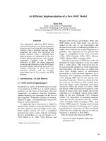
84.2% reliability rate was obtained with recording 616 hours as cycle time for the entire supply chain
system. The delay was minimized and reached to 37 hours. The performance and reliability rate of the
system at 84.2% (Fig. 3).

Distribution for each Reliability Target
0.07
0.06

Curve for Reliability of
73.8%

0.05

PDF

0.04
0.03
Curve for Reliability of
84.2%

0.02
0.01
0
0

50

100

150

Cycle Time

Fig.3. Distribution of mean total cycle time
By running the model, the reliability rate of each entity was improved which achieved value beyond
the target and recorded 84.2%. Also, the cost of improving the supply chain system to reach a reliability
rate of 84.2% was $ 26,550. Table 6 and Table 7 show the initial and improved values.
Table 6
The initial and optimal reliability rates each entity
Entity
Supplier j=1
Route j=2
Factory j=3
Route j=4
DC j=5
Route j=6
Customer j=7

Initial Reliability Rate
0.958
0.933
0.929
0.921
0.893
0.925
0.939

Obtained Reliability Rate

0.986
0.974
0.976
0.969
0.970
0.972
0.980

Table 7
The overall initial and optimal reliability rates.
Initial Reliability
60.9%

Reliability Target
80%

Obtained Reliability Rate
84.2%

Total Cost
$26,550

Since the objective of this case study is to lead the system to 90 reliability rate zone as well as obtaining
minimum possible cost, the reliability target was changed to 90%. The following values identify the
optimal mean and standard deviation with their reduction cost intervals.


392

Mean Time Reduction

StandardDeviation Reduction

1200

80 95

83

2,160 84

81

1100

50 72

62

1,60063

60

1000

80 88

77

1,96079

76

1100

50 90

80

1,60081

78

1400

90 101

3,11083

80

1100

50 80

70

1,60071

68

1200

80 77

64

2,240 65

62

82

1300

80 21

5

2,58006

03

1000

70 17

4

1,91005

03

1200

80 18

5

2,24006

03

1100

80 22

5

2,46007

04

1400

110 24

3,38006

03

1300

80 20

2,58005

02

1500

100 14

2,70002

00

6
4
2

Also, the obtained cycle time was 571 hours with recording only 20 hours as delay time for the overall
supply chain system. The performance and reliability rate of the system at 90.59% is represented by
the line legend in Fig. 4.

PDF

Distribution for Each Target
0.1
0.09

0.08
0.07
0.06
0.05
0.04
0.03
0.02
0.01
0

Curve for Reliability of
73.8%
Curve for Reliability of
84.2%
Curve for Reliability of
90.59%
0

20

40

60

80

100

120

140

Cycle Time

Fig.4. Distribution of mean total cycle time
After running the model, the reliability rate of each entity was improved to achieve the target of 90.59%
as an overall rate. Also, the model ensured possible minimum cost of improving the entire supply chain
which was only $ 32,120 to achieve the required target. Table 8 and Table 9 show the initial and
improved reliability rates.
Table 8
Initial and optimal reliability rates each entity.
Entity
Supplier j=1
Route j=2
Factory j=3
Route j=4
Distribution Center j=5
Route j=6
Customer j=7

Initial Reliability Rate
0.958
0.933
0.929
0.921
0.893
0.925
0.939

Obtained Reliability Rate

0.990
0.986
0.984
0.984
0.982
0.986
0.991


393

Y.H. Daehy et al. /Uncertain Supply Chain Management 7 (2019)
 

Table 9
The overall initial and optimal reliability rates.
Initial Reliability
Reliability Target
Obtained Reliability Rate
60.9%
90%
90.59%

Total Cost
$32,120

It is clear, that there is a negative correlation between cost and time in the model. In order to improve
processing activities, which results in reducing cycle time, additional money has to be invested. Also,
to reduce the uncertainty factors money has to be invested as well. Fig. 5 shows the different total cost
at different reliability targets. By applying the MATLAB model, the cycle time of each process in

supply chain system is acquired as well as the overall cycle time.

Fig. 5. Cost of optimizing reliability rate of supply chain system
It is obvious that there are varied differences in cost between the different reliability targets achieved
after applying the model. The system at first target spent $ 19,280 as reduction cost while the optimized
system at 90.59% reliability rate recorded about $ 32,120 as cost for time reduction. The results of the
case study are shown in Table 10. Table 10 shows the initial mean time at each entity, as well as the
optimal mean time. For example, the supplier’s initial mean time reached to 95, whereas the optimal
mean time for the same entity recorded minimum value, which was steady at 83 hours.
Table 10
Initial and optimal mean time.
Process
S
R1-2
F
R2-3
DC
R3-4
V

Initial Mean time
95
72
89
90
101
80
77

Optimal Mean Time

83
62
77
80
82
70
66

In addition, each achieved reliability target has also identified the cycle time that has to be obtained in
order to achieve the reliability target. Table 11 and Fig. 6 shows the improvement in cycle time as well
as the reliability rate.
Table 11
The optimal cycle time with obtained reliability rate
Optimal Cycle Time hour
Reliability Rate

840
60.9%

696
73.8%

616
84.2%

571
90.59%


394

System Reliability Improvement
100
90
80
70
60
50
40
30
20
10
0
59%

73%

84.20%

90.50%

Fig. 6. illustrates System Reliability Improvement
From Table 11, while the initial cycle time for delivering one batch was 840 hours, with optimization
the cycle time has been reduced to 571 hours. The delay recorded is only 20 hours per batch. Also, the
reliability rate increased to reach the rate of 90.59%. Hence, all constraints and requirements, such as
the overall supply chain system reliability rate and the optimal total cost, were satisfied.
6. Conclusion and Future Study
There is always a need to address the reliability concept in supply chain system as more companies,
departments, organizations, and other divisions are being involved in the supply chain’s structure. Also,
from a business perspective, minimizing costs is a significant matter that has to be addressed to have

reliable and robust supply chain system. This research has concentrated on evaluating reliability rates
at each entity through the supply chain system. Also, this work explains how the supply chain system
optimization model could be applied to obtain minimum possible total cost while fulfilling the
reliability requirements. Moreover, applying different scenarios of reliability targets makes the model
more applicable to utilize for different business sectors. The effects of uncertainty driven by production
and transportation on overall reliability were examined in the paper as well. Results and analysis of this
study have accentuated that the presented mathematical model can be applied to rebuild the supply
chain system where the system can be improved to reach a desired reliability target, which can be used
as a guide to design supply chain systems that reduces costs. In conclusion, the optimization approach
that has been presented in this study is to provide an appropriate method that helps to satisfy the
reliability requirements at the minimum possible cost. Also, the mathematical model has the flexibility
and the potential to be implemented for any supply chain system regardless to the complexity or the
type of the system. As a future study, this study will spend more investigation in how reliability
performance affects the total cost of managing internal and external subsystems in the supply chain, as
well as for the overall supply chain system. Also, it will continue to consider multi-products factor and
multi-levels (complex) supply chain systems.


Y.H. Daehy et al. /Uncertain Supply Chain Management 7 (2019)

395

 

References
Almaktoom, A. T., Krishnan, K. K., Wang, P., & Alsobhi, S. (2014). Assurance of system service level
robustness in complex supply chain networks. The International Journal of Advanced
Manufacturing Technology,74(1-4), 445-460.
Almaktoom, A. T. (2017). Stochastic reliability measurement and design optimization of an inventory
management

system. Complexity, 2017.
Article
ID
1460163,
9
pages,
2017.
doi:10.1155/2017/1460163.
Bayat, Y., Pourmortazavi, S. M., Ahadi, H., & Iravani, H. (2013). Taguchi robust design to optimize
supercritical carbon dioxide anti-solvent process for preparation of 2, 4, 6, 8, 10, 12-hexanitro-2, 4,
6, 8, 10, 12-hexaazaisowurtzitane nanoparticles. Chemical Engineering Journal, 230, 432–438.
Chen, W., Wiecek, M. M., & Zhang, J. (1999). Quality utility—a compromise programming approach
to robust design. Journal of Mechanical Design, 121(2), 179-187.
Christopher, M., Mena, C., Khan, O., & Yurt, O. (2011). Approaches to managing global sourcing risk.
Supply Chain Management: An International Journal, 16(2), 67–81.
Cooper, M. C., Lambert, D. M., & Pagh, J. D. (1997). Supply chain management. More than a new
name for logistics. The International Journal of Logistics Management, 8(1), 1-13.
Deb, K. (2001). Multi-objective optimization using evolutionary algorithms (Vol. 16). John Wiley &
Sons.
Eggert, R. J., & Mayne, R. W. (1993). Probabilistic optimal design using successive surrogate
probability density functions. Journal of Mechanical Design, 115(3), 385-391.
Eruguz, A. S., Jemai, Z., Sahin, E., & Dallery, Y. (2013, April). Cycle-service-level in guaranteedservice supply chains. In Modeling, simulation and applied optimization (ICMSAO), 2013 5th
International Conference on (pp. 1-6). IEEE.
Garvin, D. A. (1984). What Does “Product Quality” Really Mean?. Sloan Management Review, 25-42.
Goh, M., & Pinaikul, P. (1998). Logistics management practices and development in Thailand.
Logistics Information Management, 11(6), 359-369.
Gu, D. W., Petkov, P. H., & Konstantinov, M. M. (2013). Robust control of a hard disk drive. In Robust
Control Design with MATLAB® (pp. 249-290). Springer, London.
Gunasekaran, A., Patel, C., & McGaughey, R. E. (2004). A framework for supply chain performance
measurement. International journal of production economics, 87(3), 333-347.

Gunasekaran, A., Patel, C., & Tirtiroglu, E. (2001). Performance measures and metrics in a supply
chain environment. International journal of operations & production Management, 21(1/2), 71-87.
Hwang, K. H., Lee, K. W., & Park, G. J. (2001). Robust optimization of an automobile rearview mirror
for vibration reduction. Structural and Multidisciplinary Optimization, 21(4), 300-308.
So, K. C. (2000). Price and time competition for service delivery. Manufacturing & Service Operations
Management, 2(4), 392-409.
Kleijnen, J. P., & Smits, M. T. (2003). Performance metrics in supply chain management. Journal of
the Operational Research Society, 54(5), 507-514.
Konak, A., Coit, D. W., & Smith, A. E. (2006). Multi-objective optimization using genetic algorithms:
A tutorial. Reliability Engineering & System Safety, 91(9), 992–1007.
Laosirihongthong, T., & Dangayach, G. S. (2005). A comparative study of implementation of
manufacturing strategies in Thai and Indian automotive manufacturing companies. Journal of
Manufacturing Systems, 24(2), 131-143.
Li, S., Okoroafo, S. & Gammoh, B. (2014). The role of sustainability orientation in outsourcing:
Antecedents, practices, and outcomes. Journal of Management and Sustainability, 4(3), 27-36.
Mentzer, J. T., DeWitt, W., Keebler, J. S., Min, S., Nix, N. W., Smith, C. D., & Zacharia, Z. G. (2001).
Defining supply chain management. Journal of Business logistics, 22(2), 1-25.
Mentzer, J. T., Myers, M. B., & Cheung, M. S. (2004). Global market segmentation for logistics
services. Industrial marketing management, 33(1), 15-20.


396

Murata, T., Ishibuchi, H., & Tanaka, H. (1996). Multi-objective genetic algorithm and its applications
to flow shop scheduling. Computers & Industrial Engineering, 30(4), 957–968.
Nixon, P., Harrington, M., & Parker, D. (2012). Leadership performance is significant to project
success or failure: a critical analysis. International Journal of Productivity and Performance
Management, 61(2), 204-216.
Peng, W., Huang, H. Z., Zhang, X., Liu, Y., & Li, Y. (2009). Reliability based optimal preventive
maintenance policy of series-parallel systems. Eksploatacja i Niezawodność, 4-7.

Phadke, M. S. (1995). Quality Engineering Using Robust Design: Prentice Hall PTR, Upper Saddle
River, NJ.
Rambau, J., & Schade, K. (2010). The stochastic guaranteed service model with recourse for multiechelon warehouse management. Electronic Notes in Discrete Mathematics, 36, 783-790. Chicago.
Saad, M., Jones, M., & James, P. (2002). A review of the progress towards the adoption of supply chain
management (SCM) relationships in construction. European Journal of Purchasing & Supply
Management, 8(3), 173-183.
Tu, J., Choi, K. K., & Park, Y. H. (1999). A new study on reliability-based design optimization. Journal
of mechanical design, 121(4), 557-564.
Waller, D. L. (2003). Operations management: a supply chain approach. Cengage Learning Business
Press.
Yadav, O. P., Bhamare, S. S., & Rathore, A. (2010). Reliability‐based robust design optimization: A
multi‐objective framework using hybrid quality loss function. Quality and Reliability Engineering
International, 26(1), 27–41.
Yildirim, M. B., & Mouzon, G. (2012). Single-machine sustainable production planning to minimize
total energy consumption and total completion time using a multiple objective genetic algorithm.
IEEE Transactions on Engineering Management, 59(4), 585–597.
Youn, B.D., & Wang, P. (2009). Complementary Interaction Method (CIM) for System Reliability
Assessment. Journal of Mechanical Design, 131(4), 041004(15).
Zeithaml, V. A., & Parasuraman, A. (2004). Service quality.
Appendix A
Costs of Reduction for Each Entity in The Supply Chain System
Amount of Time Intervals Reduction and Associated Costs of Reduction
700
50 95
Mean Time
Supplier (S)

Reduction

800

for

Mean Time Reduction

60 95

93

95

93

90

93

90

1000

70 95

87

90

87

1100

80 95

84

87

84

1200

80 95

81

84

81

1300

80 95

78

81

78

80 95

75

78

75

1400
Standard Deviation Reduction for
Supplier (S)

Standard Deviation Reduction

800

40 21

18

21

18

900

50 21

15

18

15

1000

70 21

12

15

12

1100

80 21

9

12

09

1200

80 21

6

09

06

1300

80 21

3

06

03

1400

80 21

2

03

02


397

Y.H. Daehy et al. /Uncertain Supply Chain Management 7 (2019)
 

Mean Time Reduction for Route

(R)

700

Mean Time Reduction

1000

40 72

63

66

63

1100

50 72

60

63

60

1200

60 72

57

StandardDeviation Reduction

Mean Time Reduction

54

80 72

51

54

51

600

30 17

14

17

14

700

40 17

11

14

11

800

50 17

08

11

08

900

60 17

5

08

05

1000

70 17

3

05

03

1100

80 17

0

03

00
85

800

70 88

82

85

82

1000

70 88

79

82

79

1000

80 88

76

79

76

1200

80 88

73

76

73

1300

90 88

70

73

70

67

70

67

80 88
800

40 18

15

18

15

900

50 18

12

15

12

1000

70 18

09

12

09

1100

80 18

6

09

06

1200

80 18

3

06

03

1300

80 18

0

03

20 90

87

90

00
87
84

800

30 90

84

87

1000

40 90

81

84

81

1100

50 90

78

81

78

1200

78

75

1300

70 90

72

75

72

1400

80 90

69

72

69

Standard Deviation Reduction for
Route (R)

StandardDeviation Reduction

Mean Time Reduction

57

88

700

for

57

54

85

StandardDeviation Reduction

Mean Time Reduction
Distribution (DC)

60

70 72

50 88

1400

Mean Time Reduction

66

800

Standard Deviation Reduction for
Factory (F)

Mean Time Reduction for Route

(R)

69

69

1400

for

72

66

Standard Deviation Reduction for
Route (R)

Reduction

69

30 72

1300

Mean Time
Factory (F)

20 72

800

60 90

75

600

30 22

19

22

19

700

40 22

16

19

16

800

50 22

13

16

13

900

60 22

10

13

10

1000

70 22

7

10

07

1100

80 22

4

07

04

800

50 101

98

101

98

800

70 101

95

98

95
92

1000

70 101

92

95

1000

80 101

89

92

89

1200

80 101

86

89

86

1300

90 101

83

86

83

1400

90 101

80

83

80


398
Standard Deviation Reduction for
Distribution (DC)

StandardDeviation Reduction

Mean Time Reduction for Route
(R)

Mean Time Reduction

for

Mean Time Reduction

21

24

21

900

50 24

18

21

18

1000

70 24

15

18

15

1100

80 24

12

15

12

1200

90 24

09

12

09

1300

100 24

06

09

06

1400

110 24

03

06

03

20 80

77

80

77

800

30 80

74

77

74

1000

40 80

71

74

71

1100

50 80

68

71

68

1200

60 80

65

68

65

1300

70 80

59

65

62

1400

80 80

56

62

59

StandardDeviation Reduction

Reduction

40 24

700

Standard Deviation Reduction for
Route (R)

Mean Time
Customer (V)

800

700

30 20

17

20

17

800

40 20

14

17

14

900

50 20

11

14

11

1000

60 20

08

11

08

1100

70 20

5

08

05

1300

80 20

2

05

02

2000

90 20

0

02

00

800

50 77

74

77

74

800

70 77

71

74

71

1000

70 77

68

71

68

1000

80 77

65

68

65

1200

80 77

62

65

62

1300

90 77

59

62

59

1400

90 77

56

59

56

Standard Deviation Reduction for
Customer (V)
StandardDeviation Reduction

1000

40 14

11

14

11

1100

50 14

1200

70 14

08

11

08

5

08

05

1300

80 14

2

05

02

1500

100 14

02

00

0

© 2019 by the authors; licensee Growing Science, Canada. This is an open access
article distributed under the terms and conditions of the Creative Commons Attribution
(CC-BY) license ( />