Interpreting comprehensive two-dimensional gas chromatography using peak topography maps with application to petroleum forensics

Ghasemi Damavandi et al. Chemistry Central Journal (2016) 10:75
DOI 10.1186/s13065-016-0211-y

RESEARCH ARTICLE

Open Access

Interpreting comprehensive
two‑dimensional gas chromatography using
peak topography maps with application
to petroleum forensics
Hamidreza Ghasemi Damavandi1†, Ananya Sen Gupta1*†, Robert K. Nelson2 and Christopher M. Reddy2

Abstract 
Background:  Comprehensive two-dimensional gas chromatography (GC × GC) provides high-resolution separations across hundreds of compounds in a complex mixture, thus unlocking unprecedented information for intricate
quantitative interpretation. We exploit this compound diversity across the (GC × GC) topography to provide quantitative compound-cognizant interpretation beyond target compound analysis with petroleum forensics as a practical application. We focus on the (GC × GC) topography of biomarker hydrocarbons, hopanes and steranes, as they
are generally recalcitrant to weathering. We introduce peak topography maps (PTM) and topography partitioning
techniques that consider a notably broader and more diverse range of target and non-target biomarker compounds
compared to traditional approaches that consider approximately 20 biomarker ratios. Specifically, we consider a range
of 33–154 target and non-target biomarkers with highest-to-lowest peak ratio within an injection ranging from 4.86
to 19.6 (precise numbers depend on biomarker diversity of individual injections). We also provide a robust quantitative measure for directly determining “match” between samples, without necessitating training data sets.
Results:  We validate our methods across 34 (GC × GC) injections from a diverse portfolio of petroleum sources, and
provide quantitative comparison of performance against established statistical methods such as principal components analysis (PCA). Our data set includes a wide range of samples collected following the 2010 Deepwater Horizon
disaster that released approximately 160 million gallons of crude oil from the Macondo well (MW). Samples that
were clearly collected following this disaster exhibit statistically significant match (99.23 ± 1.66) % using PTM-based
interpretation against other closely related sources. PTM-based interpretation also provides higher differentiation
between closely correlated but distinct sources than obtained using PCA-based statistical comparisons. In addition to
results based on this experimental field data, we also provide extentive perturbation analysis of the PTM method over
numerical simulations that introduce random variability of peak locations over the (GC × GC) biomarker ROI image
of the MW pre-spill sample (sample #1in Additional file 4: Table S1). We compare the robustness of the cross-PTM
score against peak location variability in both dimensions and compare the results against PCA analysis over the same

set of simulated images. Detailed description of the simulation experiment and discussion of results are provided in
Additional file 1: Section S8.

*Correspondence: ananya‑
†
Hamidreza Ghasemi Damavandi and Ananya Sen Gupta contributed
equally to this work
1
Department of Electrical Engineering, University of Iowa, 103 S Capitol
Street, Iowa City, IA 52242, USA
Full list of author information is available at the end of the article
© The Author(s) 2016. This article is distributed under the terms of the Creative Commons Attribution 4.0 International License
( which permits unrestricted use, distribution, and reproduction in any medium,
provided you give appropriate credit to the original author(s) and the source, provide a link to the Creative Commons license,
and indicate if changes were made. The Creative Commons Public Domain Dedication waiver ( />publicdomain/zero/1.0/) applies to the data made available in this article, unless otherwise stated.


Ghasemi Damavandi et al. Chemistry Central Journal (2016) 10:75

Page 2 of 14

Conclusions:  We provide a peak-cognizant informational framework for quantitative interpretation of (GC × GC)
topography. Proposed topographic analysis enables (GC × GC) forensic interpretation across target petroleum biomarkers, while including the nuances of lesser-known non-target biomarkers clustered around the target peaks. This
allows potential discovery of hitherto unknown connections between target and non-target biomarkers.
Keywords:  GC × GC, Chromatography, Principal component analysis, Multivariate statistics, Quantitative
interpretation, Oil-spill forensics

Background
Comprehensive two-dimensional gas chromatography
(GC × GC) provides high-resolution separation across

hundreds, sometimes thousands, of crude oil hydrocarbons, thus unlocking unprecedented information for
intricate quantitative interpretation. The broad objective
of this work is to exploit this rich compound diversity
and provide compound-cognizant quantitative interpretation of (GC × GC) peak topography that bridges the
gap between target-driven analysis and statistical methods. We propose peak topography maps that extend individual (GC × GC) peak analysis beyond the well-known
target peaks that dominate the (GC × GC) image, and
present techniques for interpreting (GC × GC) topography that provide nuanced quantitative peak-based comparisons between (GC × GC) images. While we present
our results in the context of petroleum forensics as a
practical application of interest, the scope of our work
applies generally to quantitative (GC × GC) interpretation and as such, goes beyond the stated application.
A key distinction of our technique against multi-variate statistical methods [1] is compound-cognizant interpretation that preserves the identity of individual target
peaks while extending the scale of peak-level interpretation to all peaks, target and non-target, within the
(GC × GC) topography. This allows nuanced (GC × GC)
distinction between closely related yet different complex
mixtures, e.g. crude oil from neighboring oil sources,
which share the regional fingerprint, and therefore, difficult to differentiate robustly using purely statistical
methods.
Current state‑of‑the art in chromatographic interpretation:
challenges and opportunities

Many separation technologies routinely filter out nontarget analytes, thus eliminating possibility of understanding their connection to dominant target analytes
in an environmental sample. More comprehensive data
sets recording the joint contributions of target and nontarget analytes may be enabled through comprehensive two-dimensional gas chromatography (GC × GC) ,
liquid chromatography (LC × LC), mass spectrometry
(MS) and combinations thereof. However, despite the
informational richness of these comprehensive data sets,

non-target analytes are traditionally ignored in sample
analysis in preference to peak ratio comparisons between
the target chemicals. Although non-target chemicals are

empirically considered in the chemometric literature,
their role is typically limited to the major statistical loadings in multi-variate distributions [2–4]. Thus, current
state-of-the-art in environmental forensics and analytical
chemistry are broadly divided into two complementary
approaches:
••  Target-based analysis [3–14]: Focuses on the target
chemicals (well-known hopanes, steranes, diasteranes in petrochemicals) that dominate the analytical
landscape as the major peaks in a chromatogram or
a GC–MS image. This includes statistical methods
employed towards target-based analysis [12, 15].
••  Target-agnostic analysis [16–22]: Statistical patternrecognition techniques that analyze comprehensive
separation data sets using different forms of multivariate analysis.
Additional file  2: Table S7 (in Section S7) provides a
point-by-point comparison between the two approaches
in the context of environmental forensics.
Petroleum forensics using GC × GC separation of crude oil
samples

Reliable fingerprinting of petroleum and its weathered
products has been an important field of study in the
last four decades [2–10, 23–31]. Forensic analysis techniques fingerprinting crude oil samples in the ocean typically interpret the GC × GC peak profiles of biomarker
hydrocarbons (hopanes and steranes), as they are generally recalcitrant against environmental weathering
[4, 7, 11, 25–31]. Figure  1 shows the GC × GC hopanesterane biomarker topography as the region of interest
(ROI) within the full chromatogram of a pre-spill crude
oil sample taken from the Macondo well  (MW), source
of the Deepwater Horizon disaster. The ROI biomarker
region spans over a hundred compounds across a relative scale of 1−14.53 between the lowest and highest
summits (peaks occupying lowest 5  % of the GC × GC
peak magnitude profile were rejected as baseline noise).
Traditional analysis employs approximately forty target

Ghasemi Damavandi et al. Chemistry Central Journal (2016) 10:75

Fig. 1  a The three-dimensional view of detailed topography of
biomarker region (hopanes and steranes) within GC × GC image of
crude oil pre-spill sample from MW, site of Deepwater Horizon spill
disaster, Gulf of Mexico, 2010. b Biomarker region (hopanes and
steranes) of (a) marked as the region of interest (ROI), shown as red
box within full chromatogram.Target biomarkers within this ROI are
labeled and itemized in Table S2. Total number of detected biomarker
peaks (target and non-target) = 111, after removing peaks occupying
lowest 5 % of the GC × GC peak magnitude profile as baseline noise.
Range of considered peak summits (highest:lowest) = 14.53:1 (Aeppli
et al. [25] Nelson et al. [36])

biomarker compounds [refer to labeled compounds in
Additional file  3: Table S2 (in Section S2)], which occur
as major peaks dominating the GC × GC ROI biomarker
topography, and about twenty well-known peak ratios
[25] based on these target compounds.
Background motivation: peak‑cognizant interpretation
beyond target biomarkers

Target biomarkers are generally abundant within a sample, robust to chromatographic variability, and therefore, provide a well-established basis to compare two
oil samples [3, 4, 6, 7, 25]. However, the interpretation
power of target analysis can be magnified significantly
if we harness the full informational potential GC × GC :
combining the well-known characteristics of target biomarkers (major peaks) with the lesser known nuances
of non-target biomarkers (minor peaks), which occupy

the breadth of the intricate GC × GC topography. More
recently, chemometric interpretations of GC × GC data
sets have been proposed that adopt a multi-variate statistical approach to forensic interpretation [15–18, 32–34].

Page 3 of 14

While these statistical approaches exploit the data variance of the GC × GC topography beyond the target
peaks, they are typically agnostic of the target biomarkers and the dominant role they play in forensic interpretation [3, 4, 6–10, 25]. We harness the rich compound
diversity across the GC × GC biomarker (hopanes and
steranes) topography to provide potentially transformative compound-cognizant interpretation beyond target
compound analysis.
Our objective is to extend the scope of target-centric standards [8–10] to include non-target biomarkers within a compound-cognizant framework, and thus
bridge the gap between target-based forensics (e.g. [3,
4, 6, 7, 25] and references therein) and existing targetagnostic statistical approaches [15–17, 32–34]. We
achieve source-specific and regional fingerprints by
mapping connections between target and non-target
biomarkers within the GC × GC topography. While the
established target peaks dominate forensic interpretation, and can be individually identified in the topography
map proposed, the unutilized contribution of the minor
(non-target) peaks (e.g. the 73 unlabeled non-target
peaks in Fig. 1) are also employed to distinguish closely
related samples. Furthermore, we propose partitioning
techniques that enable discovery of peak clusters connecting known targets to unknown non-target biomarkers, and thus derive common regional characteristics of
petroleum-rich areas.
Key innovation and contributions

Our motivation in this work is to achieve robust forensic
distinction between closely related oil sources by utilizing rich peak information diversity in GC  ×  GC chromatography. We validate our peak topographic methods
across a set of 34 GC × GC injections from a diverse
portfolio of petroleum sources, including a wide range of

samples collected from the MW, the source of the Deepwater Horizon disaster in the Gulf of Mexico, April 2010.
The MW samples exhibit statistically significant match
(99.23 ± 1.66%) against other closely related sources
(Table  1). We introduce peak mapping and partitioning
techniques that combine source-specific and regional
characteristics manifested through the GC × GC topography of neighboring oil sources. We also provide a
robust quantitative measure for directly determining
“match” between samples, without necessitating training data sets. This is a key distinction against supervised
learning techniques [19–22] that necessitate strong
ground truths derived from large training databases that
may be difficult to avail in the event of localizing a natural seep or surveying connectivity between newly discovered oil prospects. Our contribution is summarized in
three novel concepts introduced in this work:


Ghasemi Damavandi et al. Chemistry Central Journal (2016) 10:75

Page 4 of 14

Table 1  Percentage match (Mean ± standard deviation) between different Gulf of Mexico sources against MW injections
for PTM with the optimal choice of peak ratio threshold (τ = 1.65) and for PCA with two principal components
Method

MW (%) vs. MW (%)

Eugene Island (%) vs. MW (%)

PTM

99.23 ± 1.66

85.83 ± 3.70

59.28 ± 13.34

52.55 ± 1.94

PCA

99.76 ± 0.26

91.98 ± 0.14

91.71 ± 0.24

98.01 ± 0.51

••  Peak topography map (PTM), a feature representation that collectively captures GC × GC topography
derived from the GC × GC chromatogram,
••  Topography partitions, a threshold-based partitioning technique for discovering source-specific and
regional characteristics, and
••  Cross-PTM analysis, mathematical technique for
directly determining “match” between two GC × GC
separations without needing training data sets.
A natural outcome of PTM-based analysis is the discovery of topographic clusters (closely eluting groups
of target and non-target biomarkers), which are key
to understanding the regional and source-specific
fingerprint.

Experimental
Additional file 4: Table S1 (in Section S1) lists the thirtyfour injections along with the corresponding details on

sample identity and geographic origin. The injections
may be classified into three groups:
••  Fourteen injections clearly originating from the MW,
source of the Deepwater Horizon disaster;
••  Three injections from non-Macondo well oil originating from three different sources in the Gulf of
Mexico; and,
••  Seventeen injections from diverse oil sources outside
the Gulf of Mexico region.
In particular, injections 1 and 2 correspond to independent injections of a pre-spill sample taken directly from
the MW during normal operations before the disaster;
injection 3 corresponds to a surface slick sample from
the MW collected after the spill; injection 4 is a postspill sample collected directly from the broken riser pipe
on June 21, 2010 [28, 35]; injections 5 through 14 correspond to ten separate oil samples that were obviously
from the MW spill collected from grass blades along the
Louisiana Gulf of Mexico coast; injections 15 and 16 are
from two other crude oil sources from northern Gulf of
Mexico and were collected before the Deepwater Horizon disaster, and injection 17 is collected from a natural

Southern Louisiana Crude (SLC)
(%) vs. (MW) (%)

Natural seep (%) vs.
(MW) (%)

oil seep in the Gulf of Mexico in 2006. The remaining
injections correspond to distant sources unrelated to the
Gulf of Mexico. For example, injections 18, 19 and 20
are independent consecutive injections of the National
Institute of Standards and Technology (NIST) Standard
Reference Material 1582 (its characteristics suggest it

is derived from Monterey Shale and likely a California
crude similar to injection 21).
GC × GC ‑flame ionization detector (FID) analysis

The samples were analyzed on a GC × GC -FID system
equipped with a Leco dual stage cryogenic modulator
installed in an Agilent 7890A gas chromatograph configured with a 7683 series split/splitless auto-injector, two
capillary columns, and a flame ionization detector. Samples were injected in splitless mode, and the split vent
was opened at 1.0 minutes. The inlet temperature was
300  °C. The first-dimension column and the dual stage
cryogenic modulator reside in the main oven of the Agilent 7890A gas chromatograph. The second-dimension
column is housed in a separate oven installed within the
main GC oven. With this configuration, the temperature
profiles of the first-dimension column, dual stage thermal
modulator, and the second-dimension column can be
independently programmed. The first-dimension column
was a Restek Rtx−1, (30 m, 0.25 mm I.D., 0.25 µm film
thickness) that was programmed to remain isothermal at
45 °C for 10 min and then ramped from 45 to 315 °C at
1.2  °C min−1. Compounds eluting from the first dimension column were cryogenically trapped, concentrated,
and re-injected (modulated) onto the second dimension
column. The modulator cold jet gas was dry nitrogen,
chilled with liquid nitrogen. The thermal modulator hot
jet air was heated to 45 °C above the temperature of the
main GC oven (thermal modulator temperature offset =
45  °C). The hot jet was pulsed for 1.0  s every 12  s with
a 5.0 s cooling period between stages. Second-dimension
separations were performed on a SGE BPX50 (1 m, 0.10
mm I.D., 0.1 µm film thickness) that remained at 75  °C
for 10 min and then ramped from 75 to 345 °C at 1.2 °C

min−1. The carrier gas was hydrogen at a constant flow
rate of 1.1 mL min−1. The FID signal was sampled at 100
data points s−1.


Ghasemi Damavandi et al. Chemistry Central Journal (2016) 10:75

Methods

We introduce the PTM representation of GC × GC data
as an informational method that characterizes the peak
information across the GC × GC biomarker topography as a connected graph. Wherever applicable in this
work, peak refers to a single second-dimension peak,
and GC × GC ROI refers to the biomarker sub-region
(hopanes and steranes) of a two-dimensional gas chromatogram. Figure 1 illustrates this biomarker ROI within
the full GC× GC chromatogram of the MW pre-spill
sample listed as sample #1 in Table S1. We focus on the
hopane-sterane biomarker topography as the region of
interest (ROI) as these compounds are well-known for
their recalcitrance to environmental degradation [25, 36].
Peak topography map (PTM) representation

PTM is a scalable node-based representation computed
over a pre-selected GC × GC ROI representing the biomarker compounds. The PTM representation is scalable
because: (i) PTM computation can be scoped to a smaller
sub-region within the chosen GC × GC ROI, and (ii)
PTMs computed across disjoint GC × GC ROIs can be
combined to construct the PTM across the union of these
regions, e.g. PTMs for the hopanes and steranes can be
computed separated and then combined to give the PTM

over both hopanes and steranes. Each PTM consists of
a two-dimensional node structure that preserved peak
characteristics, e.g. peak height, peak location and order
of elution.
Mathematically, each peak collapses into a single PTM
node that stores two attributes: (i) the magnitude at the
peak summit, and (ii) peak location. We represent information at a PTM node (denoted as η) with the value
assignment η = {p, m, n}, where p denotes the peak summit value, and m and n respectively denote the first and
second dimension retention time indices for the particular peak in the GC × GC image.
The nodes are stored as an ordered two-dimensional
matrix, with the first dimension coinciding with the first
dimension retention time indices and the second dimension storing the PTM nodes in the consecutive order of
elution of peaks along the second dimension. Thus the
[q,  m]-th element of the PTM matrix with node value
η = {p, m, n} stores the qth compound with peak height
p, eluting along the second dimension with peak location [n,  m] in the GC × GC image. The number of columns N of the PTM matrix represents the total number
of first dimension modulations for the GC × GC ROI.
The number of rows Q represents the maximum number
of peaks eluting along the second dimension within the
GC × GC ROI. The maximum number of peaks is computed across all second dimension indices within the
GC × GC ROI. A PTM matrix column with fewer peaks

Page 5 of 14

than Q stores the PTM nodes in ascending order of peak
locations, and populates the remaining entries with zeros
to denote absence of a peak in those PTM nodes. We
will henceforth refer to these entries in the PTM matrix
that do not have a peak as “blank nodes”. To compute the
PTM of a GC × GC ROI we normalize the PTM against

the maximum value of the peaks. This normalization nullifies the effect of variable signal strengths between different injections by measuring all peak heights relative
to the maximum signal strength within each GC × GC
ROI. We locate all peaks within this ROI by employing
a gradient-based maxima search (ref. Additional file  5:
Section S4). Peaks that fall below 5 % of the maximum
peak height within the GC × GC ROI are rejected as
baseline noise. Mathematically, suppose the nth column of a GC × GC image has κn number of peaks. The
amplitudes and the locations of the peaks in this column can be stored in Peakn = {p1,n , p2,n , . . . , pκn ,n } and
Locn = {m1,n , m2,n , . . . , mκn ,n }. We construct the (l, n)th
element of its PTM representation matrix as:

PTM[l, n] =

pl,n + j × ml,n if 1 ≤ l ≤ κn
0
if l > κn

(1)

In other words, if l corresponds to a peak location along
the nth column of the GC × GC image, then the (l, n)th
node of the PTM is a complex number with its real part
as the amplitude of the peak and the imaginary part as its
location. In case l does not correspond to a peak, (l, n)
th node will be zero. Therefore, the problem of comparing two GC × GC image, like Itest and Iref will turn into
the problem of comparing the nodes at the same location
in their PTM representation matrices. Figure 2 provides a
visual representation of PTM computation for the crude
oil MW pre-spill sample in Fig. 1 collected from the MW,
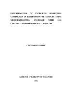
Gulf of Mexico (injection 1 in Table S1). Figure 3 shows

the full chromatogram, two and three-dimensional plots
of the biomarker ROI and the PTM matrix corresponding
to a sample from Eugene Island, another Gulf of Mexico
source. The 38 target PTM nodes labeled for identification with the target compounds in the ROI biomarker
region (detailed in Table S2) are highlighted in the constructed PTM matrix. We note that the PTM matrices for
the MW pre-spill sample (Fig. 2) and the Eugene Island
sample (refer Fig. 3) are visually easier to distinguish than
the original biomarker ROI image.
Target compounds align according to their order of
elution along the second dimension rather than absolute coordinates by design, thus rendering their location with respect to relative order of elution instead of
specific retention times. Additional file  6: Algorithm  1
(in Section S3.1) and Additional file  7: Section S3.2
detail computational methods for ensuring PTM nodes
compared across injections store the same compound


Ghasemi Damavandi et al. Chemistry Central Journal (2016) 10:75

Page 6 of 14

Fig. 2  Step-by-step PTM construction Target biomarkers are labeled and itemized in Table S2. Total number of detected biomarker peaks (target
and non-target) = 111, after removing peaks occupying lowest 5 % of the GC × GC peak magnitude profile as baseline noise. Range of considered
peak summits (highest:lowest) = 14.53:1

within a pre-selected variability threshold. Local indexing of peak nodes with respect to relative order of elution instead of specific retention times makes the PTM
interpretation robust to chromatographic variability
within bounds { 1 , 2 } (refer Additional file 6: Section
S3, Algorithm 1) of expected variability selected by the
user. Additional file  1: Section S8 and related discussion in the "Results" section also provides in-depth perturbation analysis of PTM interpretation against peak
location variability. In summary, we observed that the

PTM approach is relatively immune to variability even
when introduced variability is greater than the bounds
{ 1 , 2 } of expected variability selected by the user.
Topography partitioning: direct GC × GC comparisons based
on aligned PTMs

We introduce topography partitioning as a visual quantitative informational method to facilitate direct comparison between two GC × GC ROIs. Topography partitions

provide intricate cross-comparison between oil samples
highlighting nuances of their biomarker topographies.
Topography partitions also form the basis for the crossPTM score: a novel threshold-driven quantitative metric
that provides a single numerical score for determining
whether the two samples are a match. The key idea is
to partition the GC × GC biomarker topography of a
test sample based on which peaks, target and non-target, match against that of a reference sample using their
respective PTM representations.
Mathematical computation of topography partitions  The
peak-level match is determined using a peak ratio metric
(ref. Equation S3.1 in Algorithm 1). This peak ratio metric is
calculated at the granularity of individual PTM nodes and
assessed against a pre-selected threshold to decide a match
between the test and reference samples for a given compound. These individual match assessments are then conducted across peak profiles spanning the GC × GC ROI.


Ghasemi Damavandi et al. Chemistry Central Journal (2016) 10:75

Fig. 3  a The three-dimensional view of GC × GC image of crude oil
sample from Eugene Island, Gulf of Mexico, about 50 miles southwest
of MW, the oil source of the Deepwater Horizon disaster. b The twodimensional view of the full chromatogram, with yellow box showing
region of interest (hopanes and steranes) detailed in a. c Two-dimensional view of detailed topography of biomarker region (hopanes and

steranes) marked as yellow box in b.Target biomarkers are labeled and
itemized in Table S2. d PTM representation of ROI shown as yellow box
in b. Thirty-eight target biomarkers are allocated to the numerically
labeled PTM nodes. Each PTM node is uniquely assigned to each peak
and therefore, each target peak is uniquely identifiable against the
non-target peaks

The topography is partitioned into “similar” and “dissimilar” peaks that meet or fall below the match threshold. The percentage of peaks in the “similar” topography
generates the cross-PTM score. The two partitions are
called similarity and dissimilarity partitions, where similarity indicates the partition of the test GC × GC ROI
that matches that of the reference sample, and vice versa.

Page 7 of 14

Algorithm  1 provides a flowchart for determining the
topography partitions of a test GC × GC ROI against a
reference using PTM nodes.
In Additional file  6: Algorithm  1, Section S3.1, we
have used a similarity criterion ρ = max(a, a−1 ) where
pref
a = ptest
is the peak ratio between two “equivalent”
PTM nodes corresponding to the reference and test
GC × GC ROIs. The notion of equivalence is determined
by a user-constrained two-dimensional distance bound,
denoted as { 1 , 2 }, between the two PTM node locations, as detailed in Step 1 of Additional file  6: Algorithm  1, Section S3.1. The function “max(a, a−1 )” has a
value greater than or equal to unity, with unity occurring when the peak heights pref and ptest exactly match.
Generally due to baseline noise, column bleed and other
chromatographic variability, the peak heights are not
identical even if the GC × GC ROIs are created from the

same oil source.
Therefore, we define a user-selected metric τ as a tolerance threshold and claim two peaks as “similar” if the
function for those peaks is less than or equal to τ (e.g. in
Table 1 the results are shown for τ = 1.65). Figure 4 illustrates the topography partitions of two Gulf of Mexico
injections, which originate in distinct sources, but share
regional characteristics that are captured in the similarity partitions. Similarity partition represents the part
of the GC ×  GC ROIs that exhibit “similar” peaks for a
given τ, and therefore, exhibit common characteristics
between the GC × GC topography between the two
injections. Alternatively, dissimilarity partition iterates
the differences between the two GC × GC topographies.
Therefore, topography partitions provide a thresholddependent separation between the regional characteristics and source-specific features of a crude oil fingerprint.
When the peak ratio threshold τ is increased, less peaks
between the injections are classified as dissimilar, as evidenced in Fig. 4a and b. We now provide the mathematical representation for topographic partitions.
We denote the GC × GC ROI of the test and reference
samples as Iref and Itest, the corresponding PTM matrices
as PTMtest and PTMref , and the PTM nodes as ηtest and
ηref respectively. To compare the PTMs, we follow the
algorithm detailed in Algorithm 1. We denote the modified PTMtest after node insertions for alignment with
PTMref as PTMtest,aligned (PTMref ). The topography partitions are set up as a threshold classification of the test
GC × GC ROI into two disjoint classes:
••  Similarity partition: Portions of Itest corresponding
to test PTM nodes (originally present or inserted)
that meet the peak ratio threshold τ (refer Step 3,
Algorithm  1). We denote the similarity partition as
Itest,similar.


Ghasemi Damavandi et al. Chemistry Central Journal (2016) 10:75

Page 8 of 14

Fig. 4  Topography partitioning of injection 15 (Eugene Island, Gulf of Mexico) with reference injection 4 (post-spill sample taken from the broken
riser pipe of MW) for peak ratio threshold a τ = 1.3 and b τ = 1.65

••  Dissimilarity partition: Portions of Itest corresponding to test PTM nodes (originally present or inserted)
that does not meet the peak ratio threshold τ (refer
Step 3, Algorithm  1). We denote the dissimilarity
partition as Itest,dissimilar.
We note that either partition not only includes the
peak summits, but also the region under a peak. In the
scenario where a node was inserted in the test PTM
(refer Step 2b: Case 2, Algorithm  1) the Itest partition
will include the same peak sub-region corresponding to the equivalent peak region of ηref , the reference
PTM node.
Cross‑PTM score calculation  The cross-PTM score,
denoted as Sτ (Itest , Iref ), is a threshold-driven numerical
comparison between the test and reference GC × GC

ROIs that compares equivalent PTM nodes (refer Additional file  6: Section S3) for each ROI. Mathematically,
it is derived as the weighted percentage of nodes in
PTMtest,aligned (PTMref ) that meet the threshold τ and
therefore, belong in Itest,similar, i.e.,
Sτ (Itest , Iref ) =

|ηtest ∈ PTMtest,aligned (PTMref ) : ρ(m, n) ≥ τ |w
|ηtest ∈ PTMtest,aligned (PTMref )|

(2)
where | · |w denotes the weighted sum taken across target

and non-target peaks that meet the peak ratio threshold
τ such that target (bigger) peaks are weighed higher than
non-target (lower-valued) peaks. Additional file  8: Section S5 gives the detailed specification of weights as a
function of peak heights used in this work. Figure 4 illustrates topography partitioning for injection 4 (MW postspill sample) in Table S1 using injection 15 (from Eugene


Ghasemi Damavandi et al. Chemistry Central Journal (2016) 10:75

Page 9 of 14

Fig. 5  Mean cross-PTM scores plotted as a function of the peak ratio threshold τ for important intra-class (same source) and inter-class (distinct
sources) comparisons. Each plot shows the average cross-PTM score taken over all possible pairings of injections for the corresponding comparison
class (e.g. NIST vs. NIST plot shows the average cross-PTM score for three possible parings between the three NIST injections). Macondo refers to any
crude oil sample originating from the MW, source of the Deepwater Horizon disaster

Island, Gulf of Mexico) as the reference for direct crossPTM comparison for different thresholds. We note that
the higher value of τ selects more of the topography into
the similar partition, as is to be expected.

Results and discussion
PTMs derived from GC × GC biomarker ROIs corresponding to 34 injections (refer Table S1 for details on
origin) were compared pairwise against each other based
on the threshold-based cross-PTM score. The 34 injections compared span across 31 distinct oil samples that
originate from 19 distinct sources. Fourteen samples
originate from the MW, source of the Deepwater Horizon disaster, including two pre-spill samples, and twelve
post-spill samples collected at diverse locations after the
Deepwater Horizon disaster, e.g. the plume at the base
of the MW, grass blades on the Louisiana coastline, and
oil slicks collected kilometers away from the disaster site
(details provided in Table S1). These samples were collected in areas well documented [11, 25] to be heavily

contaminated by the Deepwater Horizon disaster compared to the background.
We evaluate the cross-PTM score as a function of the
peak ratio threshold across a diverse selection of injection pairs. We examine the robustness of intra-class
match between injections of same origin against interclass distinction between injection pairings from different origins. Specifically, we compare the fourteen MW
injections (injections 1−14 in Table S1) against each
other and against other sources within and outside the
Gulf of Mexico region. We also compare the strength of

MW vs. MW match against three other Gulf of Mexico
injections (injections 15−17 in Table S1): (i) Eugene
Island, (ii) Southern Louisiana Crude (SLC) and (iii) a
Gulf of Mexico natural seep. Three consecutive injections from a non-Gulf of Mexico NIST sample originating in the Monterey area are also analyzed as an ideal
intra-class case study, independent of any co-provenance bias with the Gulf of Mexico samples.
Figure 5 plots the average cross-PTM score as a function of peak ratio threshold across important comparison classes. Additional file  9: Figure S6.1 in Section S6
provides the statistical performance of the cross-PTM
score for matching Gulf of Mexico injection pairs, with
emphasis on distinguishing the 14 MW injections against
non-Macondo Gulf of Mexico injections. We note that
consistently the intra-class match between MW injections is statistically higher than the inter-class score
between MW and other Gulf of Mexico injections. In
Fig. 6, the cross-PCA score as a function of the number
of principal components have been plotted. The statistical performance of the cross-PCA score for matching
Gulf of Mexico injection pairs has been shown in Additional file 9: Figure S6.2 in Section S6.
Best‑case scenario for same‑source match: NIST vs. NIST

To provide a neutral baseline for best-case performance,
we compare three NIST injections (injections 19–21 in
Table S1), all of which were taken from the same sample
of non-Gulf of Mexico origin. The NIST injections were
run consecutively under practically identical experimental conditions. We observe in Fig.  5 that the NIST vs.

Ghasemi Damavandi et al. Chemistry Central Journal (2016) 10:75

Page 10 of 14

Fig. 6  Mean cross-PCA scores plotted as a function of the peak ratio threshold τ for important intra-class (same source) and inter-class (distinct
sources) comparisons. Each plot shows the average cross-PCA score taken over all possible pairings of injections for the corresponding comparison
class (e.g. NIST vs. NIST plot shows the average cross-PCA score for three possible parings between the three NIST injections). Macondo refers to any
crude oil sample originating from the MW, source of the Deepwater Horizon disaster

NIST cross-PTM score rapidly reaches 100 % match with
increasing peak ratio threshold. This is to be expected as
the GC × GC biomarker topographies of injections run
consecutively from the same sample are expected to be
very similar, if not identical. In reality, cross-comparisons
for source determination are made between injections
from different samples that may have same origin but
are not consecutive runs from the same physical sample.
GC × GC topographies for same-source injections from
different samples are therefore, bound to exhibit more
variation due to shifting of minor peaks, co-elution of
different biomarkers, as well as baseline variability. Thus
we expect the NIST vs. NIST cross-PTM performance to
provide an idealized upper bound to measure cross-PTM
score performance.
Comparison between MW injections from fourteen distinct
samples

The 14 MW injections exhibit a range of 105–131

detected peaks spanning target and non-target GC × GC
biomarkers with highest-to-lowest peak ratio within an
injection ranging from 14.27 to 16.22. Majority of the
peaks considered are non-target biomarkers (only 38
target biomarkers present among over 100 biomarkers
considered) and thus offer a nuanced cross-PTM interpretation that accounts for both target and non-target
contributions to an oil fingerprint. From Table  1 we
observe that the inter-class match between MW injection pairings is well within statistical range, i.e., within
one standard deviation (σ ) of the statistical mean (µ), for
robust (µ ± σ ) differentiation against other Gulf of Mexico injections.

Specifically, at the choice of τ = 1.65 the MW injections
exhibit (99.23 ± 1.66%, Median:100 %) intra-class match,
which is sufficient to distinguish against inter-class crossPTM score with other Gulf of Mexico injections.
This choice of peak ratio, τ, was empirically selected
at τ = 1.65 which was observed to give the best distinguishment between the MW and other Gulf of Mexico
sources.
Comparison between Gulf of Mexico injections
and injections outside the region

We observe from Table  1 and Fig.  5 that using (µ ± σ )
differentiation the Gulf of Mexico injections are robustly
differentiated against each other and also exhibit considerable distinction against sources outside the Gulf of
Mexico region. In conclusion, we observe that the mean
and median performance of the cross-PTM score is
highly robust in source distinction and worst-case performance is sensitive to choice of peak ratio τ and number of
detected peaks. Thus, the PTM approach combines target
and non-target analysis to address multi-layered forensic
questions regarding whether the injections are from the
same sample, from different samples of same origin, from

samples of different origin but similar locale, and so on
as demonstrated above in our analysis based on a unique
and diverse set of oil samples.
Differentiation between PTM and PCA in scope
and performance

As indicated earlier the proposed methods in chemometrics such as PCA can be applied towards quantitative GC × GC interpretation. However, purely statistical


Ghasemi Damavandi et al. Chemistry Central Journal (2016) 10:75

methods limit interpretation to peak aggregates, and as
such, cannot provide peak-level interpretation. Therefore, by design PCA and similar multivariate statistical
methods are compound-agnostic and cannot provide
quantitative comparison based on relative compound
concentrations in two complex mixtures. In particular,
PCA analysis projects the GC × GC image along the
main directions of data variance and therefore, is wellsuited to application scenarios where the incentive is
dimensionality reduction and compound-agnostic comparison between weakly correlated sources.
The primary aim of this work is to provide quantitative
peak-level interpretation beyond target biomarkers, with
the end goal of robust differentiation between petroleum
sources that share regional commonalities, and therefore,
have highly correlated GC × GC fingerprints. So, even
minor nuances between two sources can carry important information to help us separate them once they are
extracted from two closely located regions.
This differentiation between the two interpretation
methods can be easily seen in Table  1, where we compare the best performance for differentiating between
GoM oil sources using PTM and PCA cross-comparison
scores. The optimal parameter choice for each method is

provided (number of components for PCA and peak ratio
threshold for PTM).
The intra-class match (MW vs. MW) is slightly higher
using PCA than PTM but the inter-class differentiation
(MW vs. other local sources) is significantly more robust
using PTM over PCA. This is to be expected as PCA is
biased towards the common regional fingerprint of the
Gulf of Mexico locale, which constitutes the dominant
component of data variance of GC × GC separations of
crude oil collected in this region.
Mathematically, we can perform PCA cross-comparison between these correlated courses based on the nondominant components, but these are typically vulnerable
to baseline noise and other uncertainties, and as such, not
reliable for robust source differentiation. This is evident
in Fig.  6, where increasing the number of components
increases gap between inter-class scores but also reduces
the intra-class (MW vs. MW) match. On the other hand,
cross-PTM match scores (Fig.  5) consistently provide
high intra-class and considerably lower inter-class match
scores over a wide range of the peak ratio threshold.
In summary, PCA enables statistical distinction
between two GC × GC separations which have been
extracted from geologically unrelated sources far apart
from each other, but falls short of robust differentiation between strongly correlated sources located within
the same region. PTM analysis provides peak-cognizant
quantitative interpretation that can robustly differentiate between GC × GC separations between strongly

Page 11 of 14

correlated but distinct sources that share the regional
fingerprint.

Summary of Perturbation Analysis Based on Numerical
Simulations

In addition to results based on this experimental field
data, we also provide extensive perturbation analysis of
the PTM method over numerical simulations that introduce random variability of peak locations over the GC×
GC biomarker ROI image of the MW pre-spill sample
(sample #1 in Table S1). We compare the robustness of
the cross-PTM score against peak location variability in
both dimensions and compare the results against PCA
analysis over the same set of simulated images. Detailed
description of the simulation experiment and discussion
of results are provided in Additional file  1: Section S8.
For the sake of completeness, we summarize below our
main findings from the simulation experiment and reproduce some related discussion.
We observed that the PTM approach is relatively
immune to variability even when introduced variability is greater than the bounds { 1 , 2 } of expected variability selected by the user. Specifically, we observed that
despite expected increase in intra-class (e.g. MW vs.
MW) matching error as perturbation is increased, the
inter-class match (e.g. Macondo vs. other Gulf of Mexico samples) scores nonetheless stays outside statistical
bounds of an intra-class match. For example, increasing
statistical perturbation of peak locations from five pixels
to ten pixels in the second dimension and introducing
perturbation by unit pixel in the first dimension reduces
the inter-class (Macondo vs. Macondo) match between
fifty simulated GC×GC images against the template
GC×GC image (from pre-spill MW sample) from 100 %
(perturbation by only 5 pixels in second dimension) to
92 ± 5 % match. However, the inter-class match scores
(MW vs. other Gulf of Mexico samples from Eugene

Island, Southern Louisiana and local natural seep) also
change from {87.4 ± 1 %, 47 ± 1 %, 61.1 ± 1.8 %} to
{77.49 ± 4.4 %, 39.8 ± 3.2 %, 58.1 ± 1.47 %}. It is easy to
see that despite the reduction in inter-class match due to
increased perturbations, intra-class (MW vs. non-MW)
match scores clearly fall outside the statistical (µ ± σ )
bounds of inter-class (MW vs. MW) match scores, where
µ and σ denote mean and standard deviation respectively.
In sharp contrast, the perturbation analysis of PCA
scores over the same set of simulated images exhibit
much higher “false alarm” match between classes, i.e.,
non-MW vs. MW comparisons. For example, the natural
seep field sample was indistinguishable statistically from
the Macondo class regardless of perturbation limits. PCA
also exhibits much lower sensitivity to perturbations in
the peak locations, which is to be expected, as it is a purely


Ghasemi Damavandi et al. Chemistry Central Journal (2016) 10:75

statistical compound-agnostic technique that does not
consider one peak at a time. We note that the contrast
between PCA and PTM observed over simulations is consistent with that observed over the field data.

Ongoing research related to techniques proposed
The PTM method enables GC × GC forensic interpretation across well-known target biomarkers, while including the nuances of lesser-known non-target compounds
clustered around the target peaks. This allows potential
discovery of hitherto unknown connections between
biomarkers that are related through topographic similarity between samples. The method proposed in this work
is designed towards peak-to-peak comparisons, where

each peak is distinctly formed and uniquely compared
between samples (refer Additional file  6: Algorithm  1,
Section S3.1). Therefore, the PTM method presented
here is limited it its cluster-level interpretation, i.e., treating groups of compounds as one feature manifold. Moreover, significant co-elution of smaller non-target peaks
can lead to imprecise identification of cluster content
and intra-cluster distributions using the peak-based PTM
technique proposed here. Nonetheless, there is potential
to extend the idea of peak topography mapping towards
clustered interpretation, combining similar peak groups
as one feature. Some exploratory research with preliminary results regarding clustered interpretation and feature compression using peak pattern maps and manifold
clusters is reported in [37–39]. It is out of scope for this
work to examine compound clustering behavior and
patterns derived thereof in detail, and deeper investigations are ongoing on whether the PTM method can be
extended as a robust technique for knowledge discovery
at the cluster level.
We also wish to iterate that the PTM method has been
developed in this work with recalcitrant biomarkers in mind.
It certainly has the potential to apply beyond the recalcitrant hopane-sterane biomarker region, for other crude oils
and distillates, by measuring changes in peak heights of the
same compounds across samples collected at different times
and locations. Ideally, we believe we will be able to quantify
weathering processes, subtract them from the signal, and
continue to make highly quantitative comparisons. However,
such investigations warrant their own detailed study and as
such, are outside the scope of this paper.
Conclusions
We introduce three novel concepts in this work: (i) PTM,
a feature representation that collectively captures the
GC × GC topography, (ii) PTM-based topography partitions, a threshold-based visualization technique for direct
cross-sample comparisons, and (iii) cross-PTM analysis

Page 12 of 14

technique based on a quantitative score and topography
partitions. Specifically, we address the broader question
of what aspects of two oil samples are similar, and where
do they differ, based on the molecular fossil (biomarker)
topography of their GC × GC separations. Our methodology provides a mathematical framework for quantitative visualization of GC × GC at the granularity of
individual peaks across target and non-target compounds
as well as groups of peaks connected by topographic
proximity. Such multi-scale interpretation is enabled
by the combination of individual peak ratio evaluation
between equivalent nodes, topography partitioning, and
cross-PTM score spanning the collective topography of
GC × GC ROI. We have validated our methods against
experimental field data containing a diverse portfolio of
oil samples across the world, with particular emphasis
on the MW well, the source of Deepwater Horizon disaster, as well as over extensive perturbation analysis using
numerical simulations (Additional files 10, 11).

Additional files
Additional file 1: Section S8. Perturbation analysis based on numerical
simulations.
Additional file 2: Section S7. Comparison between two broad analytic
approaches to environmental forensics.
Additional file 3: Section S2. List of hydrocarbon biomarkers labeled as
targets in the manuscript.
Additional file 4: Section S1. Tables of injections and target biomarkers.
Additional file 5: Section S4. Peak detection using maxima search.
Additional file 6: Section S3.1. Algorithm for cross-PTM comparison.

Additional file 7: Section S3.2. Node alignment example using Algorithm 1 in Section S3.1.
Additional file 8: Section S5. Weighted sum used for running Eq. 3 over
data.
Additional file 9: Section S6. Statistical boundaries for cross-comparison scores for PTM and PCA.
Additional file 10: Section S9. Quantitative measurement of pixel variability within MW and NIST field data.
Additional file 11: Section S10. Coelution of peaks.

Abbreviations
GC × GC: two-dimensional gas chromatography; ROI: region of interest; PTM:
peak topography map.
Authors’ contributions
ASG contributed significantly towards algorithm design and development as
well as writing of the manuscript and HGD contributed significantly towards
implementation and data analysis and related interpretation. CMR and RKN
helped in the acquisition of data and analysis and interpretation of data. HGD,
ASG, CMR and RKN have been involved in drafting the manuscript or revising
it critically for important intellectual content; have given final approval of the
version to be published; and agree to be accountable for all aspects of the
work in ensuring that questions related to the accuracy or integrity of any part
of the work are appropriately investigated and resolved. All authors read and
approved the final manuscript.


Ghasemi Damavandi et al. Chemistry Central Journal (2016) 10:75

Author details
1
 Department of Electrical Engineering, University of Iowa, 103 S Capitol Street,
Iowa City, IA 52242, USA. 2 Department of Marine Chemistry and Geochemistry, Woods Hole Oceanographic Institution, 266 Woods Hole Road, Woods
Hole, MA 02543, USA.

Acknowledgements
This research was made possible in part by a grant from the Gulf of Mexico
Research Initiative (GoMRI-015), and the DEEP-C consortium, and in part by
NSF Grants OCE-0969841 and RAPID OCE-1043976 as well as a WHOI interdisciplinary study award. The authors also acknowledge Dr. Jerald Schnoor, University of Iowa, for reading the manuscript and providing helpful comments.
Competing interests
The authors declare that they have no competing interests.
Received: 28 January 2016 Accepted: 7 October 2016

References
1. Jolliffe I (2002) Principal component analysis. Hoboken, Wiley
2. Wang Z, Fingas M (1995) Differentiation of the source of spilled oil and
monitoring of the oil weathering process using gas chromatographymass spectrometry. J Chromatogr A 712(2):321–343
3. Ligon WV, May RJ (1984) Target compound analysis by two-dimensional
gas chromatography-mass spectrometry. J Chromatogr A 294:77–86
4. Peters KE, Moldowan JM (1993) The biomarker guide: interpreting
molecular fossils in petroleum and ancient sediments. Englewood Cliffs,
Prentice Hall
5. Bayona JM, Domínguez C, Albaigés J (2015) Analytical developments for
oil spill fingerprinting. Trends Environ Anal Chem 5:26–34
6. Gaines RB, Frysinger GS, Hendrick-Smith MS, Stuart JD (1999) Oil spill
source identification by comprehensive two-dimensional gas chromatography. Environ Sci Technol 33(12):2106–2112
7. Stout SA, Wang Z (2008) Diagnostic compounds for fingerprinting petroleum in the environment. Environ Forensics 26:54
8. Standard practice for oil spill source identification by gas chromatography
and positive ion electron impact low resolution mass spectrometry. ASTM
D5739-06, developed by ASTM International. doi:10.1520/D5739-06
9. EPA8270D semivolatile organic compounds by gas chromatography/
mass spectrometry (GC/MS). developed by United States Environmental
Protection Agency, />sw846/pdfs/8270d.pdf
10. Modified EPA8270. Developed by United States Environmental Protection
Agency

11. Aeppli C, Carmichael CA, Nelson RK, Lemkau KL, Graham WM, Redmond
MC, Valentine DL, Reddy CM (2012) Oil weathering after the Deepwater
Horizon disaster led to the formation of oxygenated residues. Environ Sci
Technol 46(16):8799–8807
12. Ranjbar MRN, Poto CD, Wang Y, Ressom HW (2015) SIMAT: GC-SIM-MS
data analysis tool. BMC Bioinform 16(1):259
13. McAdam K, Faizi A, Kimpton H, Porter A, Rodu B (2013) Polycyclic
aromatic hydrocarbons in US and Swedish smokeless tobacco products.
Chem Cent 7:151
14. Guo J, Fang J, Cao J (2012) Characteristics of petroleum contaminants
and their distribution in lake Taihu, China. Chem Cent J 6(1):92
15. Ventura GT, Hall GJ, Nelson RK, Frysinger GS, Raghuraman B, Pomerantz
AE, Mullins OC, Reddy CM (2011) Analysis of petroleum compositional
similarity using multiway principal components analysis (MPCA) with
comprehensive two-dimensional gas chromatographic data. J Chromatogr A 1218(18):2584–2592
16. Ebrahimi D, Li J, Hibbert DB (2007) Classification of weathered petroleum oils by multi-way analysis of gas chromatography-mass spectrometry data using parafac2 parallel factor analysis. J Chromatogr A
1166(1):163–170
17. Christensen JH, Tomasi G, Hansen AB (2005) Chemical fingerprinting of
petroleum biomarkers using time warping and PCA. Environ Sci Technol
39(1):255–260

Page 13 of 14

18. Gaines RB, Hall GJ, Frysinger GS, Gronlund WR, Juaire KL (2006) Chemometric determination of target compounds used to fingerprint unweathered diesel fuels. Environ Forensics 7(1):77–87
19. Demiriz, A, Bennett KP, Breneman CM, Embrechts MJ (2001) Support
vector machine regression in chemometrics. In Computing Science and
Statistics, Proceedings of the 33rd symposium on the interface
20. Howley T, Madden MG, O’Connell M-L, Ryder AG (2006) The effect of
principal component analysis on machine learning accuracy with highdimensional spectral data. Knowl Based Syst 19(5):363–370
21. Lavine BK, Brzozowski D, Moores AJ, Davidson C, Mayfield HT (2001)

Genetic algorithm for fuel spill identification. Analyt Chim Acta
437(2):233–246
22. Dietterich TG (1998) Approximate statistical tests for comparing supervised classification learning algorithms. Neural Comput
10(7):1895–1923
23. Arey JS, Nelson RK, Xu L, Reddy CM (2005) Using comprehensive
two-dimensional gas chromatography retention indices to estimate
environmental partitioning properties for a complete set of diesel fuel
hydrocarbons. Anal Chem 77(22):7172–7182
24. Reddy CM, Quinn JG (1999) GC-MS analysis of total petroleum hydrocarbons and polycyclic aromatic hydrocarbons in seawater samples after the
north cape oil spill. Mar Pollut Bull 38(2):126–135
25. Aeppli C, Nelson RK, Radovic JR, Carmichael CA, Valentine DL, Reddy CM
(2014) Recalcitrance and degradation of petroleum biomarkers upon
abiotic and biotic natural weathering of Deepwater Horizon oil. Environ
Sci Technol. 48(12):6726–6734
26. Arey JS, Nelson RK, Reddy CM (2007) Disentangling oil weathering using GC × GC. 1. Chromatogram analysis. Environ Sci Technol
41(16):5738–5746
27. Arey JS, Nelson RK, Plata DL, Reddy CM (2007) Disentangling oil weathering using GC × GC. 2. Mass transfer calculations. Environ Sci Technol
41(16):5747–5755
28. Reddy CM, Arey JS, Seewald JS, Sylva SP, Lemkau KL, Nelson RK, Carmichael CA, McIntyre CP, Fenwick J, Ventura GT et al (2012) Composition
and fate of gas and oil released to the water column during the Deepwater Horizon oil spill. Proc Nat Acad Sci 109(50):20229–20234
29. Wardlaw GD, Arey JS, Reddy CM, Nelson RK, Ventura GT, Valentine DL
(2008) Disentangling oil weathering at a marine seep using GC × GC:
Broad metabolic specificity accompanies subsurface petroleum biodegradation. Environ Sci Technol 42(19):7166–7173
30. Camilli R, Reddy CM, Yoerger DR, Van Mooy BA, Jakuba MV, Kinsey
JC, McIntyre CP, Sylva SP, Maloney JV (2010) Tracking hydrocarbon
plume transport and biodegradation at Deepwater Horizon. Science
330(6001):201–204
31. Frysinger GS, Hall GJ, Pourmonir AL, Bischel HN, Peacock EE, Nelson RN,
Reddy CM (2011) Tracking and modeling the degradation of a 30 year old
fuel oil spill with comprehensive two-dimensional gas chromatography.

In: International oil spill conference proceedings (IOSC), vol. 2011. Washington, D.C., American Petroleum Institute, p 428
32. Martens H, Naes T (1992) Multivariate calibration. John Wiley & Sons, New
Jersey
33. Abdi H, Williams LJ (2010) Principal component analysis. Wiley Interdiscip
Rev Comput Stat 2(4):433–459
34. Harvey PM, Shellie RA (2012) Data reduction in comprehensive twodimensional gas chromatography for rapid and repeatable automated
data analysis. Anal Chem 84(15):6501–6507
35. Camilli R, Di Iorio D, Bowen A, Reddy CM, Techet AH, Yoerger DR, Whitcomb LL, Seewald JS, Sylva SP, Fenwick J (2012) Acoustic measurement
of the Deepwater Horizon Macondo well flow rate. Proc Nat Acad Sci
109(50):20235–20239
36. Nelson RK, Aeppli C, Arey JS, Chen H, de Oliveira AH, Eiserbeck C,
Frysinger GS, Gaines RB, Grice K, Gros J et al (2016) Applications of comprehensive two-dimensional gas chromatography (GC × GC) in studying
the source, transport, and fate of petroleum hydrocarbons in the environment. Elsevier, Amsterdam
37. Ghasemi Damavandi H, Sen Gupta A, Nelson R, Reddy C (2015) Oil-spill
forensics using two-dimensional gas chromatography: differentiating
highly correlated petroleum sources using peak manifold clusters. In: Proceedings of the asilomar conference on signals, systems and computers.
Pacific Grove, CA, IEEE


Ghasemi Damavandi et al. Chemistry Central Journal (2016) 10:75

38. Ghasemi Damavandi H, Sen Gupta A, Nelson R, Reddy C (2015)
Compound-cognizant feature compression of gas chromatographic data
to facilitate environmental forensics. In: Proceedings of the 2015 data
compression conference, Snowbird. IEEE Computer Society Washington,
DC, USA

Page 14 of 14

39. Ghasemi Damavandi H, Sen Gupta A, Nelson R, Reddy C (2016) Compressed forensic source image using source pattern map. In: Proceedings

of the data compression conference, Snowbird, IEEE Computer Society
Washington, DC, USA