Mechatronics with experiments ( TQL)
Bạn đang xem bản rút gọn của tài liệu. Xem và tải ngay bản đầy đủ của tài liệu tại đây (18.15 MB, 902 trang )
MECHATRONICS
SECOND EDITION
MECHATRONICS
with Experiments
SABRI CETINKUNT
University of Illinois at Chicago, USA
This edition first published 2015
© 2015 John Wiley & Sons Ltd
Registered office
John Wiley & Sons Ltd, The Atrium, Southern Gate, Chichester, West Sussex, PO19 8SQ, United Kingdom
For details of our global editorial offices, for customer services and for information about how to apply for
permission to reuse the copyright material in this book please see our website at www.wiley.com.
The right of the author to be identified as the author of this work has been asserted in accordance with the
Copyright, Designs and Patents Act 1988.
All rights reserved. No part of this publication may be reproduced, stored in a retrieval system, or transmitted, in
any form or by any means, electronic, mechanical, photocopying, recording or otherwise, except as permitted by
the UK Copyright, Designs and Patents Act 1988, without the prior permission of the publisher.
Wiley also publishes its books in a variety of electronic formats. Some content that appears in print may not be
available in electronic books.
Designations used by companies to distinguish their products are often claimed as trademarks. All brand names
and product names used in this book are trade names, service marks, trademarks or registered trademarks of their
respective owners. The publisher is not associated with any product or vendor mentioned in this book.
Limit of Liability/Disclaimer of Warranty: While the publisher and author have used their best efforts in
preparing this book, they make no representations or warranties with respect to the accuracy or completeness of
the contents of this book and specifically disclaim any implied warranties of merchantability or fitness for a
particular purpose. It is sold on the understanding that the publisher is not engaged in rendering professional
services and neither the publisher nor the author shall be liable for damages arising herefrom. If professional
advice or other expert assistance is required, the services of a competent professional should be sought.
MATLAB® is a trademark of The MathWorks, Inc. and is used with permission. The MathWorks does not
warrant the accuracy of the text or exercises in this book. This book’s use or discussion of MATLAB® software
or related products does not constitute endorsement or sponsorship by The MathWorks of a particular
pedagogical approach or particular use of the MATLAB® software.
Library of Congress Cataloging-in-Publication Data
Cetinkunt, Sabri.
[Mechatronics]
Mechatronics with experiments / Sabri Cetinkunt. – Second edition.
pages cm
Revised edition of Mechatronics / Sabri Cetinkunt. 2007
Includes bibliographical references and index.
ISBN 978-1-118-80246-5 (cloth)
1. Mechatronics. I. Title.
TJ163.12.C43 2015
621.381–dc23
2014032267
A catalogue record for this book is available from the British Library.
ISBN: 9781118802465
Set in 10/12pt Times by Aptara Inc., New Delhi, India
1 2015
CONTENTS
PREFACE
2.3
xi
ABOUT THE COMPANION WEBSITE
CHAPTER 1
1.1
1.2
1.3
1.4
CONTROL
2.2
1
Case Study: Modeling and
Control of Combustion Engines
1.1.1 Diesel Engine
Components 17
1.1.2 Engine Control System
Components 23
1.1.3 Engine Modeling with
Lug Curve 25
1.1.4 Engine Control
Algorithms: Engine
Speed Regulation
using Fuel Map and a
Proportional Control
Algorithm 29
Example: Electro-hydraulic
Flight Control Systems for
Commercial Airplanes 31
Embedded Control Software
Development for Mechatronic
Systems 38
Problems 43
CHAPTER 2
2.1
INTRODUCTION
xii
CLOSED LOOP
2.4
2.5
16
2.6
2.7
2.8
2.9
2.10
2.11
45
Components of a Digital
Control System 46
The Sampling Operation and
Signal Reconstruction 48
2.2.1 Sampling: A/D
Operation 48
2.2.2 Sampling Circuit 48
2.2.3 Mathematical
Idealization of the
Sampling Circuit 50
2.2.4 Signal Reconstruction:
D/A Operation 55
2.2.5 Real-time Control
Update Methods and
Time Delay 58
2.2.6 Filtering and
Bandwidth Issues 60
2.12
2.13
2.14
Open Loop Control Versus
Closed Loop Control 63
Performance Specifications for
Control Systems 67
Time Domain and S-domain
Correlation of Signals 69
Transient Response
Specifications: Selection of
Pole Locations 70
2.6.1 Step Response of a
Second-Order System 70
2.6.2 Standard Filters 74
Steady-State Response
Specifications 74
Stability of Dynamic Systems 76
2.8.1 Bounded Input–Bounded
Output Stability 77
Experimental Determination of
Frequency Response 78
2.9.1 Graphical
Representation of
Frequency Response 79
2.9.2 Stability Analysis in
the Frequency
Domain: Nyquist
Stability Criteria 87
The Root Locus Method 89
Correlation Between Time
Domain and Frequency Domain
Information 93
Basic Feedback Control Types 97
2.12.1 Proportional Control 100
2.12.2 Derivative Control 101
2.12.3 Integral Control 102
2.12.4 PI Control 103
2.12.5 PD Control 106
2.12.6 PID Control 107
2.12.7 Practical
Implementation Issues
of PID Control 111
2.12.8 Time Delay in Control
Systems 117
Translation of Analog Control
to Digital Control 125
2.13.1 Finite Difference
Approximations 126
Problems 128
v
vi
CONTENTS
MECHANISMS FOR
MOTION TRANSMISSION 133
4.2
4.3
CHAPTER 3
3.1
3.2
3.3
3.4
3.5
3.6
3.7
3.8
3.9
Introduction 133
Rotary to Rotary Motion
Transmission Mechanisms 136
3.2.1 Gears 136
3.2.2 Belt and Pulley 138
Rotary to Translational Motion
Transmission Mechanisms 139
3.3.1 Lead-Screw and
Ball-Screw
Mechanisms 139
3.3.2 Rack and Pinion
Mechanism 142
3.3.3 Belt and Pulley 142
Cyclic Motion Transmission
Mechanisms 143
3.4.1 Linkages 143
3.4.2 Cams 145
Shaft Misalignments and
Flexible Couplings 153
Actuator Sizing 154
3.6.1 Inertia Match Between
Motor and Load 160
Homogeneous Transformation
Matrices 162
A Case Study: Automotive
Transmission as a “Gear
Reducer” 172
3.8.1 The Need for a
Gearbox
“Transmission” in
Automotive
Applications 172
3.8.2 Automotive
Transmission: Manual
Shift Type 174
3.8.3 Planetary Gears 178
3.8.4 Torque Converter 186
3.8.5 Clutches and Brakes:
Multi Disc Type 192
3.8.6 Example: An
Automatic
Transmission Control
Algorithm 194
3.8.7 Example: Powertrain
of Articulated Trucks 196
Problems 201
4.4
4.5
ELECTRONIC
COMPONENTS FOR
MECHATRONIC SYSTEMS
CHAPTER 5
5.1
5.2
5.3
5.4
5.5
5.6
5.7
5.8
CHAPTER 4
MICROCONTROLLERS
4.1
5.9
207
Embedded Computers versus
Non-Embedded Computers
207
Basic Computer Model 214
Microcontroller Hardware and
Software: PIC 18F452 218
4.3.1 Microcontroller
Hardware 220
4.3.2 Microprocessor
Software 224
4.3.3 I/O Peripherals of PIC
18F452 226
Interrupts 235
4.4.1 General Features of
Interrupts 235
4.4.2 Interrupts on PIC
18F452 236
Problems 243
5.10
245
Introduction 245
Basics of Linear Circuits 245
Equivalent Electrical Circuit
Methods 249
5.3.1 Thevenin’s Equivalent
Circuit 249
5.3.2 Norton’s Equivalent
Circuit 250
Impedance 252
5.4.1 Concept of Impedance 252
5.4.2 Amplifier: Gain, Input
Impedance, and
Output Impedance 257
5.4.3 Input and Output
Loading Errors 258
Semiconductor Electronic
Devices 260
5.5.1 Semiconductor
Materials 260
5.5.2 Diodes 263
5.5.3 Transistors 271
Operational Amplifiers 282
5.6.1 Basic Op-Amp 282
5.6.2 Common Op-Amp
Circuits 290
Digital Electronic Devices 308
5.7.1 Logic Devices 309
5.7.2 Decoders 309
5.7.3 Multiplexer 309
5.7.4 Flip-Flops 310
Digital and Analog I/O and
Their Computer Interface 314
D/A and A/D Converters and
Their Computer Interface 318
Problems 324
CONTENTS
CHAPTER 6
6.1
6.2
6.3
6.4
6.5
6.6
6.7
6.8
6.9
SENSORS
6.9.2
329
Introduction to Measurement
Devices 329
Measurement Device Loading
Errors 333
Wheatstone Bridge Circuit 335
6.3.1 Null Method 336
6.3.2 Deflection Method 337
Position Sensors 339
6.4.1 Potentiometer 339
6.4.2 LVDT, Resolver, and
Syncro 340
6.4.3 Encoders 346
6.4.4 Hall Effect Sensors 351
6.4.5 Capacitive Gap
Sensors 353
6.4.6 Magnetostriction
Position Sensors 354
6.4.7 Sonic Distance Sensors 356
6.4.8 Photoelectic Distance
and Presence Sensors 357
6.4.9 Presence Sensors:
ON/OFF Sensors 360
Velocity Sensors 362
6.5.1 Tachometers 362
6.5.2 Digital Derivation of
Velocity from Position
Signal 364
Acceleration Sensors 365
6.6.1 Inertial
Accelerometers 366
6.6.2 Piezoelectric
Accelerometers 370
6.6.3 Strain-gauge Based
Accelerometers 371
Strain, Force, and Torque
Sensors 372
6.7.1 Strain Gauges 372
6.7.2 Force and Torque
Sensors 373
Pressure Sensors 376
6.8.1 Displacement Based
Pressure Sensors 378
6.8.2 Strain-Gauge Based
Pressure Sensor 379
6.8.3 Piezoelectric Based
Pressure Sensor 380
6.8.4 Capacitance Based
Pressure Sensor 380
Temperature Sensors 381
6.9.1 Temperature Sensors
Based on Dimensional
Change 381
vii
6.10
6.11
6.12
6.13
6.14
Temperature Sensors
Based on Resistance 382
6.9.3 Thermocouples 383
Flow Rate Sensors 385
6.10.1 Mechanical Flow Rate
Sensors 385
6.10.2 Differential Pressure
Flow Rate Sensors 387
6.10.3 Flow Rate Sensor
Based on Faraday’s
Induction Principle 389
6.10.4 Thermal Flow Rate
Sensors: Hot Wire
Anemometer 390
6.10.5 Mass Flow Rate
Sensors: Coriolis Flow
Meters 391
Humidity Sensors 393
Vision Systems 394
GPS: Global Positioning System 397
6.13.1 Operating Principles of
GPS 399
6.13.2 Sources of Error in
GPS 402
6.13.3 Differential GPS 402
Problems 403
ELECTROHYDRAULIC
MOTION CONTROL SYSTEMS 407
CHAPTER 7
7.1
7.2
7.3
7.4
7.5
Introduction 407
Fundamental Physical
Principles 425
7.2.1 Analogy Between
Hydraulic and
Electrical Components 429
7.2.2 Energy Loss and
Pressure Drop in
Hydraulic Circuits 431
Hydraulic Pumps 437
7.3.1 Types of Positive
Displacement Pumps 438
7.3.2 Pump Performance 443
7.3.3 Pump Control 448
Hydraulic Actuators: Hydraulic
Cylinder and Rotary Motor 457
Hydraulic Valves 461
7.5.1 Pressure Control
Valves 463
7.5.2 Example: Multi
Function Hydraulic
Circuit with Poppet
Valves 469
7.5.3 Flow Control Valves 471
viii
CONTENTS
7.5.4
7.6
7.7
7.8
7.9
7.10
7.11
7.12
7.13
7.14
Example: A Multi
Function Hydraulic
Circuit using
Post-Pressure
Compensated
Proportional Valves 482
7.5.5 Directional,
Proportional, and
Servo Valves 484
7.5.6 Mounting of Valves in
a Hydraulic Circuit 496
7.5.7 Performance
Characteristics of
Proportional and Servo
Valves 497
Sizing of Hydraulic Motion
System Components 507
Hydraulic Motion Axis Natural
Frequency and Bandwidth Limit 518
Linear Dynamic Model of a
One-Axis Hydraulic Motion
System 520
7.8.1 Position Controlled
Electrohydraulic
Motion Axes 523
7.8.2 Load Pressure
Controlled
Electrohydraulic
Motion Axes 526
Nonlinear Dynamic Model of
One-Axis Hydraulic Motion
System 527
Example: Open Center
Hydraulic System – Force and
Speed Modulation Curves in
Steady State 571
Example: Hydrostatic
Transmissions 576
Current Trends in
Electrohydraulics 586
Case Studies 589
7.13.1 Case Study: Multi
Function Hydraulic
Circuit of a Caterpillar
Wheel Loader 589
Problems 593
ELECTRIC
ACTUATORS: MOTOR AND DRIVE
TECHNOLOGY 603
8.1.2
8.2
8.3
8.4
8.5
8.6
8.7
8.8
CHAPTER 8
8.1
Introduction 603
8.1.1 Steady-State
Torque-Speed Range,
Regeneration, and
Power Dumping 606
8.9
Electric Fields and
Magnetic Fields 610
8.1.3 Permanent Magnetic
Materials 622
Energy Losses in Electric
Motors 629
8.2.1 Resistance Losses 631
8.2.2 Core Losses 632
8.2.3 Friction and Windage
Losses 633
Solenoids 633
8.3.1 Operating Principles of
Solenoids 633
8.3.2 DC Solenoid:
Electromechanical
Dynamic Model 636
DC Servo Motors and Drives 640
8.4.1 Operating Principles of
DC Motors 642
8.4.2 Drives for DC
Brush-type and
Brushless Motors 650
AC Induction Motors and Drives 659
8.5.1 AC Induction Motor
Operating Principles 660
8.5.2 Drives for AC
Induction Motors 666
Step Motors 670
8.6.1 Basic Stepper Motor
Operating Principles 672
8.6.2 Step Motor Drives 677
Linear Motors 681
DC Motor: Electromechanical
Dynamic Model 683
8.8.1 Voltage Amplifier
Driven DC Motor 687
8.8.2 Current Amplifier
Driven DC Motor 687
8.8.3 Steady-State
Torque-Speed
Characteristics of DC
Motor Under Constant
Terminal Voltage 688
8.8.4 Steady-State
Torque-Speed
Characteristic of a DC
Motor Under Constant
Commanded Current
Condition 689
Problems 691
CHAPTER 9
PROGRAMMABLE
LOGIC CONTROLLERS 695
9.1
Introduction
695
CONTENTS
9.2
9.3
9.4
9.5
9.6
Hardware Components of
PLCs 697
9.2.1 PLC CPU and I/O
Capabilities 697
9.2.2 Opto-isolated
Discrete Input and
Output Modules 701
9.2.3 Relays, Contactors,
Starters 701
9.2.4 Counters and Timers
Programming of PLCs 705
9.3.1 Hard-wired Seal-in
Circuit 708
PLC Control System
Applications 709
9.4.1 Closed Loop
Temperature Control
System 709
9.4.2 Conveyor Speed
Control System 710
9.4.3 Closed Loop Servo
Position Control
System 711
PLC Application Example:
Conveyor and Furnace Control
Problems 714
10.6.2
10.7
10.3
10.4
10.5
10.6
Web Tension Control
Using Electronic
Gearing 738
10.6.3 Smart Conveyors 741
Problems 747
LABORATORY
EXPERIMENTS 749
CHAPTER 11
704
11.1
11.2
712
11.3
CHAPTER 10
PROGRAMMABLE
MOTION CONTROL SYSTEMS 717
10.1
10.2
ix
Introduction 717
Design Methodology for PMC
Systems 722
Motion Controller Hardware
and Software 723
Basic Single-Axis Motions 724
Coordinated Motion Control
Methods 729
10.5.1 Point-to-point
Synchronized Motion 729
10.5.2 Electronic Gearing
Coordinated Motion 731
10.5.3 CAM Profile and
Contouring
Coordinated Motion 734
10.5.4 Sensor Based
Real-time
Coordinated Motion 735
Coordinated Motion
Applications 735
10.6.1 Web Handling with
Registration Mark 735
11.4
11.5
11.6
11.7
Experiment 1: Basic Electrical
Circuit Components and
Kirchoff’s Voltage and
Current Laws 749
Objectives 749
Components 749
Theory 749
Procedure 751
Experiment 2: Transistor
Operation: ON/OFF Mode
and Linear Mode of Operation
Objectives 754
Components 754
Theory 754
Procedure 756
Experiment 3: Passive
First-Order RC Filters: Low
Pass Filter and High Pass Filter
Objectives 758
Components 758
Theory 758
Procedure 760
Experiment 4: Active
First-Order Low Pass Filter
with Op-Amps 762
Objectives 762
Components 762
Theory 762
Procedure 765
Experiment 5: Schmitt Trigger
With Variable Hysteresis
using an Op-Amp Circuit 766
Objectives 766
Components 766
Theory 767
Procedure 768
Experiment 6: Analog PID
Control Using Op-Amps 770
Objectives 770
Components 770
Theory 770
Procedure 774
Experiment 7: LED Control
Using the PIC Microcontroller
Objectives 775
Components 776
754
758
775
x
CONTENTS
11.8
11.9
11.10
11.11
11.12
Theory 776
Application Software
Description 777
Procedure 777
Experiment 8: Force and
Strain Measurement Using a
Strain Gauge and PIC-ADC
Interface 780
Objectives 780
Components 781
Theory 781
Application Software
Description 784
Procedure 785
Experiment 9: Solenoid
Control Using a Transistor and
PIC Microcontroller 787
Objectives 787
Components 787
Theory 787
Hardware 787
Application Software
Description 788
Procedure 788
Experiment 10: Stepper Motor
Motion Control Using a PIC
Microcontroller 790
Objective 790
Components 790
Theory 790
Application Software
Description 791
Procedure 793
Experiment 11: DC Motor
Speed Control Using PWM 794
Objectives 794
Components 794
Theory 794
Application Software
Description 795
Procedure 796
Experiment 12: Closed Loop
DC Motor Position Control 799
Objectives 799
Components 799
Theory 799
Application Software
Description 802
Procedure 804
APPENDIX
MATLAB® ,
SIMULINK® , STATEFLOW, AND
AUTO-CODE GENERATION 805
A.1
A.2
A.3
A.4
MATLAB® Overview 805
A.1.1 Data in MATLAB®
Environment 808
A.1.2 Program Flow Control
Statements in
MATLAB® 813
A.1.3 Functions in
MATLAB® : M-script
files and M-function
files 815
A.1.4 Input and Output in
MATLAB® 822
A.1.5 MATLAB® Toolboxes
A.1.6 Controller Design
Functions: Transform
Domain and
State-Space Methods
Simulink® 836
A.2.1 Simulink® Block
Examples 843
A.2.2 Simulink®
S-Functions in C
Language 852
Stateflow 856
A.3.1 Accessing Data and
Functions from a
Stateflow Chart 865
Auto Code Generation 876
REFERENCES
INDEX
883
879
831
832
PREFACE
This second edition of the textbook has the following modifications compared to the first
edition:
r Twelve experiments have been added. The experiments require building of electronic
interface circuits between the microcontroller and the electromechanical system,
writing of real-time control code in C language, and testing and debugging the
complete system to make it work.
r All of the chapters have been edited and more examples have been added where
appropriate.
r A brief tutorial on MATLAB® /Simulink® /Stateflow is included.
I would like to thank Paul Petralia, Tom Carter and Anne Hunt [Acquisitions Editor,
Project Editor and Associate Commissioning Editor, respectively] at John Wiley and Sons
for their patience and kind guidance throughout the process of writing this edition of
the book.
Sabri Cetinkunt
Chicago, Illinois, USA
March 19, 2014
xi
ABOUT THE COMPANION WEBSITE
This book has a companion website:
www.wiley.com/go/cetinkunt/mechatronics
The website includes:
r A solutions manual
xii
CHAPTER
1
INTRODUCTION
T
HE MECHATRONICS field consists of the synergistic integration of three distinct
traditional engineering fields for system level design processes. These three fields are
1. mechanical engineering where the word “mecha” is taken from,
2. electrical or electronics engineering, where “tronics” is taken from,
3. computer science.
The file of mechatronics is not simply the sum of these three major areas, but can be defined
as the intersection of these areas when taken in the context of systems design (Figure 1.1).
It is the current state of evolutionary change of the engineering fields that deal with the
design of controlled electromechanical systems. A mechatronic system is a computer
controlled mechanical system. Quite often, it is an embedded computer, not a general
purpose computer, that is used for control decisions. The word mechatronics was first coined
by engineers at Yaskawa Electric Company [1,2]. Virtually every modern electromechanical
system has an embedded computer controller. Therefore, computer hardware and software
issues (in terms of their application to the control of electromechanical systems) are part
of the field of mechatronics. Had it not been for the widespread availability of low cost
microcontrollers for the mass market, the field of mechatronics as we know it today
would not exist. The availability of embedded microprocessors for the mass market at ever
reducing cost and increasing performance makes the use of computer control in thousands
of consumer products possible.
The old model for an electromechanical product design team included
1. engineer(s) who design the mechanical components of a product,
2. engineer(s) who design the electrical components, such as actuators, sensors, amplifiers and so on, as well as the control logic and algorithms,
3. engineer(s) who design the computer hardware and software implementation to control the product in real-time.
A mechatronics engineer is trained to do all of these three functions. In addition, the design
process is not sequential with mechanical design followed by electrical and computer control system design, but rather all aspects (mechanical, electrical, and computer control)
of design are carried out simultaneously for optimal product design. Clearly, mechatronics is not a new engineering discipline, but the current state of the evolutionary process
of the engineering disciplines needed for design of electromechanical systems. The end
product of a mechatronics engineer’s work is a working prototype of an embedded computer controlled electromechanical device or system. This book covers the fundamental
Mechatronics with Experiments, Second Edition. Sabri Cetinkunt.
© 2015 John Wiley & Sons, Ltd. Published 2015 by John Wiley & Sons, Ltd.
Companion Website: www.wiley.com/go/cetinkunt/mechatronics
1
2
MECHATRONICS
Electro
mechanical
Mechanical
technology
Electrical
technology
Mechatronics
Mechanical
software
Electrical
software
Computer
technology
FIGURE 1.1: The field of
mechatronics: intersection of
mechanical engineering,
electrical engineering, and
computer science.
technical topics required to enable an engineer to accomplish such designs. We define the
word device as a stand-alone product that serves a function, such as a microwave oven,
whereas a system may be a collection of multiple devices, such as an automated robotic
assembly line.
As a result, this book has sections on mechanical design of various mechanisms
used in automated machines and robotic applications. Such mechanisms are designs over
a century old and these basic designs are still used in modern applications. Mechanical
design forms the “skeleton” of the electromechanical product, upon which the rest of
the functionalities are built (such as “eyes,” “muscles,” “brains”). These mechanisms are
discussed in terms of their functionality and common design parameters. Detailed stress
or force analysis of them is omitted as these are covered in traditional stress analysis and
machine design courses.
The analogy between a human controlled system and computer control system is
shown in Figure 1.2. If a process is controlled and powered by a human operator, the
operator observes the behavior of the system (i.e., using visual observation), then makes
a decision regarding what action to take, then using his muscular power takes a particular control action. One could view the outcome of the decision making process as a
low power control or decision signal, and the action of the muscles as the actuator signal
which is the amplified version of the control (or decision) signal. The same functionalities of a control system can be automated by use of a digital computer as shown in the
same figure.
The sensors replace the eyes, the actuators replace the muscles, and the computer
replaces the human brain. Every computer controlled system has these four basic functional
blocks:
1. process to be controlled,
2. actuators,
3. sensors,
4. controller (i.e., digital computer).
INTRODUCTION
3
C : Brain for decision making
S : Eye for sensing
Input
Output
Process
A : Muscles for actuation
(a)
C
Actuation
system
DO,
DAC
CPU
x = f(x, u)
u = .......
Output
Input
A
Clock
Process
S
DI,
ADC
Sensors
(b)
FIGURE 1.2: Manual and automatic control system analogy: (a) human controlled,
(b) computer controlled.
The microprocessor (μP) and digital signal processing (DSP) technology had two impacts
on control world,
1. it replaced the existing analog controllers,
2. prompted new products and designs such as fuel injection systems, active suspension,
home temperature control, microwave ovens, and auto-focus cameras, just to name
a few.
Every mechatronic system has some sensors to measure the status of the process variables. The sensors are the “eyes” of a computer controlled system. We study most common
types of sensors used in electromechanical systems for the measurement of temperature,
pressure, force, stress, position, speed, acceleration, flow, and so on (Figure 1.3). This list
does not attempt to cover every conceivable sensor available in the current state of the art,
but rather makes an attempt to cover all major sensor categories, their working principles
and typical applications in design.
Actuators are the “muscles” of a computer controlled system. We focus in depth
on the actuation devices that provide high performance control as opposed to simple
ON/OFF actuation devices. In particular, we discuss hydraulic and electric power actuators
in detail. Pneumatic power (compressed air power) actuation systems are not discussed.
4
MECHATRONICS
Operator /
communications
interfaces
Power source
(Engine pump)
Actuators (Valves)
Control computer
(PLC)
Machine/process
(Mechanism)
Sensors
FIGURE 1.3: Main components of any mechatronic system: mechanical structure, sensors,
actuators, decision making component (microcontroller), power source, human/supervisory
interfaces.
They are typically used in low performance, ON/OFF type control applications (although,
with advanced computer control algorithms, even they are starting to be used in high
performance systems). The component functionalities of pneumatic systems are similar to
those of hydraulic systems. However, the construction detail of each is quite different. For
instance, both hydraulic and pneumatic systems need a component to pressurize the fluid
(pump or compressor), a valve to control the direction, amount, and pressure of the fluid
flow in the pipes, and translation cylinders to convert the pressurized fluid flow to motion.
The pumps, valves, and cylinders used in hydraulic systems are quite different to those
used in pneumatic systems.
Hardware and software fundamentals for embedded computers, microprocessors, and
digital signal processors (DSP), are covered with applications to the control of electromechanical devices in mind. Hardware I/O interfaces, microprocessor hardware architectures,
and software concepts are discussed. The basic electronic circuit components are discussed
since they form the foundation of the interface between the digital world of computers
and the analog real world. It is important to note that the hardware interfaces and embedded controller hardware aspects are largely standard and do not vary greatly from one
application to another. On the other hand, the software aspects of mechatronics designs
are different for every product. The development tools used may be same, but the final
software created for the product (also called the application software) is different for each
product. It is not uncommon that over 80% of engineering effort in the development of a
mechatronic product is spent on the software aspects alone. Therefore, the importance of
software, especially as it applies to embedded systems, cannot be over emphasized.
Mechatronic devices and systems are the natural evolution of automated systems. We
can view this evolution as having three major phases:
1. completely mechanical automatic systems (before and early 1900s),
2. automatic devices with electronic components such as relays, transistors, op-amps
(early 1900s to 1970s),
3. computer controlled automatic systems (1970s–present)
Early automatic control systems performed their automated function solely through
mechanical means. For instance, a water level regulator for a water tank uses a float
connected to a valve via a linkage (Figure 1.4). The desired water level in the tank is set
by the adjustment of the float height or the linkage arm length connecting it to the valve.
The float opens and closes the valve in order to maintain the desired water level. All the
functionalities of a closed loop control system (“sensing-comparison-corrective actuation”
INTRODUCTION
5
Comparator
Actuator
Sensor
Inflow
Tank
Outflow
FIGURE 1.4: A completely mechanical closed loop control system for liquid level regulation.
or “sensor-logic-actuation”) may be embedded in one component by design, as is the case
in this example.
Another classic automatic control system that is made of completely mechanical
components (no electronics) is Watt’s flyball governor, which is used to regulate the speed
of an engine (Figure 1.5). The same concept is still used in some engines today. The engine
speed is regulated by controlling the fuel control valve on the fuel supply line. The valve
is controlled by a mechanism that has a desired speed setting using the bias in the spring
in the flywheel mechanism. The actual speed is measured by the flyball mechanism. The
higher the speed of the engine is, the more the flyballs move out due to centrifugal force.
The difference between the desired speed and actual speed is turned into control action by
the movement of the valve, which controls a small cylinder which is then used to control the
fuel control valve. In today’s engines, the fuel rate is controlled directly by an electrically
actuated injector. The actual speed of the engine is sensed by an electrical sensor (i.e.,
tachometer, pulse counter, encoder) and an embedded computer controller decides on how
“Compare”
“Speed sensing”
Cylinder
Oil under
pressure
“Amplify”
Fuel
supply
Close
Pilot
valve
Engine
Load
Open
Control
valve
FIGURE 1.5: Mechanical “governor” concept for automatic engine speed control using all
mechanical components.
6
MECHATRONICS
Lever
1
a
T
P
T
2
Valve
b
3
3
Cylinder
2
Xact
Weng
1
FIGURE 1.6: Closed loop cylinder position control system with mechanical feedback used in
the actuation of the main valve.
much fuel to inject based on the difference between the desired and actual engine speed
(Figure 1.9).
Figure 1.6 shows a closed loop cylinder position control system where the position
feedback is mechanical. The command signal is the desired cylinder position and is generated by the motion of the lever moved by the pilot, and converted to the actuation power
to the valve spool displacement through the mechanical linkage. The position feedback is
provided by the mechanical linkage connection between the cylinder rod and the lever arm.
When the operator moves the lever to a new position, it is the desired cylinder position
(position 1 to position 2 in the figure). Initially, that opens the valve, and the fluid flow to the
cylinder makes the piston move. As the piston moves, it also moves the linkage connected to
the lever. This in turn moves the valve spool (position 2 to position 3 in the figure) to neutral
position where the flow through the valve stops when the cylinder position is proportional
to the lever displacement. In steady-state, when the cylinder reaches the desired position, it
will push the lever such that the valve will be closed again (i.e., when the error is zero, the
actuation signal is zero). The proportional control decision based on error is implemented
hydro-mechanically without any electronic components.
1
1
(1.1)
xvalve (t) = ⋅ xcmd (t) − ⋅ xactual (t)
a
b
Analog servo controllers using operational amplifiers led to the second major change
in mechatronic systems. As a result, automated systems no longer had to be all mechanical.
An operational amplifier is used to compare a desired response (presented as an analog
voltage) and a measured response by an electrical sensor (also presented as an analog
voltage) and send a command signal to actuate an electrical device (solenoid or electric
motor) based on the difference. This brought about many electromechanical servo control
systems (Figures 1.7, 1.8). Figure 1.7 shows a web handling machine with tension control.
The wind-off roll runs at a speed that may vary. The wind-up roll is to run such that no
matter what the speed of the web motion is, a certain tension is maintained on the web.
Therefore, a displacement sensor on the web is used to indirectly sense the web tension
since the sensor measures the displacement of a spring. The measured tension is then
compared to the desired tension (command signal in the figure) by an operational amplifier.
The operational amplifier sends a speed or current command to the amplifier of the motor
based on the tension error. Modern tension control systems use a digital computer controller
in place of the analog operational amplifier controller. In addition, the digital controller may
INTRODUCTION
7
FIGURE 1.7: A web handling motion control system. The web is moved at high speed while
maintaining the desired tension. The tension control system can be considered a mechatronic
system, where the control decision is made by an analog op-amp, not a digital computer.
use a speed sensor from the wind-off roll or from the web on the incoming side in order to
react to tension changes faster and improve the dynamic performance of the system.
Figure 1.8 shows a temperature control system that can be used to heat a room or oven.
The heat is generated by the electric heater. Heat is lost to the outside through the walls.
A thermometer is used to measure the temperature. An analog controller has the desired
temperature setting. Based on the difference between the set and measured temperature, the
op-amp turns ON or OFF the relay which turns the heater ON/OFF. In order to make sure
110 VAC/1 Ph
L
N
DC power
supply
Timer
delay
Relay
Electric
motor
Op-Amp
FAN
Electric heater
Command
signal
Relay
Thermometer
FIGURE 1.8: A furnace or room temperature control system and its components using analog
op-amp as the controller. Notice that a fan driven by an electric motor is used to force the air
circulation from the heater to the room. A timer is used to delay the turn ON and turn OFF time
of the fan motor by a specified amount of time after the heater is turned ON or OFF. A
microcontroller-based digital controller can replace the op-amp and timer components.
8
MECHATRONICS
the relay does not turn ON and OFF due to small variations around the set temperature, the
op-amp would normally have a hysteresis functionality implemented on its circuit. More
details on the relay control with hysteresis will be discussed in later chapters.
Finally, with the introduction of microprocessors into the control world in the late
1970s, programmable control and intelligent decision making were introduced to automatic devices and systems. Digital computers not only duplicated the automatic control
functionality of previous mechanical and electromechanical devices, but also brought about
new possibilities for device designs that were not possible before. The control functions
incorporated into the designs included not only the servo control capabilities but also many
operational logic, fault diagnostics, component health monitoring, network communication, nonlinear, optimal, and adaptive control strategies (Figure 1.3). Many such functions
were practically impossible to implement using analog op-amp circuits. With digital controllers, such functions are rather easy to implement. It is only a matter of coding these
functionalities in software. The difficulty is in knowing what to code that works.
The automotive industry, the largest industry in the world, has transformed itself both
in terms of its products (the content of the cars) and the production methods of its products
since the introduction of microprocessors. Use of microprocessor-based embedded controllers significantly increased the robotics-based programmable manufacturing processes,
such as assembly lines, CNC machine tools, and material handling. This changed the way
the cars are made, reducing the necessary labor and increasing the productivity. The product itself, cars, has also changed significantly. Before the widespread introduction of 8-bit
and 16-bit microcontrollers into the embedded control mass market, the only electrical
components in a car were the radio, starter, alternator, and battery charging system. Engine,
transmission, and brake subsystems were all controlled by mechanical or hydro-mechanical
means. Today, the engine in a modern car has a dedicated embedded microcontroller that
controls the timing and amount of fuel injection in an optimized manner based on the
load, speed, temperaturem and pressure sensors in real time. Thus, it improves the fuel
efficiency, reduces emissions, and increases performance (Figure 1.9). Similarly, automatic transmission is controlled by an embedded controller. The braking system includes
ABS (anti-lock braking system), TCS (traction-control system), DVSC (dynamic vehicle
Other engine
sensors
ECU
Accelerator
pedal sensor
Other
operator
inputs
Speed
sensor
Fuel
injections
Engine
FIGURE 1.9: Electronic “governor” concept for engine control using embedded
microcontrollers. The electronic control unit decides on fuel injection timing and amount in real
time based on sensor information.
INTRODUCTION
9
stability control) systems which use dedicated microcontrollers to modulate the control of
brake, transmission and engine in order to maintain better control of the vehicle. It is estimated that an average car today has over 30 embedded microprocessor-based controllers
on board. This number continues to increase as more intelligent functions are added to
cars, such as the autonomous self driving cars by Google Inc and others. It is clear that the
traditionally all-mechanical devices in cars have now become computer controlled electromechanical devices, which we call mechatronic devices. Therefore, the new generation
of engineers must be well versed in the technologies that are needed in the design of
modern electromechanical devices and systems. The field of mechatronics is defined as the
integration of these areas to serve this type of modern design process.
Robotic manipulator is a good example of a mechatronic system. The low-cost,
high computational power, and wide availability of digital signal processors (DSP) and
microprocessors energized the robotics industry in late 1970s and early 1980s. The robotic
manipulators, the reconfigurable, programmable, multi degrees of freedom motion mechanisms, have been applied in many manufacturing processes and many more applications
are being developed, including robotic assisted surgery. The main sub-systems of a robotic
manipulator serve as a good example of mechatronic system. A robotic manipulator has
four major sub-systems (Figure 1.3), and every modern mechatronic system has the same
sub-system functionalities:
1. a mechanism to transmit motion from actuator to tool,
2. an actuator (i.e., a motor and power amplifier, a hydraulic cylinder and valve) and
power source (i.e., DC power supply, internal combustion engine and pump),
3. sensors to measure the motion variables,
4. a controller (DSP or microprocessor) along with operator user interface devices and
communication capabilities to other intelligent devices.
Let us consider an electric servo motor-driven robotic manipulator with three axes. The
robot would have a predefined mechanical structure, for example Cartesian, cylindrical,
spherical, SCARA type robot (Figures 1.10, 1.11, 1.12). Each of the three electric servo
motors (i.e., brush-type DC motor with integrally mounted position sensor such as an
encoder or stepper motor with position sensor) drives one of the axes. There is a separate
power amplifier for each motor which controls the current (hence torque) of the motor. A
DC power supply provides a DC bus at a constant voltage and derives it from a standard
AC line. The DC power supply is sized to support all three motor-amplifiers.
The power supply, amplifier, and motor combination forms the actuator sub-system
of a motion system. The sensors in this case are used to measure the position and velocity
FIGURE 1.10: Three major robotic manipulator mechanisms: Cartesian, cylindrical, spherical
coordinate axes.
10
MECHATRONICS
FIGURE 1.11: Gantry, SCARA, and parallel linkage drive robotic manipulators.
of each motor so that this information is used by the axis controller to control the motor
through the power amplifier in a closed loop configuration. Other external sensors not
directly linked to the actuator motions, such as a vision sensors or a force sensors or
various proximity sensors, are used by the supervisory controller to coordinate the robot
motion with other events. While each axis has a dedicated closed loop control algorithm,
there has to be a supervisory controller that coordinates the motion of the three motors in
order to generate a coordinated motion by the robot, that is straight line motion, and so on
circular motion etc. The hardware platform to implement the coordinated and axis level
controls can be based on a single DSP/microprocessor or it may be distributed over multiple
processors as shown. Figure 1.12 shows the components of a robotic manipulator in block
diagram form. The control functions can be implemented on a single DSP hardware or a
distributed DSP hardware. Finally, just as no man is an island, no robotic manipulator is an
Other
communication bus
Sensors
-Proximity
Motion controller
Sensors
-Vision
Coordination &
supervisory
controller
Operator
interface
Sensors
-Force
Motion coordination communication bus
Servo
axis
controller
Servo
axis
controller
Servo
axis
controller
Power
amp
Power
amp
Power
amp
Power
supply
Encoder
Motor
Encoder
Motor
Encoder
Motor
FIGURE 1.12: Block diagram of the components of a computer controlled robotic manipulator.
INTRODUCTION
11
island. A robotic manipulator must communicate with a user and other intelligent devices
to coordinate its motion with the rest of the manufacturing cell. Therefore, it has one or
more other communication interfaces, typically over a common fieldbus (i.e., DeviceNET,
CAN, ProfiBus, Ethernet). The capabilities of a robotic manipulator are quantified by the
following;
1. workspace: volume and envelope that the manipulator end effector can reach,
2. number of degrees of freedom that determines the positioning and orientation capabilities of the manipulator,
3. maximum load capacity, determined by the actuator, transmission components, and
structural component sizing,
4. maximum speed (top speed) and small motion bandwidth,
5. repeatability and accuracy of end effector positioning,
6. manipulator’s physical size (weight and volume it takes).
Figure 1.13 shows a computer numeric controlled (CNC) machine tool. A multi
axis vertical milling machine is shown in this figure. There are three axes of motion
controlled precisely (i.e., within 1∕1000 in or 25 micron = 25∕1000 mm accuracy) in x,
y and z directions by closed loop controlled servo motors. The rotary motion of each of
the servo motors is converted to linear motion of the table by the ball-screw or lead-screw
CNC Controller
Z-axis motor/encoders
Operator interface
controller, DC PS,
amps
Y-axis motor/
encoders
X-axis motor/encoders
HMI
Table
Coupling
DC PS
CNC
AMP
×
E
M
Lead/ball screw
×
×
×
Linear encoder
FIGURE 1.13: Computer numeric controlled (CNC) machine tool: (a) picture of a vertical CNC
machine tools, reproduced with permission from Yamazaki Mazak Corporation, (b) x-y-z axes of
motion, actuated by servo motors, (c) closed loop control system block diagram for one of the
axis motion control system, where two position sensors per axis (motor-connected and
load-connected) are shown (also known as dual position feedback).