An analysis of the impact of modeling assumptions in the current expected credit loss (CECL) framework on the provisioning for credit loss
Bạn đang xem bản rút gọn của tài liệu. Xem và tải ngay bản đầy đủ của tài liệu tại đây (1.91 MB, 48 trang )
Risk Market Journals
Journal of Risk & Control, 2019, 6(1), 65-112| June 30, 2019
An Analysis of the Impact of Modeling Assumptions in the Current
Expected Credit Loss (CECL) Framework on the Provisioning for
Credit Loss
Michael Jacobs, Jr.1
Abstract
The CECL revised accounting standard for credit loss provisioning is intended to represent a forward-looking and proactive methodology that is conditioned on expectations of the economic cycle. In
this study we analyze the impact of several modeling assumptions - such as the methodology for projecting
expected paths of macroeconomic variables, incorporation of bank-specific variables or the choice of
macroeconomic variables – upon characteristics of loan loss provisions, such as the degree of
pro-cyclicality. We investigate a modeling framework that we believe to be very close to those being
contemplated by institutions, which projects various financial statement line items, for an aggregated
“average” bank using FDIC Call Report data. We assess the accuracy of 14 alternative CECL modeling
approaches. A key finding is that assuming that we are at the end of an economic expansion, there is
evidence that provisions under CECL will generally be no less procyclical compared to the current incurred
loss standard. While all the loss prediction specifications perform similarly and well by industry standards
in-sample, out of sample all models perform poorly in terms of model fit, and also exhibit extreme underprediction. Among all scenario generation models, we find the regime switching scenario generation
model to perform best across most model performance metrics, which is consistent with the industry
prevalent approaches of giving some weight to scenarios that are somewhat adverse. Across scenarios that
the more lightly parametricized models tended to perform better according to preferred metrics, and also to
produce a lower range of results across metrics. An implication of this analysis is a risk CECL will give
rise to challenges in comparability of results temporally and across institutions, as estimates vary substantially according to model specification and framework for scenario generation. We also quantify the level
of model risk in this hypothetical exercise using the principle of relative entropy, and find that credit models
featuring more elaborate modeling choices in terms of number of variables, such as more highly parametricized models, tend to introduce more measured model risk; however, the more highly parametricized
MS-VAR model, that can accommodate non-normality in credit loss, produces lower measured model risk.
The implication is that banks may wish to err on the side of more parsimonious approaches, that can still
capture non-Gaussian behavior, in order to manage the increase model risk that the introduction of the
CECL standard gives rise to. We conclude that investors and regulators are advised to develop an under1
Corresponding author: Michael Jacobs, Jr., Ph.D., CFA - Lead Quantitative Analytics & Modeling Expert, PNC
Financial Services Group – Balance Sheet Analytics and Modeling / Model Development, 340 Madison Avenue, New
York, N.Y., 10022, 917-324-2098, The views expressed herein are solely those of the
author and do not necessarily represent an official position of PNC Financial Services Group.
Article Info: Received: May 11, 2019. Revised: June 5, 2019
Published online : June 30, 2019
66
Michael Jacobs, Jr.
standing of what factors drive these sensitivities of the CECL estimate to modeling assumptions, in order
that these results can be used in prudential supervision and to inform investment decisions. .
JEL Classification numbers: G21, G28, M40, M48.
Keywords: Accounting Rule Change, Current Expected Credit Loss, Allowance for Loan and Lease
Losses, Credit Provisions, Credit Risk, Financial Crisis, Model Risk.
1 Introduction
In the United States, the Financial Accounting Standards Board (“FASB”) is charged for the origination
and issuance of the set of standards known as Generally Accepted Accounting Principles (“U.S. GAAP”).
These standards represent a common set of guidelines for the accounting and reporting of financial results,
the intent of which being to enforce standards established to insure provision of useful information to investors and other stakeholders. In this study we focus on the guidance governing the Allowance for Loan
and Lease Losses (“ALLL”), which represent the financial reserves that firms exposed to credit risk set
aside for possible losses on instruments subject to such risk. The recent revision to these standards, the
Current Expected Credit Loss (“CECL”; FASB, 2016) standard, is expected to substantially alter the
management, measurement and reporting of loan loss provisions amongst financial institutions and companies exposed to credit risk.
The prevailing ALLL loss standard for U.S. has used been the principle of incurred loss, wherein credit
losses are recognized only when it is likely that a loss has materialized, meaning that there is a high
probability that a borrower or loan has become materially weaker in terms of its risk characteristics. The
key point here is that this is a calculation as of the financial reporting date and future events are not to be
considered, which impairs the capability of managing reserves prior to a period of economic downturn.
The result of this deferral implies that provisions are likely to be volatile, unpredictable and subject to the
phenomenon of procyclicality, which means that provisions rise and regulatory capital ratios decrease
exactly in the periods where we would prefer the opposite. Said differently, the incurred loss standard
leads to an inflation in ALLL at the trough of an economic cycle, which is detrimental to a bank from a
safety and soundness perspective, and also to the economy as a whole as lending will be choked off exactly
when businesses and consumers should be supported from the view of systematic risk and credit contagion.
The realization by the industry of this danger motivated the FASB in 2016 to reconsider the incurred loss
standard and gave rise to the succeeding CECL standard, according to which a loan’s lifetime expected
credit losses are to be estimated at the point of origination. This paradigm necessitates a forward-looking
view of the ALLL that more proactively incorporates expected credit losses in advance of the actual deterioration of a loan during an economic downturn. A potential implication of this is that under CECL the
provisioning process should exhibit less procyclicality. This comes at a cost however, in that credit risk
managers now need to make strong modeling assumptions in order to effectuate this forecast, many of
which may be subjective and subject to questioning by model validation as well as the regulators. A
further risk under the CECL framework is that the comparability of institutions, both cross-sectionally and
over time, may be hindered as the CECL modeling specifications and assumptions are likely to vary widely
across banks, from the perspective of prudential supervision and investment management. .
An Analysis of the Impact of Modeling Assumptions in the Current Expected Credit Loss…
67
There are some key modeling assumptions to be made in constructing CECL forecasts. First, the specification of the model linking loan losses to the macroeconomic environment will undoubtedly drive results.
Second, and no less important, the specification of a model that generates macroeconomic forecasts and
most likely scenario projections will be critical in establishing the CECL expectations. As we know from
other and kindred modeling exercises, such as stress testing (“ST”) used by supervisors to assess the reliability of credit risk models in the revised Basel framework (Basel Committee on Banking Supervision,
2006) or the Federal Reserve’s Comprehensive Capital Analysis and Review (“CCAR”) program (Board of
Governors of the Federal Reserve System, 2009), models for such purposes are subject to supervisory
scrutiny. One concern is that such advanced mathematical, statistical and quantitative techniques and
models can lead to model risk, defined as the potential that a model does not sufficiently capture the risks it
is used to assess, and the danger that it may underestimate potential risks in the future (Board of Governors
of the Federal Reserve System, 2011). We expect that the depth of review and burden of proof will be far
more accentuated in the CECL context, as compared to Basel or CCAR, as such model results have financial statement reporting implications.
In this study, toward the end of analyzing the impact of model specification and scenario dynamics upon
expected credit loss estimates in CECL, we implement a highly stylized framework borrowed from the ST
modeling practice. We perform a model selection of alternative CECL specifications in a top-down
framework, using FDIC FR-Y9C (“Call Reports”) data and constructing an aggregate or average hypothetical bank, with the target variable being net the charge-off rate (“NCOR”) and the explanatory variables
constituted by Fed provided macroeconomic variables as well as bank-specific controls for idiosyncratic
risk. We study not only the impact of the ALLL estimate under CECL for alternative model specifications,
but also the impact of different frameworks for scenario generation: the Fed baseline assumption, a
Gaussian Vector Autoregression (“VAR”) model and a Markov Regime Switching VAR (“MS-VAR”)
model, following the study of Jacobs et al (2018a).
We establish in this study that in general the CECL methodology is at risk of not achieving the stated objective of reducing the pro-cyclicality of provisions relative to the legacy incurred loss standard, as across
models we observe chronic underprediction of losses in the last 2-year out-of-sample period, which arguably is a period that is late in the economic cycle. Furthermore, the amount of such procyclicality exhibits
significant variation across model specifications and scenario generation frameworks. In general, the
MS-VAR scenario generation framework produces the best performance in terms of fit and lack of underprediction relative to the perfect foresight benchmark, which is in line with the common industry practice of giving weight to adverse but probable scenarios, which the MS-VAR regime switching model can
produce naturally and coherently as part of the estimation methodology that places greater weigh on the
economic downturn. We also find that for any scenario generation model, across specification the more
lightly parameterized credit risk models tend to have better out of sample performance. Furthermore,
relative to the perfect foresight benchmark, the MS-VAR model produces a lower level of variation in the
model performance statistics across loss predictive model specifications. As a second exercise, we attempt
to quantify the level of model risk in this hypothetical CECL exercise an approach that uses the principle of
relative entropy. We find that more elaborate modeling choices, such as more highly parametricized
models in terms of explanatory variables, tend to introduce more measured model risk, but the MS-VAR
specification for scenario generation generates less models risk as compared to the Fed or VAR frameworks. The implication is that banks may wish to err not on the side of more parsimonious approaches, but
68
Michael Jacobs, Jr.
also should attempt to model the non-normality of the credit loss distribution, in order to manage the
increase model risk that the introduction of the CECL standard may give rise to.
AN implication of this analysis is that the volume of lending and the amount of regulatory capital held may
vary greatly across banks, even when it is the case that the respective loan portfolios have very similar risk
profiles. A consequence of this divergence of expected loan loss estimates under the CECL standard is
that supervisors and other market participant stakeholders may face challenges in comparing banks at a
point of time or over time. There are also implications for the influence of modeling choices in specification and scenario projections on the degree of model risk introduced by the CECL standard.
This paper proceeds as follows. In Section 2 we provide some background on CECL, including a survey
of some industry practices and contemplated solutions. In Section 3 we review the related literature with
respect to this study. Section 4 outlines the econometric methodology that we employ. Modeling data
and empirical results are discussed in Section 5. In Section 6 we perform our model risk quantification
exercise for the various loss model and scenario generation specifications. Section 7 concludes and presents directions for future research.
2
CECL Background
In Figure 1 we illustrate the procyclicality of credit loss reserves under the incurred loss standard. We plot
NCORs, the provisions for loan and lease losses (“PLLL”) and the ALLL for all insured depository institutions in the U.S., sourced from the FDIC Call Reports (or the forms FR Y-9C) for the period 4Q01 to
4Q17. Note that these quantities are an aggregate across all banks, or an average weighted by dollar
amounts, representing the experience of an “average bank”. NCORs began to their ascent at the start of the
Great Recession in 2007, while PLLLs exhibit a nearly coinciding rise (albeit with a slight lead), while the
ALLL continues to rise well after the economic downturn and peaks in 2010, nearly a year into the economic recovery. This coincided with deterioration in bank capital ratios, which added to stress to bank
earnings and impaired the ability of institutions to provide sorely needed loans, arguably contributing to the
sluggishness of the recovery in the early part of the decade.
In the aftermath of the global financial crisis there was an outcry from stakeholders in the ALLL world
(banks, supervisors and investors alike) against the incurred loss standard. As a result of this critique, the
accounting standard setters (both FASB and the International Accounting Standards Board – “IASB”)
proposed a revamped expected loss (‘EL”) based framework for credit risk provisioning. In July of 2014
IASB released its new standard, International Reporting for Financial Statement Number 9 (IASB, 2104;
“IRFS9”), while FASB issued the CECL standard in June of 2016 (FASB, 2016).
While there are many commonalities between the two rules, namely that in principle they are EL frameworks as opposed to incurred loss paradigms, there are some notable differences between the two.
Namely, in CECL we must estimate lifetime expected credit losses for all instruments subject to default
risk, whereas IRFS 9 only requires this life-of-loan calculation for assets that have experienced severe
credit deterioration and only a 1-year EL for performing loans. Another methodological difference is
IFRS 9 contains a trigger that increases ALLL from 1 year EL expected losses to lifetime EL in the event
that losses become of probable. There is also a difference in timing of when these standards take effect,
for CECL 2020 for SEC filers and 2021 for non-SEC filers, whereas IRFS9 went into effect in January of
2018.
An Analysis of the Impact of Modeling Assumptions in the Current Expected Credit Loss…
69
Figure 1: Net Charge-off Rates, Loan Loss Provisions and the ALLL as a Percent of Total Assets – All Insured Depository Institutions in the U.S. (Federal Deposit Insurance Corporation Statistics on Depository Institutions Report –
Schedule FR Y-9C)
Focusing on CECL requirement, the scope encompasses all financial assets carried booked at amortized
cost, held-for-investment (“HFI”) or held-to-maturity (“HTM”) instruments, which represent the majority
of assets held by depository institutions (the so-called banking book), and such loans are the focus of this
research. CECL differs from the traditional incurred loss approach in that it is an EL methodology for
credit risk that uses information of a more forward looking character, and applied over the lifetime of the
loan as of the financial reporting date. This covers all eligible financial assets, not only those already on
the books, but also including newly originated or acquired assets. In the CECL framework, the ALLL is a
valuation account, which means that is represents the difference between a financial assets’ amortized cost
basis and the net amount expected to be collected from such assets.
In the estimation of the expected net collection amounts, the CECL standard stipulates that banks condition
on historical data (i.e., risk characteristics, exposure, default and loss severity observations), the corresponding current portfolio characteristics to which history is mapped, as well as what FASB terms to be
reasonable and supportable forecasts (i.e., forward-looking estimates of macroeconomic factors and
portfolio risk characteristics) relevant to assessing the credit quality of risky exposures. However, much as
in the Basel Advanced Models Approach or CCAR with respect to the banking supervisors, the FASB is not
prescriptive with respect to the model specifications and methodologies that constitute reasonable and
supportable assumptions. The intent of the FASB in specifying a principles based accounting standard
70
Michael Jacobs, Jr.
was to enable comparability and scalability across of range of institutions, differing in size and complexity.
In view with this goal, the CECL standard does not mandate a particular methodology for the estimation of
expected credit losses, and gives banks the latitude to elect estimation frameworks choose that are based
upon elements that can be reasonably supported. For example, key amongst these elements to be supported is the forecast period, which is unspecified under the standard, but subject to this requirement of
reasonableness and supportability. In particular, such forecast periods should incorporate contractual
terms of assets, and in cases of loans having no fixed terms (e.g., revolving or unfunded commitments) such
terms have to be estimated empirically and introduce another modeling element into the CECL framework.
Loan loss provisions are meant to provide banking examiners, auditors and financial market participants a
measure of the riskiness of financial assets subject to default or downgrade risk. The incurred loss
standard does so in backward looking framework, while CECL is meant to do such on a forward-looking
basis. Presumably, the variation in ALLL under the legacy standard would be principally attributed to
changes in the inherent riskiness of the loan book, such as losses-given-default (“LGDs”) or probabilities of
default (“PDs”) that drive Expected Loss (“EL”). However, in the case of CECL, there are additional
sources of variation that carry significantly greater weight than under the incurred loss setting, which create
challenges in making comparisons of institutions across time or at a point in time.
The sources of variation in loan loss provisions that are common between the former and CECL frameworks are well understood the credit risk modeling practice. These are the portfolio characteristic factors
driving PDs and LGDs, at the obligor or loan level (e.g., risk ratings, collateral values, financial ratios), or at
the industry ort sector level (e.g., geographic or industry concentrations, business conditions). Such factors are estimated from historical experience, but then applied on a static basis, by holding constant characteristics driving losses constant at the start of the forecasting horizon. Market participants and other
stake
Figure 2: The Accounting Supervisory Timeline for CECL and IRFS9 Implementation
An Analysis of the Impact of Modeling Assumptions in the Current Expected Credit Loss…
71
Figure 3: The CECL Accounting Standard – Regulatory Overview
holders are rather comfortable with understanding the composition of credit risk and provisions based upon
these factors and the models or methodologies linking them to credit loss.
Modeling expected losses under CECL differs from other applications, such as decisioning or regulatory
capital, is that this framework necessitates the estimation of credit losses over the lifetime of a financial
asset, and such projections must be predicated upon reasonable and supportable expectations of the future
economic environment. This implies that models for the likely paths of macroeconomic variables will
likely have to be constructed. Another set of models embedded in the CECL framework introduces an
additional complication, that not only makes challenging the interpretation of results, but also introduces a
compounding of model risk and potential challenge by model validation and other control functions. This
subjective and idiosyncratic modeling choice is not only uncommon in current models supporting financial
reporting, but also in other domains that incorporate macroeconomic forecasts. Note that in CCAR, base
projections were generally sourced from the regulators, and hence modeling considerations were not under
scrutiny2.
We conclude this section with a discussion of some of the practical challenges facing institutions in implementing CECL frameworks. In Figure 2 we depict the regulatory timeline for the evolution of the
2
Several challenges are associated with macroeconomic forecasting related to changes in the structure of the
economy, measurement errors in data as well as behavioral biases (Batchelor and Dua, 1990).
72
Michael Jacobs, Jr.
CECL standard.. In the midst of the financial crisis during 2008, when the problem of countercyclicality of
loan loss provision came to the fore, the FASB and the IASB established the Financial Crisis Advisory
Group to advise on improvements in financial reporting. This was followed in early 2011 with the
communication by the accounting bodies of a common solution for impairment reporting. In late 2012, the
FASB issued a proposed change to the accounting standards governing credit loss provisioning (FASB,
2012), which was finalized after a period of public comment in mid-2016 (FASB, 2016); while in the
meantime the IASB issued its final IRFS9 accounting standard in mid-2014 (IASB, 2014). The IRFS9
standard was effective as of January, 2018 while CECL is effective in the U.S. for SEC registrants in
January, 2020 and then for non-SEC registrants in January, 2021; however, for banks that are not considered Public Business Entities (PBEs), the effective date will be at December 31, 2021.
In Figure 3 we depict some high level overview of the regulatory standards and expectations in CECL.
The first major element, which has no analogue in the legacy ALLL framework, is that there has to be a
clear segmentation of financial assets, into groupings that align with portfolio management and which also
represent groupings in which there is homogeneity in credit risk. This practice is part of traditional credit
risk modeling, as has been the practice in Basel and CCAR applications, but which represents a fundamental paradigm shift in provisioning processes. Second, there are changes to the framework for measuring impairment and credit losses on financial instruments, which has several elements. One key aspect is
enhances data requirements for items such troubled debt restructurings (“TDRs”) on distressed assets, and
lifetime loss modeling for performing assets. This will require a definition of model granularity based on
existing model inventories (i.e., for Basel and CCAR), data availability and a target level of accuracy.
Moreover, this process will involve the adoption of new modeling frameworks for provision. Finally,
institutions will face a multitude of challenges around implementation and disclosures. This involves an
enhanced implementation platform for model and reporting (e.g., dashboard), as well as revised accounting
policies for loans and receivables, foreclosed and repossessed assets and fair value disclosures.
The new CECL standard is expected to have a significant business impact on the accounting organizations
of financial institutions by increasing the allowance, as well as operational and technological impacts due to
the augmented complexity of compliance and reporting processes:
Business Impacts
o Significant increase in the ALLL of 25 – 100%, varying based on portfolios
o Potential reclassification of instruments & additional data requirements for lifetime loss
calculations
o Additional governance and control burdens due to new set of modeling frameworks &
implementation platforms
o More frequent consolidation of modeling and GL data, as well as results from multiple
sources
o Enhanced reporting of the ALLL and other factors
Operational Impacts
o Increased operational complexity due to augmented accounting requirements
o Additional modeling and other operations resource requirements to support modeling, risk
reporting and management
o Alignment between modeling and business stakeholders
o Operational governance increases for data quality, lifetime calculation, modelling and GL
reconciliation
An Analysis of the Impact of Modeling Assumptions in the Current Expected Credit Loss…
73
Technological Impacts
o Increased computational burden for different portfolios (e.g., high process times for portfolios based on granularity, segmentation and selected model methodology)
o Expansion of more granular historical data capacity
o Large computational power for more frequent (quarterly) runs of the ALLL estimate
o Augmented time requirements to stabilize the qualitative and business judgement overlays
across portfolios
3 Review of the Literature
The procyclicality of the incurred loss standard for the provisioning of expected credit losses has been
extensively discussed by a range of authors: Bernanke and Lown (1991), Kishan and Opiela (2000), Francis
and Osborne (2009), Berrospide and Edge (2010), Cornett, McNutt, Strahan, and Tehranian (2011), and
Carlson, Shan, and Warusawitharana (2013).
In a study that is closest in the literature to what we accomplish in this paper, Chae et al (2018) notes that
CECL is intended to promote proactive provisioning as loan loss reserves can be conditioned on expectations of the economic cycle. They study the degree to which a single modeling decision, expectations
about the path of future house prices, affects the size and timing of provisions for first-lien residential
mortgage portfolios. The authors find that while CECL provisions are generally less pro-cyclical as
compared to the current incurred loss standard, the revised standard may complicate the comparability of
provisions across banks and time.
We note some key studies of model risk and its quantification, to complement the supervisory guidance that
has been released (Board of Governors of the Federal Reserve System, 2011). In the academic literature,
Jacobs (2015) contributes to the evolution of model risk management as a discipline by shifting the focus on
individual models towards aggregating firmwide model risk, noting that regulatory guidance specifically
focuses on measuring risk individually and in aggregate. The author discusses various approaches to
measuring and aggregating model risk across an institution, and also presents an example of model risk
quantification in the realm of stress-testing, where he compares alternative models in two different classes,
Frequentist and Bayesian approaches, for the modelling of stressed bank losses. In the practitioner realm,
a whitepaper by Accenture Consulting (Jacobs et al, 2015a), it is noted that banks and financial institutions
are continuously examining their target state model risk management capabilities to support the emerging
regulatory and business agendas across multiple dimensions, and that the field continues to evolve with
organizations developing robust frameworks and capabilities. The authors note that to date industry efforts focused primarily on model risk management for individual models, and now more institutions are
shifting focus toward aggregating firm-wide model risk, as per regulatory guidance specifically focusing on
measuring risk individually and in the aggregate. They provide background on issues in MRM, including
an overview of supervisory guidance and discuss various approaches to measuring and aggregating model
risk across an institution. Glasserman and Xu (2013) develop a framework for quantifying the impact of
model risk and for measuring and minimizing risk in a way that is robust to model error. This robust
approach starts from a baseline model and finds the worst case error in risk measurement that would be
incurred through a deviation from the baseline model, given a precise constraint on the plausibility of the
deviation, using relative entropy to constrain model distance leads to an explicit characterization of
worst-case model errors. This approach goes well beyond the effect of errors in parameter estimates to
consider errors in the underlying stochastic assumptions of the model and to characterize the greatest
vulnerabilities to error in a model. The authors apply this approach to problems of portfolio risk measurement, credit risk, delta hedging and counterparty risk measured through credit valuation adjustment.
Skoglund (2018) studies the quantification of the model risk inherent in loss projection models used in the
74
Michael Jacobs, Jr.
macroeconomic stress testing and impairment estimation, which is of significant concern for both banks
and regulators. The author applies relative entropy techniques that allow model misspecification robustness to be numerically quantified using exponential tilting towards an alternative probability law. Using a
particular loss forecasting model, he quantifies the model worst-case loss term-structures to yield insight
into what represents in general an upward scaling of the term-structure consistent with the exponential
tilting adjustment. The author argues that this technique can complement the traditional model risk
quantification techniques where specific directions or range of reasons for model misspecification are
usually considered.
There is rather limited literature on scenario generation in the context of stress testing. One notable study
that examines this in the context of CCAR and credit risk is Jacobs et al (2018a), who conduct an empirical
experiment using data from regulatory filings and Federal Reserve macroeconomic data released by the
regulators in a stress testing exercises, finding that the a Markov Switching model performs better than a
standard Vector Autoregressive (VAR) model, both in terms of producing severe scenarios conservative
than the VAR model, as well as showing superior predictive accuracy.
4 Time Series VAR Methodologies for Estimation and Scenario Generation
Stress testing is concerned principally concerned with the policy advisory functions of macroeconomic
forecasting, wherein stressed loss projections are leveraged by risk managers and supervisors as a decision-support tool informing the resiliency institutions during stress periods3. Traditionally the way that
these objectives have been achieved ranged from high-dimensional multi-equation models, all the way
down to single-equation rules, the latter being the product of economic theories. Many of these methodologies were found to be inaccurate and unstable during the economic tumult of the 1970s as empirical
regularities such as Okun’s Law or the Phillips Curve started to fail. Starting with Sims (1980) and the
VAR methodology we saw the arrival of a new paradigm, where as opposed to the univariate AR modeling
framework (Box and Jenkins, 1970; Brockwell and Davis, 1991; Commandeur and Koopman, 2007), the
VAR model presents as a flexible multi-equation model still in the linear class, but in which variables can
be explained by their own and other variable’s lags, including variables exogenous to the system. We
consider the VAR methodology to be appropriate in the application of stress testing, as our modeling interest
concerns relationships and forecasts of multiple macroeconomic and bank-specific variables. We also
consider the MS-VAR paradigm in this study, which is closely related to this linear time-invariant VAR
model. In this framework we analyze the dynamic propagation of innovations and the effects of regime
change in a system. A basis for this approach is the statistics of probabilistic functions of Markov chains
(Baum and Petrie, 1966; Baum et al., 1970). The MS-VAR model also subsumes the mixtures of normal
distributions (Pearson, 1984) and hidden Markov-chain (Blackwell and Koopmans, 1957; Heller, 1965)
frameworks. All of these approaches are further related to Markov-chain regression models (Goldfeld
and Quandt, 1973) and to the statistical analysis of the Markov-switching models (Hamilton 1988, 1989).
Most closely aligned to our application is the theory of doubly stochastic processes (Tjostheim, 1986) that incorporates the MS-VAR model as a Gaussian autoregressive process conditioned on an exogenous regime
generating process.
3
Refer to Stock and Watson (2001) for a discussion of the basic aspects of macroeconomic forecasting (i.e., characterization, forecasting, inferences and policy advice regarding macroeconomic time series and the structure of the
economy.)
An Analysis of the Impact of Modeling Assumptions in the Current Expected Credit Loss…
Let Yt Y1t ,..., Ykt
T
75
be a k -dimensional vector valued time series, the output variables of interest, in
our application with the entries representing some loss measure in a particular segment, that may be influenced by a set of observable input variables denoted by Xt X1t ,..., X rt , an r -dimensional vector
T
valued time series also referred as exogenous variables, and in our context representing a set of macroeconomic or idiosyncratic factors. This gives rise to the VARMAX p, q, s (“vector autoregressive-moving average with exogenous variables”) representation:
Yt Φ B Xt Θ B Εt Θ* B
(1)
Which is equivalent to:
p
s
q
j 1
j 0
j 1
Yt Φ j Yt j Θ j Xt j Εt Θ*j Εt j
Where Φ B I r
p
s
q
j 1
j 0
j 1
(2)
Φ j B j , Θ B Θ j B j and Θ B I r Θ*j B j are autoregressive lag
polynomials of respective orders p , s and q , respectively, and B is the back-shift operator that satisfies
Bi X t X t i for any process
Xt .
It is common to assume that the input process X t is generated
independently of the noise process Εt 1t ,..., kt 4. The autoregressive parameter matrices Φ j
T
represent sensitivities of output variables to their own lags and to lags of other output variables, while the
corresponding matrices Θ j are model sensitivities of output variables to contemporaneous and lagged
values of input variables5. It follows that the dependency structure of the output variables Yt , as given by
the autocovariance function, is dependent upon the parameters Φ j , and hence the correlations amongst
the Yt as well as the correlation amongst the X t that depend upon the parameters Θ j . In contrast,
in a system of univariate ARMAX p, q, s (“autoregressive-moving average with exogenous variables”) models, the correlations amongst the elements of Yt are not taken into account, hence the parameter
vectors Θ j have a diagonal structure (Brockwell and Davis, 1991).
4
In fact, the exogenous variables
Xt can represent both stochastic and non-stochastic (deterministic) variables,
examples being sinusoidal seasonal (periodic) functions of time, used to represent the seasonal fluctuations in the
output process Yt , or intervention analysis modelling in which a simple step (or pulse indicator) function taking the
values of 0 or 1 indicates the effect of output due to unusual intervention events in the system.
5
Note that the VARMAX model (1)–(2) could be written in various equivalent forms, involving a lower triangular
coefficient matrix for Yt at lag zero, or a leading coefficient matrix for t at lag zero, or even a more general form
that contains a leading (non-singular) coefficient matrix for Yt at lag zero that reflects instantaneous links amongst
the output variables that are motivated by theoretical considerations (provided that the proper identifiability conditions
are satisfied (Hanan, 1971; Kohn, 1979)). In the econometrics setting, such a model form is usually referred to as a
dynamic simultaneous equations model or a dynamic structural equation model. A related model is obtained by
multiplying the dynamic simultaneous equations model form by the inverse of the lag 0 coefficient matrix and is
referred to as the reduced form model, which has a state space representation (Hanan, 1988).
76
Michael Jacobs, Jr.
In this study we consider a vector autoregressive model with exogenous variables (“VARX”), denoted by
VARX p, s , which restricts the moving average (“MA”) terms beyond lag zero to be zero, or
Θ*j 0k k j 0 :
p
s
j 1
j 1
Yt Φ j Yt j Θ j Xt j Εt
(3)
The rationale for this restriction is three-fold. First, in MA terms were in no cases significant in the model
estimations, so that the data simply does not support a VARMX representation. Second, the VARX model
avails us of the very convenient DSE package in R, which has computational and analytical advantages (R
Development Core Team, 2017). Finally, the VARX framework is more practical and intuitive than the
more elaborate VARMAX model, and allows for superior communication of results to practitioners.
We now consider the MS-VARX generalization of the VARX methodology with changes in regime, where
the parameters of the VARX system Β
Φ , Θ
T T
T
R p s will be time-varying. However, the process
might be time-invariant conditional on an unobservable regime variable st 1,..., M , denoting the state
at time t out of M feasible states. In that case, then the conditional probability density of the observed time series Yt is given by:
f Yt Ψt 1 , Β1 if st 1
p Yt Ψt , st
f Y Ψ , Β if s M ,
t
t 1
M
t
(4)
Where Β m is the VAR parameter matrix in regime m 1,..., M and Ψ t 1 are the observations
y
t j j 1 .
Therefore, given a regime st , the conditional VARX p, s st system in expectation form
can be written as:
p
s
j 1
j 1
E Yt Ψt 1 , st Φ j Yt j st Θ j st Xt j
(5)
We define the innovation term as:
Εt Yt E Yt Ψt , st
(6)
The innovation process t is a Gaussian, zero-mean white noise process having variance-covariance matrix Σ st :
Εt ~ NID 0, Σ st
(7)
If the VARX p, s st process is defined conditionally upon an unobservable regime st as in equation
(4), the description of the process generating mechanism should be made complete by specifying the stochastic
assumption of the MS-VAR model. In this construct, st follows a discrete state homogenous Markov
chain:
An Analysis of the Impact of Modeling Assumptions in the Current Expected Credit Loss…
Pr st y t j
j 1
, st j
j 1
Pr s
t j
j 1
ρ
77
(8)
Where ρ denotes the parameter vector of the regime generating process. We estimate the MS-VAR
model using MSBVAR the package in R (R Development Core Team, 2019). Finally note that in the
remainder of the document outside this section we will use the acronyms VAR and MS-VAR instead of
VARX and MS-VARX to refer to our competing modeling methodologies.
5 Data and Empirical Results
In this paper the data are sourced from the Statistics on Depository Institutions (“SDI”) report, which is
available on the Federal Deposit Insurance Corporation's (“FDIC”) research website6. This bank data
represents all insured depository institutions in the U.S. and contains income statement, balance sheet and
off-balance sheet line items. We use quarterly data from the 4th quarter of 1991 through the 4th quarter of
2017. The models for CECL are specified and estimated using a development period that ends in the 4th
quarter of 2015, leaving the last 2 years 2016 and 2017 as an out-of-sample test time period. The model
development data are Fed macroeconomic variables, as well as aggregate asset-weighted average values
bank financial characteristics for each quarter, the latter either in growth rate form or normalized by the
total value bank assets in the system.
The Federal Reserve’s CCAR stress testing exercise requires U.S. domiciled top-tier financial institutions
to submit comprehensive capital plans conditioned upon prescribed supervisory, and at least a single
bank-specific, set of scenarios (base, adverse and severe). The supervisory scenarios are constituted of 9
quarter paths of critical macroeconomic variables (“MVs”). In the case of institutions materially engaged
in trading activities, in addition there is a requirement to project an instantaneous market or counterparty
credit loss shock conditioned on the institution’s idiosyncratic scenario, in addition to supervisory prescribed market risk stress scenarios. Additionally, large custodian banks are asked to estimate a potential
default of their largest counterparty.
Institutions are asked to submit post-stress capital projections in their capital plan starting September 30 th
of the year, spanning the nine-quarter planning horizon that begins in the fourth quarter of the current
year, defining movements of key MVs. In this study we consider the MVs of the 2015 CCAR, and their
Base scenarios for CECL purposes:
6
Real Gross Domestic Product Growth (“RGDP”)
Real Gross Domestic Investment (“RDIG”)
Consumer Price Index (“CPI”)
Real Disposable Personal Income (“RDPI”)
Unemployment Rate (“UNEMP”)
Three-month Treasury Bill Rate (“3MTBR”)
Ten-year Treasury Bond Rate (“10YTBR”)
BBB Corporate Bond Rate (“BBBCR”)
Dow Jones Index (“DJI”)
National House Price Index (“HPI”)
Nominal Disposable Personal Income Growth (“NDPIG”)
These are available at />
78
Michael Jacobs, Jr.
Mortgage Rate (“MR”)
CBOE’s Equity Market Volatility Index (“VIX”)
Commercial Real Estate Price Index (“CREPI”)
Our model selection process imposed the following criteria in selecting input and output variables
across both VAR and MS-VAR models for the purposes of scenario generation7:
Transformations of chosen variables should indicate stationarity
Signs of coefficient estimates are economically intuitive
Probability values of coefficient estimates indicate statistical significance at conventional confidence levels
Residual diagnostics indicate white noise behavior
Model performance metrics (goodness of fit, risk ranking and cumulative error measures) are
within industry accepted thresholds of acceptability
Scenarios rank order intuitively (i.e., severely adverse scenario stress losses exceeding scenario
base expected losses)
We considered a diverse set of macroeconomic drivers representing varied dimensions of the economic
environment, and a sufficient number of drivers (balancing the consideration of avoiding over-fitting) by
industry standards (i.e., at least 2–3 and no more than 5–7 independent variables). According to these
criteria, we identify the optimal set focusing on 5 of the 9 most commonly used national Fed CCAR MVs as
input variables in the VAR model:
Unemployment Rate (“UNEMP”)
BBB Corporate Bond Yield (“BBBCY”)
Commercial Real Estate Price Index (“CREPI”)
CBOE Equity Volatility Index (“VIX”)
BBB Corporate Credit Spread (“CORPSPR”)
Similarly, we identify the following balance sheet items, banking aggregate idiosyncratic factors, according
to the same criteria:
Commercial and Industrial Loans to Total Assets (“CILTA”)
Commercial and Development Loans Growth Rate (“CDLGR”)
Trading Account Assets to Total Assets (“TAATA”)
Other Real Estate Owned to Total Assets (“OROTA”)
Total Unused Commitments Growth Rate (“TUCGR”)
This historical data, 65 quarterly observations from 4Q01 to 4Q178, are summarized in Table 1 in terms of distributional statistics and correlations, and in Figures 1 through 10 of this section both historically as well as 3 sce7
We perform this model selection in an R script designed for this purpose, using the libraries “dse” and “tse” to
estimate and evaluate VAR and MS-VAR models (R Core Development Team, 2019).
An Analysis of the Impact of Modeling Assumptions in the Current Expected Credit Loss…
79
narios generation models (Fed, VAR and MS-VAR) for the period 1Q16-4Q17. Across all series, we observe that
the credit cycle is clearly reflected, with indicators of economic or financial stress (health) displaying peaks
(troughs) in the recession of 2001–2002 and in the financial crisis of 2007–2008, with the latter episode
dominating in terms of severity by an order of magnitude. However, there are some differences in timing,
extent and duration of these spikes across macroeconomic variables and loss rates. These patterns are
reflected in the percent change transformations of the variables as well, with corresponding spikes in
these series that correspond to the cyclical peaks and troughs, although there is also much more idi osyncratic variation observed when looking at the data in this form. First, we will describe main features of
the distributional statistics of all variables, then the correlations with the variables and the NCORs, followed by the dependency structure within the group of input macroeconomic variables, and finally then the
same for the input bank idiosyncratic variables, and finally the cross-correlations between these two groups.
The summary statistics are shown in the top panel of Figure 1. The mean NCOR is 0.35%, ranging from
0.13% to 0.93%, and showing some positive skewness as the median is lower than the mean at 0.26%;
furthermore, there is relatively high variation relative to the mean, with a coefficient of variation of 0.63.
The mean UNEMP is 6.31%, ranging from 4.10% to 9.90%, and showing some positive skewness as the
median is lower than the mean at 5.70%; furthermore, there is relatively high variation relative to the mean,
with a coefficient of variation of 0.80. The mean BBBCY is 5.54%, ranging from 3.10% to 9.40%, and
showing almost no skewness as the median is very close to the mean at 5.50%; furthermore, there is relatively low variation relative to the mean, with a coefficient of variation of 0.23. The mean CREPI is
201.12, ranging from 138.70 to 278.70, and showing almost no skewness as the median is very close to the
mean at 198.50; furthermore, there is relatively low variation relative to the mean, with a coefficient of
variation of 0.21. The mean VIX is 28.56, ranging from 12.70 to 80.90, and showing positive skewness as
the median is lower than the mean at 22.70; furthermore, there is relatively low high relative to the mean,
with a coefficient of variation of 0.46. The mean CORPSPR is 2.99%, ranging from 1.40% to 7.20%, and
showing almost no skewness as the median is very close to the mean at 3.00%; furthermore, there is
moderate variation relative to the mean, with a coefficient of variation of 0.38. The mean CILTA is 0.11,
ranging from 0.09 to 0.13, and showing almost no skewness as the median is very close to the mean at 0.11;
furthermore, there is rather small variation relative to the mean, with a coefficient of variation of 0.09. The
mean CDLGR is 0.11, ranging from -0.09 to 0.16, and showing positive skewness as the median is lower
than the mean at 0.02; furthermore, there is very large variation relative to the mean, with a coefficient of
variation of 7.21. The mean TAATA is 0.05, ranging from 0.03 to 0.08, and showing no skewness as the
median is equal to the mean at 0.05; furthermore, there is rather moderate variation relative to the mean,
with a coefficient of variation of 0.20. The mean OROTA is 0.0015, ranging from 0.0005 to 0.0040, and
showing positive skewness as the median is lower than the mean at 0.0009; furthermore, there is rather high
variation relative to the mean, with a coefficient of variation of 0.73. The mean TUCGR is 0.0062, ranging
from -0.0889 to 0.0587, and showing positive skewness as the median lower than the mean at 0.0133;
furthermore, there is very high variation relative to the mean, with a coefficient of variation of 4.53.
8
We leave out the last 2 years of available data, 1Q16–4Q17, in order to have a holdout sample for testing the accuracy of the models. We also choose to start our sample in 2001, as we believe that the earlier period would reflect
economic conditions not relevant for the last decade and also because in the financial industry this is a standard
starting point for CCAR and DFAST stress testing models.
80
Michael Jacobs, Jr.
Table 1: Summary Statistics and Correlations of Historical Y9 Credit Loss Rates, Banking System
Idiosyncratic Variables and Macroeconomic Variables (FDIC SDI Report and Federal Reserve
Board 4Q91-4Q15).
An Analysis of the Impact of Modeling Assumptions in the Current Expected Credit Loss…
81
Figure 1: Time Series and Base Scenarios - Unemployment Rate (Federal Reserve Board 4Q91-4Q15 and Jacobs et al
(2018) Models).
Figure 2: Time Series and Base Scenarios - BBB Corporate Yield (Federal Reserve Board 4Q91-4Q15 and Jacobs et al
(2018) Models).
82
Michael Jacobs, Jr.
Figure 3: Time Series and Base Scenarios - Commercial Real Estate Index (Federal Reserve Board 4Q91-4Q15 and
Jacobs et al (2018) Models).
Figure 4: Time Series and Base Scenarios - BBB Corporate Bond minus 5 Year Treasury Bond Spread (Federal Reserve Board 4Q91-4Q15 and Jacobs et al (2018) Models).
An Analysis of the Impact of Modeling Assumptions in the Current Expected Credit Loss…
83
Figure 5: Time Series and Base Scenarios - CBOE Equity Market Volatility Index (Federal Reserve Board
4Q91-4Q15 and Jacobs et al (2018) Models).
Figure 6: Time Series and Base Scenarios - Commercial and Industrial Loans to Total Assets (FDIC SDI Report,
Federal Reserve Board 4Q91-4Q15 and Jacobs et al (2018) Models).
84
Michael Jacobs, Jr.
Figure 7: Time Series and Base Scenarios – Commercial and Industrial Loan Growth (FDIC SDI Report, Federal
Reserve Board 4Q91-4Q15 and Jacobs et al (2018) Models).
Figure 8: Time Series and Base Scenarios – Trading Account Assets to Total Assets (FDIC SDI Report, Federal
Reserve Board 4Q91-4Q15 and Jacobs et al (2018) Models).
An Analysis of the Impact of Modeling Assumptions in the Current Expected Credit Loss…
85
Figure 9: Time Series and Base Scenarios – Other Real Estate Owned to Total Assets (FDIC SDI Report, Federal
Reserve Board 4Q91-4Q15 and Jacobs et al (2018) Models).
Figure 10: Time Series and Base Scenarios – Total Unused Commitment Loan Growth (FDIC SDI Report, Federal
Reserve Board 4Q91-4Q15 and Jacobs et al (2018) Models).
86
Michael Jacobs, Jr.
We observe that all correlations have intuitive signs and magnitudes that suggest significant relationships,
although the latter are not large enough to suggest any issues with multicollinearity. Let us first consider the
correlations of the macroeconomic and idiosyncratic variables to the NCOR target variable. The macroeconomic variables that are indicative of declines in economic activity (UNEMP, BBBCY, VIX and CORPSPR) all
have substantial positive correlations with NCOR (0.01, 0.52, 0.64 and 0.70, respectively), while the single macroeconomic factor that reflects an improving environment (CREPI) has a large negative correlation with NCOR
(-0.80). In the case of the idiosyncratic variables, we do not have a strong prior expectation from economic theory, but the signs of the correlations can be rationalized. Consistent with banks seeking to reduce loan exposures
during turbulent economic periods, we find that CILTA, CDLGR and TUCGR are inversely related to NCOR,
having respective correlations of -0.58, -0.82 and -0.65. On the other hand, we find TAATA to increase in
downturns, having as correlation of 0.62, which can be explained by banks putting on hedging trades, as
well as the illiquidity of markets which can augment the size of trading portfolios as banks sit on more
marketable assets. We observe a similar phenomenon with OROTA, having a positive correlation with
NCOR of 0.69, in that in downturn periods banks are stuck with larger amounts of distressed or otherwise
non-marketable real estate assets.
Considering the correlations within and across the sets of macroeconomic and idiosyncratic variables, we
note that signs are all economically intuitive, and while magnitudes are material they are not so high in
order to result in concerns about multicollinearity. First, considering the cross-correlations between the
macroeconomic and idiosyncratic variables, we note that as expected pairs of variables that have the same
relationship to the credit environment are positively correlated, and vice versa for those with opposite relationships. Highlighting some of the stronger relationships, the UNEMP/CDLGR, CREPI/OROTA and
CORPSPR/OROTA pairs have correlations of -0.80, -0.66 and 0.65, respectively. Second, considering the
inter-group correlations between the idiosyncratic variables, we note that as expected pairs of variables that
have the same relationship to the credit environment are positively correlated, and vice versa for those with
opposite relationships. Highlighting some of the stronger relationships, the TUCGR/CDLGR, TUCGR
/OROTA and CILTA /OROTA pairs have correlations of 0.61, -0.59 and -0.59, respectively. Finally, considering the inter-group correlations between the macroeconomic variables, we note that as expected variables that have the same relationship to the credit environment are positively correlated, and vice versa for
those with opposite relationships. Highlighting some of the stronger relationships, the CORPSPR/VIX,
CORPSPR / UNEMP and VIX/BBBCY pairs have correlations of 0.81, 0.61 and 0.60, respectively.
A critical modeling consideration for the MS-VAR estimation is the choice of process generation distributions for the normal and the stressed regimes. As described in the summary statistics of Jacobs
(2018a), we find that when analyzing the macroeconomic data in percent change form, there is considerable skewness in the direction of adverse changes (i.e., right skewness for variables where increases denote
deteriorating economic conditions such as UNEMP). Furthermore, in normal regimes where percent
changes are small we find a normal distribution to adequately describe the error dis tribution, whereas
when such changes are at extreme levels in the adverse direction we find that a log-normal distribution does
a good job of characterizing the data generating process.9 Another important modeling consideration with
respect to scenario generation is the methodology for partitioning the space of scenario paths across our 10
macroeconomic and idiosyncratic variables for the Base scenario. In the case of the Base scenario, we take
an average across all paths in a given quarter for a given variable. The scenarios are shown in Figures 10 to
9
This is similar to the findings of Loregian and Meucci (2016) and Jacobs (2017) in the context of modelling U.S.
Treasury yields. We observe that this mixture well characterizes the empirical distributions of the data in this paper.
An Analysis of the Impact of Modeling Assumptions in the Current Expected Credit Loss…
87
14 where we show for each macroeconomic variable the Base scenarios for the VAR and MS-VAR models10, and also compare this to the corresponding Fed scenarios, along with the historical time series.
The VAR (1) estimation results of our CECL models are summarized in Table 2. We identify 14 optimal
models according to the criteria discussed previously, 7 combinations of macroeconomic variables (4 bivariate and 3 trivariate specifications), as well as versions of these incorporating idiosyncratic variables:
Model 1: Macroeconomic - UNEMP & BBBCY; Idiosyncratic - none
Model 2: Macroeconomic - UNEMP & BBBCY; Idiosyncratic - CILTA & CDLGR
Model 3: Macroeconomic - UNEMP & CREPI; Idiosyncratic - none
Model 4: Macroeconomic - UNEMP & CREPI; Idiosyncratic - TAAA & CDLGR
Model 5: Macroeconomic - UNEMP & CORPSPR; Idiosyncratic - none
Model 6: Macroeconomic - UNEMP & CORPSPR; Idiosyncratic - OROTA
Model 7: Macroeconomic - CREPI & VIX; Idiosyncratic - none
Model 8: Macroeconomic - CREPI & VIX; Idiosyncratic - TAAA & OROTA
Model 9: Macroeconomic - CORPSPR , UNEMP & VIX; Idiosyncratic - none
Model 10: Macroeconomic - CORPSPR , UNEMP I & VIX; Idiosyncratic - TUCGR
Model 11: Macroeconomic - BBBCY , UNEMP & CREPI; Idiosyncratic - none
Model 12: Macroeconomic - BBBCY , UNEMP & CREPI; Idiosyncratic - CDLGR
Model 13: Macroeconomic - BBBCY , UNEMP & CORPSPR; Idiosyncratic - none
Model 14: Macroeconomic - BBBCY , UNEMP & CORPSPR; Idiosyncratic - TAAA
As we can see in Table 2, all of the candidate models satisfy our basic requirements of model fit and intuitive sensitivities. In terms of model fit, as measured by Adjusted R-Squared (“AR2”), this metric ranges
from 87% to 97% across models, so that fits are good by industry standard and broadly comparable. The
best fitting model is number 2, the bivariate macroeconomic specification with UNEMP and BBBCY, with
idiosyncratic variables CILA and CDLG, having an AR2 of 97.7%. The worst fitting model is number 7,
the bivariate macroeconomic specification with CREPI and VIX, with no idiosyncratic variables, having an
AR2 of 87.5%. The autoregressive coefficient estimates all show that the NCORs display significant
mean reversion, having values ranging from -0.89 to -0.65 and averaging -0.77. The coefficient estimates
of the sensitivity to the macroeconomic factor UNEMP exhibits a moderate degree of responsiveness in the
NCOR, having values ranging widely from 0.0003% to 0.23% and averaging 0.04%. The coefficient
estimates of the sensitivity to the macroeconomic factor BBBCY exhibits a moderate degree of responsiveness in the NCOR, having values ranging narrowly from 0.02% to 0.04% and averaging 0.03%. The
coefficient estimates of the sensitivity to the macroeconomic factor BBBCY exhibits a high degree of responsiveness in the NCOR, having values ranging narrowly from 0.20% to 0.43% and averaging 0.28%.
The coefficient estimates of the sensitivity to the macroeconomic factor CORPSPR exhibits a moderate de-
10
Estimation results for the VAR and MS-VAR model are available upon request. The models are all convergent and
goodness of fit metrics in with industry standards. Signs of coefficient estimates are in line with economic intuition and
estimates are all significant at conventional levels. We use the dse, tseries and MSBVAR libraries in R in order to
perform the estimations (R Development Core Team, 2019).
88
Michael Jacobs, Jr.
Table 2: Vector Autoregressive CECL Model Estimation Results Compared - Historical Y9 Credit
Loss Rates, Banking System Idiosyncratic and Macroeconomic Variables (FDIC SDI Report and
Federal Reserve Board 4Q91-4Q15).
An Analysis of the Impact of Modeling Assumptions in the Current Expected Credit Loss…
89
gree of responsiveness in the NCOR, having values ranging widely from 0.0002% to 0.05% and averaging
0.06%.
The coefficient estimates of the sensitivity to the macroeconomic factor VIX exhibits a moderate degree of
responsiveness in the NCOR, having values ranging narrowly from 0.04% to 0.06% and averaging 0.06%.
The idiosyncratic variable CILA appears in only one model, number 2 the bivariate macroeconomic specification with UNEMP and BBBCY, exhibiting a high sensitivity in the NCOR of -0.92%. The coefficient
estimates of the sensitivity to the idiosyncratic variable CDLG exhibits a high degree of responsiveness in
the NCOR, having values ranging moderately from -0.78% to -0.54% and averaging -0.66%. The coefficient estimates of the sensitivity to the idiosyncratic variable TAAA exhibits a high degree of responsiveness in the NCOR, having values ranging narrowly from 3.59% to 4.95% and averaging 4.43%. The
coefficient estimates of the sensitivity to the idiosyncratic variable OREOTA exhibits a high degree of
responsiveness in the NCOR, having values ranging widely from 0.13% to 9.22% and averaging 4.60%.
The idiosyncratic variable TUCG appears in only one model, number 10 (the trivariate macroeconomic
specification with VIX, UNEMP & CORPSPR), exhibiting a moderate sensitivity in the NCOR of -0.60%.
The model performance metrics of the 14 models are presented in Table 3. We tabulate these statistics for
the development sample 4Q01-4Q15, and out-of-sample 1Q16-4Q17, and the latter is evaluated under the
three scenario generation models (Fed, VAR as MS-VAR) as well as perfect foresight (i.e., assuming we
anticipated the actual paths of the macroeconomic and idiosyncratic variables). We also depict graphically
the in- and out-of-sample fits in the model accuracy plots of Figures11 through 24. We consider the following industry standard model performance metrics:
The model performance metrics of the 14 models are presented in Table 3. We tabulate
these statistics for the development sample 4Q01-4Q15, and out-of-sample 1Q16-4Q17,
and the latter is Generalized Cross-Validation (“GCV”)
Squared Correlation (“SC”)
Root Mean Squared Error (“RMSE”)
Cumulative Percent Error (“CPE”)
Akaike Information Criterion (“AIC”)
We observe from Table 3 and from Figures 11 through 24 that there is a great diversity of out-of-sample
model performance across econometric specifications as well as across models for baseline economic
forecasts, both in absolute terms and in comparison to the perfect foresight benchmark. We further note
that in summary, out-of-sample performance across models is not assessed as being favorable by industry
standards, even in the perfect foresight scenario. Measures of model (GCV, SC, RMSE & AIC) fit tend to
be poor, and there is chronic underprediction of NCORs according to the CPE metric. For example, the
average SC in-sample is 93.7% ranging in 88.9% to 87.1%, but out-of-sample it averages 17.2% and ranges
in 0.06% to 87.3%. On the other hand, in sample the CPE averages 0.04% and ranges in -0.09% to 0.21%,
while out of sample the average is -43.0% and ranges in -158.9% to 48.9%.
While this is not conclusive, if we assume that we are near the end of an economic expansion, these results
imply that most banks models will under-provision as we enter a downturn, which is evidence that the