Does household mortgage really restrain consumption? An analysis based on the data of China family panel studies in 2018
Bạn đang xem bản rút gọn của tài liệu. Xem và tải ngay bản đầy đủ của tài liệu tại đây (605.49 KB, 14 trang )
Journal of Applied Finance & Banking, Vol. 10, No. 6, 2020, 1-14
ISSN: 1792-6580 (print version), 1792-6599(online)
Scientific Press International Limited
Does Household Mortgage Really Restrain
Consumption?
an Analysis Based on the Data of China Family
Panel Studies in 2018
Huaming Wang1
Abstract
Study on household mortgage has profound significance to better understand the
economics. This paper finds that the household mortgage plays a positive role on
consumption by examining the data of CFPS in 2018. Using the model that
introduces interaction term, we argue that the mortgage has an income-effect for the
comparatively low interest rate. The empirical result also shows the income-effect
is greater in the “initiative mortgage households”.
JEL classification numbers: G21, D12, D14.
Keywords: Consumption, Household mortgage, CFPS, Income-effect.
1
PBC School of Finance, Tsinghua University, Beijing, P. R. China.
Article Info: Received: June 5, 2020. Revised: June 24, 2020.
Published online: September 30, 2020.
2
Huaming Wang
1. Introduction
For there are great numbers of families in the world, whose behavior on investment
and consumption cannot be standardize to measure, explaining the household’s
behavior is of great significance and a challenge for economic theory. But with the
help of the large data surveys and the statistical software, scholars could, much
easier than before, summarize the law of household behavior and demonstrated the
correctness of the economic models. It does really help us to understand the
mechanism of economic better.
For China’s economy, research on this topic are particularly meaningful. On the one
hand, consumption is the most important means to promote economic growth,
especially recent years. From 2001 to 2010, the average level of consumption
contribution toward economic growth is 48.4% in China. But from 2014 to 2019, it
reaches to 60.5%.
On the other hand, a prosperity of the household-loan never seen before appeared
in the recent years. As the table 1 shows, the household-loan grows much faster than
the Loans to Non-financial Enterprises and Government Departments &
Organizations, and gradually dominate the growth of the total loans. The proportion
of household-loan is only 15% in 2004, but it grows to 36%, more than twice, in
2019.
3
Does Household Mortgage Really Restrain Consumption? an Analysis Based on…
Table 1: 2004-2019 Sources & Uses of Credit Funds of Financial Institutions (both in RMB and Foreign Currency)
Time
Total Domestic
Loans
Loans to Households
Proportion
15%
Increment
Growth
Loans to Non-financial Enterprises and
Government Departments & Organizations
Total
Proportion Increment Growth
160,386
85%
2004
188,566
Total
28,179
2005
206,838
31,597
15%
3,418
12%
175,241
85%
14,855
9%
2006
238,280
38,297
16%
6,700
21%
199,983
84%
24,742
14%
2007
277,747
50,675
18%
12,378
32%
227,072
82%
27,089
14%
2008
320,049
57,082
18%
6,408
13%
262,966
82%
35,894
16%
2009
425,597
81,819
19%
24,737
43%
343,777
81%
80,811
31%
2010
501,223
112,586
22%
30,767
38%
388,637
78%
44,859
13%
2011
570,863
136,073
24%
23,486
21%
434,790
76%
46,153
12%
2012
659,210
161,382
24%
25,310
19%
497,828
76%
63,038
14%
2013
750,433
198,602
26%
37,220
23%
551,831
74%
54,003
11%
2014
849,480
231,511
27%
32,909
17%
617,969
73%
66,138
12%
2015
958,041
270,313
28%
38,802
17%
687,728
72%
69,758
11%
2016
1,078,445
333,729
31%
63,416
23%
744,716
69%
56,988
8%
2017
1,215,321
405,150
33%
71,421
21%
810,171
67%
65,456
9%
2018
1,369,256
478,954
35%
73,804
18%
890,301
65%
80,130
10%
2019
1,537,028
553,296
Uint:100 million, %
Source:From the Wind database
36%
74,342
16%
983,732
64%
93,431
10%
4
Huaming Wang
To sum up, both the household consumption and the household loans grow rapidly.
However, according to the theory of economic, if a family borrow money from
others at the time T and must repay the loan at the time T+1, it should consume less
at the time T+1. So, how to explain the phenomenon of two-high-speed-growth?
The answer could be that the families with house-loan would get benefit to increase
their consumption.
The rest of this paper proceeds as follows. Section 2 describes how this paper relates
to existing papers. Section3 shows the data and variables construction. Section 4
presents the results of both baseline estimation and the robust test. Section 5
concludes.
2. Literature Review
What determines the consumption? Most economists believe that the answer is the
family income. In the early stage, Keynes (1936) presents the Absolute Income
Hypothesis, and J.S. Duesenberry (1949) puts forward Relative Income Hypothesis,
and F. Modigliani (1954) brings up his Life Cycle Hypothesis focusing on
household asset in the all life time, and M. Fridman (1957) propounds a theory of
Permanent Income Hypothesis. All these hypotheses focus on the family income.
To some extent, it is right.
However, with the advent of the Rational Expectations Revolution, the theory of
consumption develops greatly. Hall (1978) believes that consumption could not be
expected and is stochastic in the most of time. Zeldes (1989) proves that, due to the
borrowing constrains, household consumption must be smaller than the wealth
owned by an expected consumption utility function. His paper also brings the topic
that whether a family would consume more if they can borrow money from financial
institutions or other families. With the assistance of econometric, some empirical
papers demonstrate that household-loan and consumption are positively related by
empirical data (Ludvigson, 1999). Hurst & Stafford (2004) also present the idea that
refinance from mortgage could help household to produce a consumption stimulus
of billions of dollars in US during the 1991-1994. Di Maggio, et al. (2017) find that
a decline in adjustable-rate mortgages rate can induce a significant increase in
household consumption during the period 2005-2007.
Turn to the literature focusing Chinese families, most scholars are conscious that
consumption, to a great extent, is influenced by family income, but also influenced
by other factors, for example, the wealth. Analyzing the micro data of CHFS (China
Household Finance Survey) in 2011, Zhang & Cao (2012) and Liu, Zhang, & Lei
(2016), prove that the family income, the housing wealth, and the financial wealth
play a positive and significant impact on household consumption.
However, some scholars have found the opposite conclusions. Li & Chen’s (2014)
research presents that the household housing asset show no wealth-effect for
stimulating consumption at all by analyzing the data of the Survey of China Urban
Family in 2008-2009, and Zhao & Zhu (2017) even find micro evidence that
household mortgage greatly suppresses consumption by analyzing the nationwide
Does Household Mortgage Really Restrain Consumption? an Analysis Based on…
5
Survey of Consumer Finance data in 2010-2011.
To sum up, there is a controversy over the role of the mortgage, and it is necessary
to do a comprehensive research. In addition, the empirical literature on the Chinese
household consumption and the mortgage is deficient. This paper could contribute
to the prior studies.
3. Sample selection and summary statistics
3.1
Sample selection
The sample includes more than 10 thousand families in China, and the data is
selected from CFPS (China Family Panel Studies) in 2018. CFPS, started from 2008,
is implemented four waves of full follow-up surveys in 2012, 2014,2016, and 2018
by Peking University. The original CFPS2018 data includes 14,241 families,
covering 25 provinces in China and representing 95% of the Chinese population,
and 298 variables, including family members, locations, income, consumptions,
house rent, wealth, etc. We download the data from the website of Institute of Social
Science Survey, Peking University.
3.2
Variable measurement
The dependent variable in our paper is the Family Consumption Expenditure (FCE),
which includes expenditure in the Household equipment and Daily necessities, the
Dress, the Education and the Entertainment, the Food, the Rent of houses, the
Medical care, the Traffic and Communication, and the others. Using the data of
2018 CFPS, this study sums up the following 8 items of expenditure as FCE, and
they are the expenditure in food, cloth, furnish, daily necessities, house (rent,
property fee and the heating fee), communication, medical care, and the others.
This study includes 5 independent variables. They are presented as following:
1. Household Mortgage (HM) includes only one variable “the Mortgage”.
2. Family Income (FI). It is the sum of the salary, the business income, the
transferred income (from government or others freely), the property income and
the others. The FI in this paper includes 5 variables in CFPS2018, and they are
the Wage or Salary, the Profit (for families operating business), the Transferred
money (offered by relatives, friends, or government), the Property income (such
as rental, interest), and the others.
3. Family Non-Consumption Expenditure (FNCE) includes both transfer payment
and welfare payment for others, such as donation.
4. Family wealth (FW) includes the value of the land and the house after deducting
principal and interest of mortgage, the value of the fixed assets, and the value of
the financial assets and durable consumer goods. Of course, the debt must be
deducted. In this paper, FW includes 12 variables in CFSP2018, and the formula
to calculated FW is:
FW= the market price of real estate + the market price of other real estate + the total
value of the durable consumer goods + the total value of agricultural machinery +
6
Huaming Wang
the cash and deposit + the total value of financial products - the principal and interest
of the mortgage to be repaid -the loan of house decoration – the other loan from
bank to be repaid -the loan from relatives and friends to be repaid – the private loan
to be repaid + outstanding loans.
5. The other independent variables. There are, the number of family members (FN)
and the location (Urban). Urban is a dummy variable which means it equals one
if the family is urban family and zero otherwise.
Both the dependent variable and the independent variables are presented the values
of the last 12 months. To make our sample more reliable, we delete the singularity
and the unreasonable data. For example, any families whose FCE is less than or
equal zero, and whose FI or HM is less than zero, and whose HM is greater than 2
million, are excluded. After that, our sample include 14,217 families.
Finally, except the FN and the Urban, the other variables are logarithmically treated.
3.3
Regression model setup
Based on the variables described above, the regression model can be set as
following:
LnFCEi = 0 +1LnHM i + 2 LnFI i + 3 LnFNCEi + 4 LnFWi
+ 5 FNi + 6Urbani + i
(1)
The logarithm of household mortgage (LnHM) is the key independent variable of
equation (1). If mortgage restrains household consumption, the coefficient 1
should be significantly negative. Otherwise, if mortgage stimulate consumption,
1 should be significantly positive.
3.4
Summary statistics
Table 2 presents summary statistics for variables used in this paper. The average of
the logarithm of family consumption expenditure (LnFCE) is about 10.6, with a
maximum value of 14.4 and a minimum value of 3.3. The mean of the logarithm of
household mortgage (LnHM) is 1.0 and the minimum value is 0, indicating that
many families have no mortgage. The mean of the logarithm of family income
(LnFI) is about 10.3, which is slightly smaller than LnFCE, and the variance is 2.0,
which is much greater than the variance of LnFCE. The mean of logarithm family
non-consumption expenditure (LnFNCE) is 7.8, with a minimum value of zero. The
mean of the logarithm of family wealth (LnFW) is 11.6, and the variance is 4.7, the
greatest in the all 7 variables, indicating that the gap between the rich and the poor
in China. The average family population is 2.9, which refers to “a family of three”.
The mean value of the Urban is 0.51, indicating that the urban population and the
rural population are nearly equal in the sample and our sample is of good
representativeness.
Does Household Mortgage Really Restrain Consumption? an Analysis Based on…
7
Table 2: Summary Statistics (CFPS2018)
Variables
N
Mean
S.D.
Min
Max
LnFCEi
14,217
10.6432
0.9442
3.2581
14.4206
LnHM i
14,217
1.0211
3.0251
0
14.1520
LnFI i
14,217
10.3468
2.0059
0
16.0302
LnFNCEi
14,217
7.7917
2.7178
0
13.3535
LnFWi
14,217
11.5723
4.7116
-14.7197
17.7308
FNi
14,217
2.9402
2.1678
0
21
Urbani
14,217
0.5090
0.4999
0
1
Note:Except the FNi and the Urbani , the other variables are logarithmically treated,
which means x = ln( X +1) . And if the FWi 0 , then LnFWi =Ln(− FWi − 1)
This table reports summary statistics for main observations on this paper’s sample,
including both the dependent and the independent variables, of CFPS2018.
8
Huaming Wang
1
.8
0
.2
.4
.6
ECDF of LNFI
.6
.4
0
.2
ECDF of LNFCE
.8
1
Figure 1 displays the cumulative distribution of the main variables. On the whole,
the cumulative distribution curves of the LnFCE, the LnFI and the LnFW are
relatively similar, but the “slope” of LnFCE is less than LnFI and obviously less
than LnFW, which means that consumer expenditure has a certain “rigidity” : even
low-income families must have some consumption expenditure. And LnHM of the
cumulative distribution curve shows that the families with jumbo housing loans are
in the minority, and about 10% of families have a housing mortgage.
4
6
8
10
12
14
0
5
10
LNFCE
.96
.94
0
.9
.2
.92
.4
.6
ECDF of LNHM
.8
.98
1
(b)Cumulative distribution of LnFI
1
(a)Cumulative distribution of LnFCE
ECDF of LNFW
15
LNFI
-20
-10
0
LNFW
10
(c) Cumulative distribution of LnFW
20
4
6
8
10
12
14
LNHM
(d)Cumulative distribution of LnHM
Figure 1: Cumulative distribution of main variables (CFPS2018)
4. Empirical results
4.1
Preliminary regressions and results
In this paper, OLS estimation method is adopted, and different types of variables
are used for regression step by step. The representative regression results are
summarized in table 3. Model 1 is the benchmark according to the Keynes’s (1936)
hypothesis.
Firstly, through model 2 to model 4, we can find than the coefficient of house
mortgage (LnHM) is positive at 1% significance level. These results indicate that
Does Household Mortgage Really Restrain Consumption? an Analysis Based on…
9
the house mortgage in fact promotes household consumption. It indicates that house
mortgage can ease household’s liquidity constrain and reduce cash expenditure of
purchasing real estate in current period, and extend cash outflow within a relatively
long period, and therefore stimulate household’s consumption in current period.
Table 3 also shows that no matter which model we use, the coefficient of the LnFI
is positive and significant, which means the more money family earn, the more
family would consume. The model 2 and 3 shows the coefficients of the LnFNCE,
the LnHM and the LnFW are positive and significant, and the coefficient of the
LnHM is the middle among the three. And model 4 shows that the coefficient of
Urban is positive and significant, which means the urban households spend more
money than the suburb ones. All these coefficients are consistent with economic
facts.
Table 3: OLS regression estimates for preliminary regressions (CFPS2018)
Independent LnFCEi
variables
Model 1
LnFCEi
LnFCEi
LnFCEi
0.1994***
(55.76)
Model 2
0.0524***
(11.78)
0.1874***
(52.70)
Model 3
0.0429***
(19.26)
0.1412***
(40.21)
0.1000***
(38.96)
0.0232***
(16.19)
8.5899***
(227.64)
8.6502***
(232.61)
8.0910***
(215.04)
Model 4
0.0383***
(17.60)
0.1225***
(35.14)
0.0971***
(38.74)
0.0179***
(12.68)
0.0482***
(15.97)
0.3283***
(24.20)
8.0633***
(217.47)
LnHM i
LnFI i
LnFNCEi
LnFWi
FNi
Urbani
Constant
R2 / R2
F
0.1795/0.1794 0.2070/0.2069 0.2999/0.2997 0.3355/0.3353
3109.57
1855.58
1522.03
1195.95
Notes:Significance at 1%, 5%, and 10% level is indicated by ***, **, *, respectively.
T-test value is reported in parentheses.
10
Huaming Wang
4.2
Research on the subsample of urban households
To make the results more reliable, the author further analyzes the subsample of
urban households by statistical analysis and the OLS regression of model, and the
main empirical results were shown in table 4 and table 5.
Summary statistics of table 4 show that except the family population (FN), the
average of the other 5 variables (FCE, FI, FNCE, HM and FW) are much greater
than the full sample, which shows there is a gap between the urban and suburb areas
in China.
The OLS empirical results presented in table 5 show that no matter which model is
used, the coefficients of the household mortgage (LnHM) is still positive at 1%
significance level. Other four independent variables also consistent with regression
results in table 3. Therefore, we proved that the mortgage does make a positive
effect on household expenditure in the urban families. Generally, the empirical
results of subsample are not much different from the results of full sample.
Table 4: Summary Statistics (CFPS2018 Urban households)
Variables
N
Mean
S.D.
Min
Max
LnHM i
7,237
1.3496
3.4565
0
13.9978
LnFCEi
7,237
10.9017
0.8887
3.2581
14.1303
LnFI i
7,237
10.7724
1.8954
0
16.0302
LnFNCEi
7,237
8.0471
2.7202
0
13.0013
LnFWi
7,237
12.5201
3.7694
-13.8971
17.7286
FNi
7,237
2.7487
1.9661
0
17
Does Household Mortgage Really Restrain Consumption? an Analysis Based on…
11
Table 5: OLS regression estimates for subsample regressions
(CFPS2018 Urban households)
Independent
variables
LnFCEi
LnFCEi
LnFCEi
LnFCEi
Model 1
0.1985***
(39.76)
Model 2
0.0460***
(16.92)
0.1853***
(37.37)
Model 3
0.0375***
(14.62)
0.1396***
(28.66)
0.0940***
(27.90)
0.0295***
(12.50)
Constant
8.7629***
(160.43)
8.8430***
(164.42)
8.2225***
(148.21)
Model 4
0.0366***
(14.34)
0.1364***
(28.10)
0.0928***
(27.70)
0.0300***
(12.79)
0.0404***
(9.14)
8.1493***
(146.19)
R2 / R2
0.1793/0.1792
0.2106/0.2103
0.3070/0.3066
0.3149/0.3145
F
1580.78
964.75
801.01
664.83
LnHM i
LnFI i
LnFNCEi
LnFWi
FNi
Notes:Significance at 1%, 5%, and 10% level is indicated by ***, **, *, respectively.
T-test value is reported in parentheses.
4.3
Robust test
From 4.1 to 4.2 this paper proves that the coefficients of the FI, the FNCE, the FW,
the HM, and the FN are positive and significant. What surprised us is that the FM
plays a positive role on the FCE. The answer may be that the mortgage not only has
a “crowding out effect” but also an “income effect” on FCE. In 4.3, we are going to
prove the income effect of mortgages.
First, as the interest rate of the housing mortgages is much lower than the other
types of loans, some families are intended to get mortgages if possible. Therefore,
households, besides the rich, would still borrow money from commercial bank when
purchasing a department or house. Even their funds become adequate after that, they
will not reconsider paying it off early. We call this type of households “initiative
mortgage family” and introduce a dummy variable: getloan, which equals one while
the family is initiative mortgage family and zero otherwise. That is,
1, when FAi AHM i
getloani =
0, others
12
Huaming Wang
FA stands for the high liquidity financial asset which household hold. In our study,
it includes the cash and deposit, and the financial products. AHM stands for the both
the principal and the interest of the mortgage the families should pay in the future.
Second, we want to prove that mortgages have an income effect on consumption.
So we introduce the interaction term of household mortgage and income variables
for the initiative mortgage family: LnHM _ LnFI _ gi =LnHM i LnFI i getloani ,
standing for the effect of LnHM plus LnFI of the initiative mortgage family for
consumption .
Therefore, the model is improved to,
LnFCEi = 0 +1 LnHM i + 2 LnFI i + 3 LnFNCEi + 4 LnFWi
(2)
+ 5 FN i + 6Urbani + 7 LnHM _ LnFI i _ g + i
We still use the data of CFPS in 2018 in 4.1. Table 6 provides summary statistics
of the new two variables. From the table 6, it is reports only 1.1% of households
held more liquid financial assets than they had to repay for their mortgages.
Table 6: Summary Statistics for the two new variables (CFPS2018)
Variables
N
Mean
S.D.
Min
Max
getloani
14,217
0.0113
0.1055
0
1
LnHM _ LnFI _ gi
14,217
1.2475
12.3573
0
184.488
In this paper, the equation (2) was estimated by using OLS, and the results are
shown in table 7. All the coefficient estimates of variables are significant, and the
symbol of the original 6 variables are not changed. The coefficient estimates of the
LnHM _ LnFI _ gi is 0.0013, positive and significant, which shows that the
income effect of mortgage is greater in the initiative mortgage families. This is the
result what we prove.
Does Household Mortgage Really Restrain Consumption? an Analysis Based on…
13
Table 7: OLS regression estimates for robust regressions (CFPS2018)
Variables
Coefficient Std. Err
T-test
P>|t|
95% Conf.
Interval
LnHM i
0.0368
0.0023
16.16
0.000
(0.0323, 0.0413)
LnFI i
0.1223
0.0035
35.07
0.000
(0.1155, 0.1291)
LnFNCEi
0.0970
0.0025
38.72
0.000
(0.0921, 0.1019)
LnFWi
0.0178
0.0014
12.57
0.000
(0.0150, 0.0206)
FNi
0.0482
0.0030
15.97
0.000
(0.0423, 0.0541)
Urbani
0.3275
0.0136
24.14
0.000
(0.3009, 0.3541)
LnHM _ LnFI _ gi
0.0013
0.0006
2.31
0.021
(0.0002,0.0024)
Constant
8.0680
0.0371
217.31
0.003
(7.9952, 8.1407)
Note: R 2 / R 2 are 0.3358/0.3355,F(9,10830)=1026.18.
5. Conclusion
This paper may extend the existed empirical literature by examining the income
effect of household mortgage. The main results are, First, Household mortgage can
enlarge household consumption by income effect, and the effect is more obvious in
“the initiative mortgage households”. The main reason is the interest rate of
mortgage loans is lower than any other types of loans, which implicitly improves
the income constrains of the families.
Second, the main factors affecting household consumption expenditure are still
income. The influences of non-consumption expenditure, household wealth, and
household population on household consumption expenditure are positive and
significant. Meanwhile, the independent consumption expenditure of urban
households is greater than that of the suburb households.
Our results reveal that the function of smoothing expenditures dominates in the
interaction of household mortgage on household consumption. Household mortgage
plays a more positive role in consumption stimulation than previous scholars’
impression. And these results show that consideration should be pay when making
household mortgage policy.
14
Huaming Wang
References
[1] Di Maggio, M., Kermani, A., Keys, B. J., Piskorski, T., Ramcharan, R., Seru,
A. and Yao, V. (2017). Interest rate pass-through: Mortgage rates, household
consumption, and voluntary deleveraging. American Economic Review,
107(11), pp. 3550 - 3588.
[2] Duesenberry, J. S. (1949). Income, saving, and the theory of consumer
behavior. Harvard University Press, Cambridge, MA.
[3] Friedman, M. (1957). A theory of the consumption function. First edition,
Princeton University Press, Princeton, NJ.
[4] Hall, R. E. (1978). Stochastic implications of the life cycle-permanent income
hypothesis: Theory and evidence. Journal of political economy, 86(6), pp. 971
- 987.
[5] Hurst, E. and Stafford, F. (2004). Home is where the equity is: Mortgage
refinancing and household consumption. Journal of Money, Credit and
Banking, 36(6), pp. 985 - 1014.
[6] Keynes, J. M. (1936). The general theory of employment, interest, and
money. Macmillan, London.
[7] Li, T. and Chen, B. (2014). Real assets, wealth effect, and household
consumption: Analysis based on China Household Survey Data. Economic
Research Journal, 49(03), pp. 62 - 75.
[8] Liu, Y., Zhang, A. and Lei, Z. (2016). The Wealth effect of housing assets:
Empirical evidence based on CHFS Data. Finance & Economics, 000(011), pp.
71 - 78.
[9] Ludvigson, S. (1999). Consumption and credit: A model of time-varying
liquidity constraints. Review of Economics and Statistics, 81(3), pp. 434 - 447.
[10] Modigliani, F. and Brumberg, R. (1954). Utility analysis and the consumption
function: An interpretation of cross-section data. Franco Modigliani, 1(1), pp.
388 - 436.
[11] Zeldes, S. P. (1989). Consumption and liquidity constraints: An empirical
investigation. Journal of political economy, 97(2), pp. 305 - 346.
[12] Zhang, D. and Cao, H. (2012). Wealth effect on consumption: Evidence from
China’s household survey data. Economic Research Journal, 47(S1), pp. 53 65.
[13] Zhao, J. and Zhu, W. (2017). Does housing burden reduce urban households
consumption? Micro evidence from china. Journal of Yunnan University of
Finance and Economics, 033(003), pp. 3 - 20.