Hedging effectiveness of applying constant and timevarying hedge ratios: Evidence from Taiwan stock index spot and futures
Bạn đang xem bản rút gọn của tài liệu. Xem và tải ngay bản đầy đủ của tài liệu tại đây (376.01 KB, 19 trang )
Mega Publishing Limited
Journal of Risk & Control, 2014, 1(1), 31-49 | Dec 30, 2014
Hedging Effectiveness of Applying Constant and TimeVarying Hedge Ratios:
Evidence from Taiwan Stock Index Spot and Futures
Dar-Hsin Chen1 , Leo Bin2 and Chun-Yi Tseng3
Abstract
This paper investigates the market-risk-hedging effectiveness of the Taiwan Futures
Exchange (TAIFEX) stock index futures using daily settlement prices for the period from
July 21, 1998 to December 31, 2010. The minimum variance hedge ratios (MVHRs) are
estimated from the ordinary least squares regression model (OLS), the vector error
correction model (VECM), the generalized autoregressive conditional heteroskedasticity
model (GARCH), the threshold GARCH model (TGARCH), and the bivariate GARCH
model (BGARCH), respectively. We employ a rolling sample method to generate the
time-varying MVHRs for the out-of-sample period, associated with different hedge
horizons, and compare across their hedging effectiveness and risk-return trade-off. In a
one-day hedge horizon, the TGARCH model generates the greatest variance reduction,
while the OLS model provides the highest rate of risk-adjusted return; in a longer hedge
horizon, the OLS generates the largest variance reduction, while the BGARCH model
provides the best risk-return trade-off. We find that the selection of appropriate models to
measure the MVHRs depends on the degree of risk aversion and hedge horizon.
JEL classification numbers: F37, G13, G15
Keywords: Index Futures; Hedge Ratio; VECM model; GARCH model; MultivariateGARCH model
1 Introduction
Following the subprime crisis, financial risk management has played an important role in
investment decisions and asset allocations. Indeed, one of the key components of risk
management is how to hedge, with hedging through trading index futures being one of the
main functions of derivative markets. Hedgers who hold cash assets trade in the futures
markets in order to reduce their risk of adverse price movements, and the reliable
1
National Taipei University, Taiwan (ROC).
University of Illinois at Springfield, USA.
3
National Taipei University, Taiwan (ROC).
2
Article Info: Received: November 20, 2014. Revised: December 20, 2014
Published online : December 30, 2014
32
Dar-Hsin Chen et al.
computation of the hedge ratio substantially affects the effectiveness of a hedge. Thus, the
core of a successful hedging activity depends on the computation of hedge ratio. There are
many different approaches to calculate the hedge ratio, such as the simplest one-to-one,
the well-known ordinary least squares regression (OLS), and a series of other more
complicated models, introduced by various researchers, to solve this problem. Yet the
question remains: which one is better (or the best) for the task to measure hedging
performance?
Using the traditional OLS model for estimating the hedge ratio may suffer from the
problems of serial correlation in the residuals (Herbst et al., 1993) and heteroskedasticity
in spot-futures price series (Park and Switzer, 1995). Taking into account the spot-futures
cointegrating relationship is actually indispensible for an effective hedge. According to
Ghosh (1993a; 1993b), ignoring the cointegration could result in underestimating the
minimum variance hedge ratio (MVHR). This study adopts the Generalized
Autoregressive Conditional Heteroskedasticity (GARCH) model in attempts to
circumvent these problems.
To explore further for better alternatives, we thus also employ the relatively more
advanced bivariate GARCH (BGARCH) and threshold GARCH (TGARCH) models,
respectively, to compute the hedge ratio in conjunction with the ―rolling sample method‖
(also called the moving window method). Based upon data series of Taiwan stock index
futures traded during 1998-2010, we compute the hedge ratios via different models, and
thus conduct the out-of-sample analysis to compare across their ―hedging effectiveness‖
and ―risk-return trade-off‖ measures.
According to the Futures Industry Association (FIA), the trading volume of the Taiwan
Futures Exchange (TAIFEX) during 2009 was 135,125,695 contracts and ranked 18th in
the world. During 2010, the total trading volume rose to 139,792,891 contracts and
ranked 17th. According to TAIFEX, the trading volume of stock index futures increased
from 24,625,062 contracts to 25,332,827 contracts during 2010. Aside from stock index
futures contracts, there are various other derivatives in the futures market for hedging,
which further increase the trading volume. Up to now, the trading volume in Taiwan’s
futures market still continues to grow. Both hedgers and investors can use hedge
strategies to make their investing portfolios not only more flexible and less risky, but also
to generate greater risk-adjusted return. Taiwan’s stock index futures market has become
so growingly popular to the investing public that it deserves a detailed analysis on its
hedging performance.
Our study has some major contributions. First, different from prior works on those index
futures markets in various developed countries, our research focus is switched onto
emerging markets such as Taiwan, and update the data coverage to a more recent 19982010 horizon. Second, we use models such as bivariate GARCH and TGARH, not
employed in previous studies, to specify the relationship between stock index spot prices
and stock index futures prices and to estimate the hedge ratios combining with the rolling
sample method, which is not adopted by any other published studies. Third, following the
key methodologies of Yang and Allen (2005), we incorporate the risk-return trade-off and
different hedge horizons to compare the hedge performance, but our empirical results,
somehow differ from Yang and Allen (2005), suggest that there exists a risk-return tradeoff reflecting the importance of the degree of risk aversion and hedge horizon, both of
which do play an influential role in determining the MVHRs.
Hedging Effectiveness of Applying Constant...
33
2 Literature Review
We review the existing literature for the variety of hedging performance measurements
and modelling designs. The simplest hedge strategy is the traditional one-to-one, i.e., the
so-called naïve hedge. Hedgers who own a spot market position just need to take up a
futures position that is equal in size, but opposite in sign, to the spot market position, i.e.
the hedge ratio is equal to -1. The price risk will be eliminated if the magnitude of price
changes in the spot market is exactly the same with those in the futures market. However,
the correlation between spot and futures returns is not perfectly linear in practice, and
hence the optimal hedge ratio is almost bigger than -1.
The beta hedge ratio is related to the portfolio’s beta. In order to fully hedge the price risk,
the number of futures contracts needs to be adjusted by the portfolio’s beta. Under a beta
hedge strategy, the optimal hedge ratio is bigger than or equal to -1. The ―naïve‖ and
―beta‖ hedges are considered the most traditional in financial market risk management.
Johnson (1960) first introduced the MVHR to calculate the optimal hedge ratio, varying
from the traditional hedge methods by applying modern portfolio theory to the hedging
problem. He offered the definition to return and risk in terms of mean and variance of
return. The hedge ratio calculated under the minimum portfolio variance assumption is the
optimal hedge ratio, which is also called the MVHR. The MVHR (h*) is computed as
follows:
h* = - XF / XS = - Cov(ΔS, ΔF) / Var(ΔF),
(1)
where XF and XS represent the relative dollar amount invested in futures and spot stock
index inderespectively, Cov(ΔS, ΔF ) is the covariance of spot and futures price changes,
and Var(ΔF) is the variance of futures price changes.
The MVHR can also be calculated by regressing the spot price changes on futures price
changes, and the coefficient of the futures price changes is the MVHR. The negative sign
of Equation (1) reveals that if hedgers want to hedge their long positions in the spot
market, then they have to short futures contracts. Johnson also proposed a measure of the
hedging effectiveness of the hedged position in terms of the variance reduction, expressed
as follows:
[Var(U) - Var(V)] / Var (U),
(2)
where Var(U) and Var(H) is the variance of a un-hedged and a hedged portfolio,
respectively.
Figlewski (1984) calculated the risk minimizing hedge ratio by OLS on historical U.S.
S&P 500 spot and futures returns to analyze the hedge effectiveness of stock index
futures. He found that hedge ratios computed by ex-post MVHRs outperformed the beta
hedge ratios, and that both time to maturity and hedge duration were important factors.
Junkus and Lee (1985) also used the OLS conventional regression model to calculate the
optimal hedge ratios, and to investigate the hedging effectiveness of U.S. stock index
futures by alternative hedging strategies. They argued that the use of MVHR assessment
is the best strategy to reduce the risk of adverse price movement.
Ghosh (1993a,1993b) argued that the conventional OLS approach does not take account
of the lead and lag relationships between U.S. stock index prices and corresponding stock
34
Dar-Hsin Chen et al.
index futures prices and is not well specified in estimating the hedge ratio. He used the
Error Correction Model (ECM) to overcome this problem and showed that the impact of
contract expiration and hedging effectiveness is little. Ghosh found that if there existed
cointegration between spot and futures prices, and the regression model did not contain
the error correction term to take account of the cointegration effect, then the estimated
MVHR would be biased downwards due to misspecification. Holmes (1996) applied the
Generalized Autoregressive Conditional Heteroskedasticity (GARCH) to estimate optimal
hedge ratios of U.K. FTSE-100 stock index. In his investigation he found that based on
MVHRs, the optimal hedge ratio calculated by conventional OLS outperforms those
estimated by an ECM or a GARCH (1,1) approach. He further pointed out that hedging
effectiveness increased with an increase in hedge duration.
Butterworth and Holmes (2001) used the Least Trimmed Squares Approach to estimate
optimal hedge ratios of U.K. FTSE-Mid 250 stock index futures contracts. They
compared the ratios with those obtained from the FTSE-100 stock index, and figured out
that the FTSE-Mid 250 index futures contract outperforms the FTSE-100 index futures
contract when hedging cash portfolios.
Chou et al. (1996) examined hedge ratios with different time horizons of Japan’s Nikkei
Stock Average (NSA) index spot and futures contract by the conventional OLS model and
ECM. After comparing the in-sample and out-of-sample performances, the conventional
OLS is superior to the ECM approach under the in-sample performance, but the ECM
outperformed the conventional OLS approach under the out-of-sample performance.
Lypny and Powalla (1998) investigated the hedging effectiveness of the German stock
index DAX futures. They showed that the hedge ratios taking account of the time-varying
conditional variance and computed by GARCH (1,1) approach are the optimal hedge
ratios.
Based on the summary of aforementioned research works on the stock index futures
markets in developed countries, we can easily consider that the hedge ratios estimated by
the complicated econometric model such as GARCH may not always reduce the most
variation of return. When we only take account of risk-return trade-off, the easier model
such as OLS may usually bring a higher risk-adjusted return. To our knowledge, only a
few papers have compared the MVHR based on the variance reduction and risk-return
trade-off at the once; yet none of those studies focuses on the emerging markets such as
Taiwan’s stock index futures. As such, we employ several models, from the easiest
Ordinary Least Square (OLS) to the Bivariate GARCH Model, in order to calculate
MVHRs and further evaluate them by following the methodology of Yang and Allen
(2005).
3 Model and Estimation Methodology
In attempt to find the most appropriate model for estimating optimal hedge ratios in
Taiwan stock index futures, five different models are employed to compute the optimal
hedge ratios respectively, and then be compared across their hedging performance. The
hedging performance is measured by a) the percentage variance reduction from the
hedged portfolio to the un-hedged portfolio, and b) the risk-return trade-off.
Hedging Effectiveness of Applying Constant...
35
Model 1: Conventional OLS Regression Model
This model is just a linear regression of change in spot prices on changes in futures prices.
Let St and Ft be logged spot and futures prices, respectively, and the one period MVHR
(h*) can be estimated from the expression:
ΔSt = c + βΔFt+ εt,
(3)
where c is the intercept, εt is the error term from OLS estimation, ΔSt and ΔFt represent
corresponding spot and futures price changes, and the slope coefficient β is the MVHR.
Model 2: Vector Error Correction Model (VECM)
According to Herbst et al. (1989), if the residuals obtained from Model 1 are
autocorrelated, then the result may be Model 1’s invalidity. In order to take account of
serial correlation, the spot and futures prices are modeled under a bivariate-VAR
framework as follows:
ΔSt = cs + ∑ik=1 βsiΔSt-i + ∑ik=1 βsiΔFt-i + εst,
ΔFt = cf + ∑ik=1 βfiΔSt-i +∑ik=1 βfiΔFt-i + εft
(4)
Where c is the intercept, βs and βf are positive parameters, εst and εft are ―independently
identically distributed‖(IID) random vectors. k is the optimal lag length and begins from
one, and is added up by one until the serial correlation of residuals is got rid of the mean
equations. The MVHR is:
h* = Cov(εst, εft) / Var(εft).
(5)
When the sets of series carry a cointegration relationship, as shown by Engle and Granger
(1987),the data contain a valid ―Error Correction‖ representation. It is obvious that
Equation (3) ignores the relationship that the two series are cointegrated, which is further
addressed in Ghosh (1993b), Lien and Luo (1994), Lien (1996), and Lien et al. (2014).
They jointly showed that if the two price series are found to be cointegrated, then a VAR
model should be estimated along with the error-correction term, which takes account of
the long-run equilibrium between spot and futures price movements. Thus, Equation (4) is
modified into:
ΔSt = cs + ∑ik=1 βsiΔSt-i + ∑ik=1 βsiΔFt-i–λsZt-1+ εst,
ΔFt = cf + ∑ik=1 βfiΔSt-i +∑ik=1 βfiΔFt-i+ λfZt-1+ εft,
(6)
where cs and cf are the intercept, βsi,βfi, λs and λf are positive parameters, εst and εft are
white noise disturbance terms. Zt-1 refers to the error-correction term, which measures how
the dependent variable adjusts to the previous period’s deviation from long-run
equilibrium as Zt-1 = St-1–αFt-1, where α is the cointegrating vector.
Equation (6) is a bivariate VAR (k) model in first differences augmented by the errorcorrection terms λsZt-1 and λfZt-1.The speed of adjustment depends on λs and λf, causing the
response of St and Ft, respectively, to the previous period’s deviation from long-run
equilibrium. The constant hedge ratio can be similarly calculated using Equation (5).
36
Dar-Hsin Chen et al.
Model 3: GARCH Model
Bollerslev (1986) introduced the GARCH (1,1) model to parameterize volatility as a
function of unexpected information shocks to the market. A standard GARCH (1,1) model
is expressed as:
σt2 = α0 + α1εt-12 + β1σt-12,
(7)
where σt2 is the conditional variance, α0 is the mean, εt-12 (the ARCH term) and σt-12 (the
GARCH term) refer to, respectively, the lag of the squared residual from the mean
equation and the last period’s forecast variance capturing the news about volatility from
the previous period. The more general forms of GARCH (p, q) compute σt2 from the most
recent p observations on εt2 and the most recent q estimates of the variance rate. Values of
(α1 + β1) close to or even larger than unity mean that the persistence in volatility is high.
If there is a large positive shock εt-1, such that εt-12 is large, then the conditional variance
σt2 increases. Such a shock fades away if (α1 + β1) is less than unity, but persists into the
long run if it is greater than or equal to unity.
Model 4: Threshold GARCH (TGARCH) Model
Glosten et al. (1993) developed TGARCH, which is also called GJR-GARCH. They
added the asymmetric term to expand the GARCH model to capture the asymmetric
leverage effect rather than quadratic. A standard TGARCH (1, 1, 1) is presented as:
σt2 = α0 + α1εt-12 + γεt-12Dt-1 + β1σt-12,
Dt-1 = 1 if εt-1< 0,
Dt-1 = 0 if εt-1≥ 0,
(8)
where α0, α1, γ, and β1are constant parameters, Dt-1 is a dummy variable, εt-1 represents the
good or bad news impact, and the threshold is zero.
The more general GARCH (p, q, r) computes σt2 from the most recent p observations
onε2, the most recent q estimates of the variance rate, and the most recent r unexpected
impacts. Since the asymmetric term γεt-12 Dt-1 is included, the model will be asymmetric if
γ≠ 0. The presence of leverage effects can be tested by the hypothesis γ< 0. After running
the appropriate regression, if γ is positive and statistically different from zero, it implies
that negative shocks generate more volatility than positive shocks (good news).
Model 5: Bivariate GARCH (BGARCH) Model
Park and Bera (1987) and Pagan (1996) both pointed out that heteroskedasticity (or
ARCH effects) in the second movements partly invalidates hedge ratio estimates. Thus,
we employ Bollerslev et al. (1988) VECM-GARCH model to take account of the ARCH
effects in the residuals.
Engle (1982) and Bollerslev (1986) developed the ARCH model to examine the second
movement of financial and economic time series. Bollerslev et al. (1988) generalized the
univariate GARCH model to the BGARCH model by simultaneously modeling the
conditional variance and covariance of two interacted series. Since the estimated
conditional variance and covariance of spot and futures prices vary over time, hedge
ratios are also different from time to time. Bollerslev (1986) assumed that covariance
matrices are diagonal and the correlation between the conditional variances is constant, so
as to reduce some of the large number of parameters, which need to be estimated in the
Hedging Effectiveness of Applying Constant...
37
model. However, Bera and Roh (1991) tested the constant correlation assumption and
found the assumption unrealistic for many financial time series.
Bollerslev et al. (1988) develop the Diagonal Vector (DVEC) model, which likes the
constant correlation model, but allows for a time-varying conditional variance. In the
DVEC model, the off-diagonals in covariance matrices are also set to zero, and so the
condition variance depends only on its own lagged variances and lagged squared
residuals. Accordingly, the diagonal expression of the conditional variance element scan
be presented as:
hss,t = css + αss (εs,t-1)2 + βsshss,t-1,
hsf,t = csf + αsf (εs,t-1)(εs,t-1) + βsfhsf,t-1,
hff,t = cff + αff (εf,t-1)2 + βffhff,t-1.
(9)
Equation (9) incorporates a time-varying conditional correlation coefficient between
index spot and futures prices, thus making the resulting BGARCH time-varying hedge
ratios more realistic.
4 Data and Preliminary Analysis
4.1 Data
We use data collected by Info Winner Plus, which is a local data vendor, containing the
closing prices (CP) of Taiwan Stock Exchange Capitalization Weighted Stock Index
(TAIEX) and the settlement prices (SP) of the corresponding TAIEX Futures on a daily
basis for the period of July 21, 1998 to December 31, 2010.In all estimations the futures
contract nearest to expiration is used. Following previous studies, no adjustment is made
for dividends and we use the changes in logarithms of both spot and futures prices for
analysis. There are a total of 3,146 observations, but only the first 2,644 observations
(07/21/1998 – 12/31/2008) are used for measuring the MVHRs, leaving the remaining
502 observations (01/01/2009 – 12/31/2010) for the out-of-sample forecast.
Figure I plots the logarithm of CP and SP, and we find that the two series are highly
correlated. Just in case that a cointegration relationship might exist between the two sets,
we conduct the ADF test, KPSS test, and Johansen test.
38
Dar-Hsin Chen et al.
Figure I: The Logarithm of Spot Closing Prices(LCP) and Futures Settlement
Price(LSP) Series on Taiwan Stock Market Index
4.2 Tests of Unit Roots and Cointegration
Tests for the existence of a unit root are performed by conducting the Augmented DickeyFuller (1979) ADF tests. The KPSS tests proposed by Kwiatkowski et al. (1992) are
employed to complement the ADF tests, since the power of such tests are questioned by
Schwert (1987) and DeJong and Whiteman (1991). The null hypothesis for the ADF test
is that a series contains a unit root or it is non-stationary at a certain level. However, the
null hypothesis for the KPSS test is that a series is stationary around a deterministic trend,
and the alternative hypothesis is that the series is difference stationary.
The series is represented as the sum of deterministic trend, random walk, and stationary
error:
yt = ξt + rt + εt,
where rt = rt-1 + ut, and ut is IID (0, σu2). The test is a Lagrange Multiplier (LM) test of the
hypothesis that rt has zero variance, which means that σu2 = 0. In this case, rt becomes a
constant and then the series {yt} is trend stationary. The test is based on the statistic:
LM = (1/T2) ∑tT=1St2/ σs2,
Hedging Effectiveness of Applying Constant...
39
where St2= ∑tT=1et, et is the residual term from the regression of series yt on a intercept, σs2
is the estimation value of the variance of et, and T is the sample size. If the value of LM is
large enough, the null of stationary for the KPSS test is rejected.
Table 1 reports the results of unit roots tests of logarithmic levels and first differences of
stock prices and stock index futures prices. This table indicates that both series are nonstationary under their level, since the ADF t-statistic is insignificant and the LM-statistic
is significant. After being differentiated once, the ADF t-statistic changes to being
significant and the LM-statistic becomes insignificant, so that the two differentiated series
turn to being stationary and the logged spot and logged futures prices are I (1) processes.
According to Enders (1995), when two series are both I (1) processes, there may exist
cointegration between them.
Table 1: Tests for Unit Roots
ADF Tests
t-statistic
KPSS Tests
LM-statistic
Neither Trend nor Intercept
LCP
LSP
DLCP
DLSP
Critical Values
Level
ADF
-0.545780
-0.599671
-12.20973***
-12.80585***
1%
-2.565842
5%
-1.940944
10%
-1.616618
Trend and Intercept
LCP
LSP
DLCP
DLSP
Critical Values
Level
ADF
KPSS
-2.041124
-2.000197
-12.21948***
-12.81896***
1%
-3.961534
0.216
0.809612***
0.773838***
0.110228
0.101630
5%
-3.411517
0.146
10%
-3.12762
0.119
Intercept
LCP
LSP
DLCP
DLSP
Critical Values
-2.061830
-2.017024
-12.21791***
-12.81586***
0.885481***
0.795064***
0.105976
0.098758
Level
1%
5%
10%
ADF
-3.432645
-2.86244
-2.567294
KPSS
0.739
0.463
0.347
Notes: For the ADF tests, *** represents that the series is stationary at the 99% confidence level;
for the KPSS tests, *** means that the series is non-stationary at the 99% confidence level. LCP
and LSP are the logarithm of spot closing and futures settlement prices, respectively. DLCP and
DLSP are the differenced logarithm of spot and futures prices, respectively.
40
Dar-Hsin Chen et al.
Table 2 shows the results of the Johansen and Juselius (1990) cointegration test and the
supplement model selection-criteria method. The former tests the hypothesis of r
cointegrating vectors versus (r+1) cointegrating vectors (the maximum eigenvalue test),
and the latter tests for the existence of r cointegrating vectors (the trace test), both of them
are undertaken on logarithmic spot and futures prices. Under the null hypothesis of no
cointegrating vector, both tests strongly reject the null hypothesis; however, under the
hypothesis that there exists a single cointegrating vector, both tests fail to reject it. After
testing, we figure out that there exists a cointegration relationship between the series with
rank of one. The result resembles that of the model selection-criteria method, in which the
statistic of each criterion (AIC for Akaike Information Criterion, SBC for Schwarz
Bayesian Criterion) reaches the largest value when the cointegrating rank equals one.
Table 2: Tests for Cointegration
H0
H1
Eigenvalue Test
LR-statistic
r=0
r<1
123.1953**
r=1
r<2
3.571712
Choice of the Number of Cointegrating
Relations Using Model Selection Criteria
Trace Test
95%
Critical Value
19.38704
12.51798
H0
LR-statistic
r=0
r=1
H1
95%
Critical Value
r<1
r<2
Rank
AIC
SBC
r=0
-12.42866
-12.38857
r=1
-12.45316#
-12.40193#
r=2
-12.45082
-12.38845
Notes:Cointegration LR Test Based on Maximum Eigen value of the Stochastic Matrix and Trace
of the Stochastic Matrix. r represents the number of linearly independent cointegrating vectors.
Trace statistic =–T∑i=nr+1ln(1 –λi); Eigenvalue statistic = –T ln(1 –λr+1), where T is the number of
observations in Johansen and Juselius (1990). AIC = Akaike Information Criterion, SBC =
Schwarz Bayesian Criterion.# marks the largest statistic value for a certain criterion. ** denotes
the significance level of 5%.
5 Empirical Results
5.1 Results from Models 1, 2, 3, 4, and 5
The estimation of Equation (3), with the OLS being applied, is presented as follows:
ΔSt = -0.00003087 + 0.7837 ΔFt + et,
where ΔSt = Ln(CPt/CPt-1), ΔFt = Ln(SPt/SPt-1), and et is the residual of the regression. The
estimated MVHR is 0.7837, which is significant at the 99% level, and R2 is 0.8341.
However, the model results exhibit problems of both serial correlation and
heteroskedasticity. To minimize such problems in our time-series data and to improve the
consistency of the OLS estimations, we further employ Newey-West (1987) estimators,
with the results being corrected as:
ΔSt = -0.00007320 + 0.6129 ΔFt + et.
Hedging Effectiveness of Applying Constant...
41
Table 3: Estimates of Vector Error Correction Model
Cointegrating
Equation (Zt-1)
DLCP (-1)
DLCP (-2)
DLSP (-1)
DLSP (-2)
DLCP
Coefficient
0.0311*
(λs)
0.0013
0.0594
0.0503
-0.0237
Cointegrating Relationship
LCPt-1
Coefficient 1.0000
Std. Error
0.0175
0.0511
0.0494
0.0443
0.0432
DLSP
Coefficient
0.0861***
(λf)
0.2537***
0.2185***
-0.2244***
-0.1391**
Std. Error
0.0202
0.0589
0.0571
0.0511
0.0499
LSPt-1
-1.001494
Notes: This table report the results estimated from the VECM model in Equation (6). The
coefficients of cointegration equation are λi and λj in Equation (6). The DLCP (.) and DLSP (.)
represent the coefficients of each lag from 1 to 10 for the differenced logarithm of spot and futures
prices, respectively. The statistically significant coefficients are marked with *, **, and *** to
show each coefficient’s significance at 90%, 99%, and 99.9% level, respectively. The cointegration
relationship is LCPt-1 = -1.001494LSPt-1.
According to Schwarz’s Bayesian Information Criterion (BIC), the appropriate lag length
of the bivariate VECM model is ten.4 Tables 3 and 4 show the associated VECM test
results, indicating that for both equations, the coefficients of the error correction term are
statistically significant. Since λs<λf (0.0311 vs. 0.0861), the spot price series St have a
slower speed of adjustment to the previous period’s deviation from the long-run
equilibrium than do the index futures price series. Such findings suggest that the futures
price has to adjust itself to the spot price on the delivery date.
Table 4: ARCH LM Test and White Heteroskedasticity Test on the Residuals from
VECM
χ2
Prob.
ARCH LM Test
est
257.2876
0.0000
eft
239.9920
0.0000
White Heteroskedasticity Test
est .est
265.1495
0.0000
est .eft
461.5788
0.0000
eft .eft
298.0486
0.0000
Notes: The ARCH LM Test is Engle (1982)’s Lagrange Multiplier (LM) Statistic for
Autoregressive Conditional Heteroskedasticity under the null hypothesis of no ARCH effect. The
White Heteroskedasticity Test tests for heteroskedasticity in the residuals, and the asymptotically
distribution of test statistic is χ2 under the null hypothesis of no heteroskedasticity.est and eft
represent the respective residuals of ΔSt and ΔFt from VECM in Equation (6).
4
The results for the VECM order selection can be provided upon request.
42
Dar-Hsin Chen et al.
Figure II plots the two streams of residuals from Equation (6), exhibiting volatility
clustering, but the mean seems constant around zero.
Figure II: The Plot of Residuals from VECM
According to Mandelbrot (1963)and Engle (1982), there exists an autoregressive
conditional heteroskedastic (ARCH) effect. We thus apply the other three modelsGARCH (2,2), TGARCH (2,2,1), and BGARCH (1,1) - to correct for the presence of
heteroskedasticity.5We also incorporate the error correction term into Model 1 as the
mean equation for the above three models. The estimation results are reported in Tables 5
and 6.
Specifically in Table 5, the parameters α1, α2 and β1are significant at the 1% level for the
GARCH (2,2) model. Testing for the ARCH (1) and ARCH (2) effects, we do not reject
the null hypothesis of no ARCH effects at the 5% level, and thus heteroskedasticity is
corrected for. The sum of ARCH and GARCH coefficients (α1 + β1+ α2) is 0.9522, very
close to unity and showing that old shocks have an impact on current variance and this
effect is permanently remembered. In addition, a TGARCH (2,2,1) model was estimated
and all the parameters are significant at the 1% level except β2. As with the GARCH (2,2)
model, the test for ARCH (1) and ARCH (2) effects are both insignificant to show the
correction of the heteroskedasticity. Since the leverage effect term γ is positive and
statistically significant at the 1% level, there exists a leverage effect in which negative
shocks (bad news) generate more volatility than positive shocks (good news).
5
The results for the GARCH, TGARCH, and BGARCH order selection based on AIC can be
provided upon request.
Hedging Effectiveness of Applying Constant...
43
Table 5: Results from the GARCH model and TGARCH model
Variable
Coefficient
GARCH (2,2)
Std. Error
z-Statistic
Prob.
ΔFt
(εt-1)2
(εt-2)2
(σt-1)2
(σt-2)2
0.838993
0.252835
-0.202426
0.904331
0.047304
0.004048
0.024464
0.024097
0.057481
0.053973
207.2426
10.33513
-8.400428
15.73278
0.876446
0.0000
0.0000
0.0000
0.0000
0.3808
Adjusted R2
0.834513
S.E. of regression
0.006602
ARCH test (p-value)
0.6448
Variable
Coefficient
z-Statistic
Prob.
TGARCH (2,2,1)
Std. Error
0.836930
0.004214
198.6161
0.0000
ΔFt
0.239832
0.024890
9.635541
0.0000
2
(εt-1)
0.036295
0.007434
4.882214
0.0000
2
(εt-1) Dt-1
-0.214821
0.024691
-8.700459
0.0000
2
(εt-2)
0.886279
0.051624
17.16795
0.0000
2
(σt-1)
0.071109
0.049223
1.444638
0.1486
2
(σt-2)
Adjusted R2
S.E. of regression
ARCH test (p-value)
0.834936
0.006593
0.5793
Notes: This table reports the estimates from the GARCH model in Equation (7) and TGARCH
model in Equation (8). ΔFt=Ln(SPt/ SPt-1), and the coefficient ofΔFt is the minimum variance
hedge ratio.
We finally examine a BGARCH to correct for heteroskedasticity, and the results are
presented in Table 6. We use the diagonal-vech model and matrix-diagonal model to
estimate all coefficients cij, αij, and βij simultaneously and all estimates are positive
definite and significant at the 1% level. Moreover, the sum of each equation is close to
unity (for example, css + αss + βss= 0.98733), showing the persistence of shockimpacts.
The minimum-variance hedge ratios, measured by the coefficients of ΔFt, amount to
0.838993, 0.836930 and 0.794622 for GARCH(2,2), TGARCH(2,2,1) and BGARCH(1,1)
estimations, respectively; and all such estimates are significant at the 0.01 level.
44
Dar-Hsin Chen et al.
Variable
ΔFt
css
csf
cff
αss
αsf
αff
βss
βsf
βff
Table 6: Results from the BGARCH (1,1) Model
Coefficient
Std. Error
z-Statistic
0.794622
0.005350
148.5275
0.000004
0.000001
7.788508
0.000004
0.000001
8.526319
0.000005
0.000001
8.997206
0.069656
0.004956
14.05472
0.071881
0.004877
14.73837
0.077761
0.005119
15.19184
0.917671
0.005025
182.6101
0.913125
0.005087
179.5131
0.908600
0.006332
143.4949
Prob.
0.0000
0.0000
0.0000
0.0000
0.0000
0.0000
0.0000
0.0000
0.0000
0.0000
Notes: This table reports the results estimated from the BGARCH model in Equation (9). css, csf
and cffare constants; αss, αsf and αff are coefficients of the squared error terms; βss, βsf and βff are
coefficients of the conditional variances and covariances. ΔFt=Ln(SPt/ SPt-1), and the coefficient of
ΔFt is the minimum variance hedge ratio.
5.2 Hedging Effectiveness Comparison
So far five models have been employed in our study to estimate the MVHR. To evaluate
the hedging effectiveness and forecasting accuracy of each model, we introduce a rolling
sample method to estimate the five respectivetime-varying MVHRs for the out-of-sample
period. As aforementioned in Section 4, our complete sample time series consist of a total
of 3,146 daily observations, in which the first 2,644 observations (07/21/1998 –
12/31/2008) are used for measuring the MVHRs, and the remaining 502 observations
(01/01/2009 – 12/31/2010) for the out-of-sample forecast. According to Baillie and
Myers (1991) and Park and Bera (1987), the returns on the portfolio can be expressed as:
ru = ΔSt+1–ΔSt,
rh = ΔSt+1–ΔSt–h* (ΔFt+1–ΔFt),
(10)
where ru is the return of un-hedged portfolios, rh is the return of hedged portfolios, and h*
is the MVHR. The mean and variance of un-hedged and hedged portfolios can be
obtained as follows:
E(U) = E(ru),
E(H) = E(rh),
Var(U) = Var(ru),
Var(H) = Var(rh),
(11)
Following Johnson (1960), we compute hedging effectiveness by Equation (2) to compare
hedging performances. In addition to hedging effectiveness, the risk-return trade-off is
also compared with in various hedge horizons of one-day, one-week, and one-month,
presuming the performance may vary (Lien and Tse, 1999). Under the rolling sample
method, all estimated MVHRs vary with time, while transaction costs remain constant
and thus their effects are ignored.
Hedging Effectiveness of Applying Constant...
45
The mean of the hedge ratio is the average of the time-varying hedge ratio estimated by
each model during the out-of-sample period. The mean and variance of the return of the
portfolio, and percentage in variance reduction, are calculated by Equations (11) and (2),
respectively.
Table 7 summarizes the comparisons of the MVHR estimated by alternative methods.
There are several issues noteworthy. Firstly, under a one-day hedge horizon, a trade-off
between risk and return occurs. Although the OLS model generates the highest daily
return, its resulting variance is also the largest. On the other hand, the TGARCH model
yields the smallest variance and the largest variance reduction, but this is accompanied by
a smaller daily return.
46
Dar-Hsin Chen et al.
Table 7: Hedging Performances Comparison
Hedge
Horizons
One-Day
UNHEDGE
NAÏVE
OLS
VECM
GARCH
(2,2)
TGARC
H (2,2,1)
BGARCH
(1,1)
OneWeek
UNHEDGE
NAÏVE
OLS
VECM
GARCH
(2,2)
TGARCH
(2,2,1)
BGARC
H (1,1)
OneMonth
UNHEDGE
NAÏVE
OLS
VECM
GARCH
(2,2)
TGARCH
(2,2,1)
BGARC
H (1,1)
Mean of the
Hedge Ratio
Mean of the Return
of the Portfolio
Variance of the
Return of the
Portfolio
Percentage in
Variance Reduction
0
1
0.7852763
0.7986924
0.133470%
-0.004281%
0.025222%
0.023367%
0.017286%
0.002249%
0.001566%
0.001546%
0%
86.99%
90.94%
91.06%
0.8373481
0.018014%
0.001534%
91.13%
0.8359688
0.018078%
0.001530%
91.15%
0.8059272
0.022686%
0.001663%
90.38%
0
1
0.8634001
0.8871256
0.680767%
-0.023044%
0.071162%
0.053476%
0.080844%
0.006157%
0.003719%
0.003858%
0%
92.38%
95.40%
95.23%
0.8760147
0.063974%
0.003760%
95.35%
0.8800202
0.059750%
0.003793%
95.31%
0.8491698
0.083348%
0.004340%
94.63%
0
1
0.9067244
0.9518758
2.791744%
-0.255422%
0.001005%
-0.012258%
0.487517%
0.029286%
0.018851%
0.022328%
0%
93.99%
96.13%
95.42%
0.9663665
-0.166920%
0.024636%
94.95%
0.9710556
-0.166824%
0.024698%
94.93%
0.8894014
0.119150%
0.020180%
95.86%
Under the one-week and one-month hedge horizons, the BGARCH model provides the
highest return, while the OLS model generates the smallest variance and largest variance
reduction. Hence, which model is more appropriate for hedging purpose seemingly
depends on the investor’s degree of risk aversion. Secondly, within one-week and onemonth hedge horizons, the OLS model has the largest variance reduction (similar to
Hedging Effectiveness of Applying Constant...
47
Holmes, 1996), but it is not the case for the one-day hedge horizon (different from Lypny
and Powalla, 1998). Such inconsistency in findings may be attributed to that prior
researchers did not use the rolling sample method that we have employed. Hence, our
evidence suggests that the same model could lead to different hedging performances
under various hedge horizons (in line with Lien and Tse, 1999), but which specific model
should be considered superior for a specific hedge horizon does not have a clear-cut
answer. Thirdly, a longer hedge horizon is associated with a greater average of MVHR
and variance reduction, no matter which model is adopted (supporting Holmes, 1996).
Finally, the average MVHR of the OLS model, which does not account for cointegration,
is smaller than the other models (consistent with Ghosh 1993a, 1993b).
6 Summary and Conclusions
This study uses a variety of models to estimate MVHRs and thus examine the hedging
effectiveness of the TAIFEX stock index futures. Besides investigating across alternative
hedge models over the 07/21/1998 – 12/31/2008 sample estimation period, we implement
the rolling sample method to evaluate time-varying MVHRs of various models for the
01/01/2009 – 12/31/2010 out-of-sample forecast period. To examine each model’s
appropriateness for measuring MVHRs, we conduct cross-model comparison of hedging
performance in terms of hedging effectiveness and risk-return trade-off.
In the one-day hedge horizon, the TGARCH model generates the largest variance
reduction, whereas the OLS model provides the highest rate of risk-adjusted return. In the
longer hedge horizon, however, the OLS generates the largest variance reduction, while
the BGARCH model provides the highest rate of risk-adjusted return. As the risk-return
trade-off occurs, the investor’s degree of risk aversion plays an important role in choosing
the appropriate model to measure the MVHRs. Such findings differ from Yang and Allen
(2005) and other prior literatures, possibly due to that most of those previous studies did
not adopt the rolling sample method to get time-varying hedge ratios for constant hedge
ratio models such as the OLS. The earlier studies, instead, focus on the ―constant‖ and
―time-varying‖ hedge ratio such as BGARCH.
Our study estimates all MVHRs by each model varying with time, and we also take
account of different hedge horizons, which in turn affect the hedging performance
(supporting Figlewski, 1984; Lien and Tse, 1999). A longer hedge horizon accompanies a
larger average of MVHR and variance reduction, which is consistent with earlier findings
(Chou et al., 1996; Holmes, 1996;Kenourgios et al., 2008). This evidence indicates that as
the hedge horizon increases, the variance of the return of spot and futures prices also
increases; but the increased variance of the return of futures prices is smaller than that of
spot prices. Thus, the hedge ratio will grow larger so as to hedge the more volatile spot
prices. Finally, the average MVHR of the OLS model, which does not account for
cointegration, is smaller than the other models, and this is in line with both previous
empirical findings(e.g., Yang and Allen, 2005; Kenourgios et al., 2008) and the
underlying theorems (Ghosh, 1993a, 1993b). In summary, our findings, collected from an
emerging market of stock index futures, can meaningfully extend the scope of similar
research works which have been mainly focusing on those presumably more developed
and efficient markets. In the implementation process of hedging stock market risk, the
application appropriateness of various models could be mixed, with being
48
Dar-Hsin Chen et al.
country/region/market depth-specific in some aspects yet consistent in some others.
Further studies are needed to investigate other futures markets and contract types, and/or
to incorporate additional measurements of hedging performance (e.g., Pennings and
Meulenberg,1997).
References
Baillie, R.T. and Myers, R.J. (1991). Bivariate GARCH Estimation of the Optimal
Commodity Futures Hedge. Journal of Applied Econometrics, 6, 109-124.
Bollerslev, T. (1986).Generalized Autoregressive Conditional Heteroskedasticity. Journal
of Econometrics, 31, 307-327.
Bollerslev, T., Engle, R.F. and Wooldridge, J.M. (1988).A Capital Asset Pricing Model
with Time-Varying Covariances. Journal of Political Economy, 96, 116-131.
Bera, A.K. and Roh, J.S. (1991).A Moment Test of the Consistency of the Correlation in
the Bivariate GARCH Model. Working Paper, University of Illinois at UrbanaChampaign.
Butterworth, D. and Holmes, P. (2001).The Hedging Effectiveness of Stock Index
Futures: Evidence for The FTSE-100 and FTSE-mid250 Indexes Traded in The UK.
Applied Financial Economics, 11, 57-68.
Chou, W.L., Denis, K.F. and Lee, C.F. (1996).Hedging with the Nikkei Index Futures:
The Conventional Model versus the Error Correction Model. Quarterly Review of
Economics and Finance, 36, 495-505.
DeJong, D.N. and Whiteman, C.H. (1991).The Case for Trend-Stationarityis Stronger
than We Thought. Journal of Applied Econometrics, 6, 413-421.
Dickey D.A. and Fuller, W.A. (1979).Distribution of The Estimators for Autoregressive
Time Series with a Unit Root. Journal of the American Statistical Association, 74,
427-431.
Enders, W. (1995).Applied Econometric Time Series. John Wiley and Sons, Inc.
Engle, R.F. (1982). Autoregressive Conditional Heteroscedasticity with Estimates of the
Variance of United Kingdom Inflation. Econometrica, 50,987-1007.
Engle, R.F. and Granger, C. (1987). Cointegration and Error Correction: Representation,
Estimation and Testing. Econometrica, 55, 251-76.
Figlewski, S. (1984).Hedging Performance and Basis Risk in Stock Index Futures.
Journal of Finance, 39, 657-669.
Ghosh, A. (1993a). Cointegration and Error Correction Models: Intertemporal Causality
between Index and Futures Prices. Journal of Futures Markets, 13, 193-198.
Ghosh, A. (1993b). Hedging with Stock Index Futures: Estimation and Forecasting with
Error Correction Model.Journal of Futures Markets, 13, 743-752.
Glosten, L.R., Jagannathan, R., and Runkle, D.E. (1993).On the Relation between the
Expected Value and the Volatility of the Nominal Excess Return on Stocks. Journal of
Finance,48, 1779-1801.
Herbst, A.F., Kare, D. and Marshall, J.F. (1993).A Time Varying, Convergence Adjusted,
Minimum Risk Futures Hedge Ratio. Advances in Futures and Options Research, 6,
137-155.
Hedging Effectiveness of Applying Constant...
49
Holmes, P. (1996). Stock Index Futures Hedging: Hedge Ratio Estimation, Duration
Effects, Expiration Effects and Hedge Ratio Stability. Journal of Business Finance &
Accounting, 23, 63-77.
Johansen, S. and Juselius, K. (1990).Maximum Likelihood Estimation and Inference on
Cointegration—with Applications to the Demand for Money. Oxford Bulletin of
Economics and Statistics, 52, 169-210.
Johnson, L.L. (1960). The Theory of Hedging and Speculation in Commodity Futures.
Review of Economic Studies, 27, 139-151.
Junkus, J.C. and Lee, C.F. (1985).Use of Three Stock Index Futures in Hedging
Decisions. Journal of Futures Markets, 5, 201-222.
Kenourgios, D., Samitas, A. and Drosos, P. (2008). Hedge Ratio Estimation and Hedging
Effectiveness: The Case of the S&P 500 Stock Index Futures Contract. International
Journal of Risk Assessment and Management, 9, 121-134.
Kwiatkowski, D., Phillips, P.C.B., Schmidt, P. and Shin, Y. (1992).Testing the
Alternative of Stationary against the Alternative of a Unit: How Sure Are We That
Economic Time Series Have a Unit Root? Journal of Econometrics, 54, 159–178.
Lien, D. (1996).The Effect of the Cointegration Relationship on Futures Hedging: a Note.
Journal of Futures Markets, 16, 773-780.
Lien, D., Lee, G., Yang, L. and Zhou, C. (2014).Evaluating the Effectiveness of Futures
Hedging. Handbook of Financial Econometrics and Statistics, 1891-1908.
Lien, D. and Luo, X. (1994). Multiperiod Hedging in the Presence of Conditional
Heteroskedasticity. Journal of Futures Markets, 14, 927-955.
Lien, D. and Tse, Y.K. (1999).Fractional Cointegration and Futures Hedging. Journal of
Futures Markets, 19, 457-474.
Lypny, G and Powalla, M. (1998).The Hedging Effectiveness of DAX Futures. European
Journal of Finance, 4, 345-355.
Mandelbrot, B. (1963). The Variation of Certain Speculative Prices. Journal of Business,
36, 394-419.
Newey,W.K and West, K.D. (1987).A Simple, Positive Semi-definite, Heteroskedasticity
and Autocorrelation Consistent Covariance Matrix.Econometrica,55, 703–708.
Pagan, A. (1996).The Econometrics of Financial Markets. Journal of Empirical Finance,
3, 15-102.
Park, H.Y. and Bera, A.K. (1987).Interest-Rate Volatility, Basis Risk and
Heteroscedasticity in Hedging Mortgages. Real Estate Economics, 15, 79-97.
Park, T.H and Switzer, L.N. (1995).Time-Varying Distributions and the Optimal Hedge
Ratios for Stock Index Futures. Applied Financial Economics, 5, 131-137.
Pennings, J.M.E. and Meulenberg, M.T.G. (1997).Hedging Efficiency: A Futures
Exchange Management Approach. Journal of Futures Markets, 17, 599-615.
Schwert, G.W. (1987). Effects of Model Specification on Tests for Unit Roots in
Macroeconomic Data. Journal of Monetary Economics, 20, 73-103.
Yang, W. and Allen, D.E. (2005).Multivariate GARCH Hedge Ratios and Hedging
Effectiveness in Australian Futures Markets. Accounting & Finance, 45, 301-321.