Geometric non-linearity in a multi-fiber displacement-based finite element beam model – An enhanced local formulation under torsion
Bạn đang xem bản rút gọn của tài liệu. Xem và tải ngay bản đầy đủ của tài liệu tại đây (627.18 KB, 15 trang )
Transport and Communications Science Journal, Vol. 71, Issue 4 (05/2020), 388-402
Transport and Communications Science Journal
GEOMETRIC NON-LINEARITY IN A MULTI-FIBER
DISPLACEMENT-BASED FINITE ELEMENT BEAM MODEL – AN
ENHANCED LOCAL FORMULATION UNDER TORSION
Tuan-Anh Nguyen
Structural Engineering Research Group, INSA de Rennes, 20 avenue des Buttes de Coesmes,
CS 70839, F-35708 Rennes Cedex 7, France.
ARTICLE INFO
TYPE: Research Article
Received: 13/4/2020
Revised: 6/5/2020
Accepted: 18/5/2020
Published online: 28/5/2020
/>*
Corresponding author
Email: ; Tel: +33624840602
Abstract. This paper deals with a geometrically nonlinear finite element formulation for the
analysis of torsional behaviour of RC members. Using the corotational framework, the
formulation is developed for the inclusion of nonlinear geometry effects in a multi-fiber finite
element beam model. The assumption of small strains but large displacements and rotations is
adopted. The principle is an element-independent algorithm, where the element formulation is
computed in a local reference frame which is uncoupled from the rigid body motions
(translations and rotations) of the reference frame. In the corotational based frame, strains and
stresses are measured from corotated to current, while base configuration is maintained as
reference to measure rigid body motions. Corresponding to the requirement of corotational
based, in the local frame, taking into account the torsional effect conducts to nonlinear strain
assumption, thus require some specific development using a new kinematic model. Second
order strain is accounted in the axial term, however lateral buckling is neglected, therefore
this formulation is recommended to use in case of solid cross-section with arbitrarily large
finite motions, but small strains and elastic material behaviour, such as slender of long-span
reinforced concrete beam-column under flexion-torsional effect following serviceability limit
state design. The enhanced formulation is validated in linear and nonlinear material range by
several examples concerning beams of rectangular cross-section.
Keywords: Geometrically nonlinear beams, large deformation, reinforced concrete, multifiber beam, corotational formulation, torsional effect reinforced concrete.
© 2020 University of Transport and Communications
388
Transport and Communications Science Journal, Vol. 71, Issue 4 (05/2020), 388-402
1. INTRODUCTION
Under extreme loads, structures may achieve large displacement conditions.
Consequently, the linear geometric assumption becomes insufficient for the simulation of
structural elements, and a nonlinear geometric framework is required. Regarding as an
alternative and effective way of deriving non-linear finite element responses for large
displacements but small strains problems, the corotational approach has attracted a huge
amount of interest over twenty years [1,2]. The use of this formulation is motivated by the
fact that thin structures undergoing finite formulation are characterized by significant rigid
body motions.
The main advantage of a co-rotational approach is that it leads to an artificial separation
of the material and geometric non-linearity when a linear strain definition in local coordinate
system is used: plastic deformations occur in the local coordinate system where geometrical
linearity is assumed; geometric non-linearity is only present during the rigid rotation and
translation of the un-deformed beam. This leads to very simple expressions for the local
internal force vector and tangent stiffness matrix. Even when a low-order geometrical nonlinearity is included in the strain definition, the expressions for the local internal force vector
and tangent stiffness matrix are not much complex. In other words, the main benefit of this
separation is the possibility to reuse existing linear geometric elements [3].
The geometric nonlinearity effect has been taken into account in various models,
especially for the case of thin-walled cross-section and steel materials, in which the effect of
axial and/or lateral-torsional buckling is important [4-7]. However, such model for reinforced
concrete element of solid cross-section is rare, mostly including torsional effect. In this
present work, a Total Lagrangian-Corotational approach is employed for the development of
beam and beam-column elements, in which an initial un-deformed geometry, translated and
rotated as a rigid body, is chosen as the reference configuration in the corotated frame. The
beam formulation in the local coordinate system is developed and adopted from the one
proposed by the author [8], using multi-fiber approach and displacement-based formulation.
The formulation developed hereafter is based on small deformations within the corotational
(natural) frame.
2. COROTATIONAL FRAMEWORK
2.1. 3D rotation parametrization
Before expressing the co-rotational formulation, it is necessary to define the 3D finite
rotations of a beam element, which is one of the key issues concerning the nonlinear
geometric formulation. Indeed, the rotation of a vector (or frame) e into a new position t is
related by a rotation matrix R (Figure 1), an orthogonal tensor of 3 3 matrix:
R = I3 +
sin
Sp (Θ) +
1 − cos
2
Sp (Θ) 2
(1)
Where I 3 is a 3 3 identity matrix, is the magnitude of the so-called rotation vector Θ and
Sp(Θ) is the spin of this rotation vector. The incremental rotation of the moving vector/frame
t is considered by generating a small variation t from the rotated position.
389
Transport and Communications Science Journal, Vol. 71, Issue 4 (05/2020), 388-402
The derivation of the rotation vector R is derived by defining a new parameter Ω as the
spatial angular variation representing the infinitesimal rotation that is superimposed on the
rotation matrix R . This parameter plays a very important role in the incremental analysis for
updating the rotation matrix R from i state to i+1 state. Knowing that R i and R i+1 are in
function of Θi and Θi+1 , respectively, however the addition of the spatial angular variation
Ω does not give Θi+1 : Θi +1 Θi + Ω . This problem of multiplicative update for rotations in
the incremental analysis is solved by projecting the vector Ω onto the parameter space
adopted for R and obtaining, as a result, a new parameter called admissible angular variation
Θ . The conversion between this two parameters is represented by a complex relationship:
[1], Ω = Ts (Θ) Θ , where Ts is a transformation tensor defined in function of and Sp(Θ) .
Figure 1. Rotation of a frame/vector and its incremental.
2.2. Coordinate systems and local reference frame definition
In the context of co-rotational framework, the large displacement kinematics of 3D beam
elements must be decomposed into a local rigid reference frame that follows the element
deformations and the rigid body motion of this local frame. Knowing that in this local
reference, the linear geometric assumption is still valid and the existing finite element
formulations can be used accordingly, the key issue of the co-rotational formulation is to
define the local reference frame and its nonlinear rigid body motion. Then, not only the
proposed model in this work, but also different local formulations can be applied and
compared in this co-rotational framework. In this present work, a beam element is limited by
two end nodes I and J. The motion of a beam element is attached to a local reference system
and its rigid body motion is considered in a global reference system which is defined by a
triad of unit orthogonal vectors E . In the initial un-deformed configuration, the local
reference system is defined by a triad of unit orthogonal vectors eio . The rigid rotation relative
o
R
to the global reference of this local frame is defined by a rotation matrix Ro : Ei ⎯⎯⎯
→ eio ,
whose components are defined by the position of two beam nodes (Figure 2).
Figure 2. Coordinate systems and beam kinematics in local frame.
390
Transport and Communications Science Journal, Vol. 71, Issue 4 (05/2020), 388-402
Then, the beam is deformed and its rigid body motion is represented by the centroid
displacement of a cross-section. This generalized displacement consists of two components: a
vector of translations d relative to the global reference and a rotations vector Ω about the
axes of global triad. At local level, the translations vector is denoted by d while the rotations
vector about the local triad becomes Ω . In the final configuration of the beam, it is
recommended to define two local reference systems (Figure 2):
• Local reference system in semi-final configuration (translated but not rotated): defined
by a triad of unit orthogonal vectors ei . The rigid rotation relative to the global
r
R
reference of this frame is defined by a rotation matrix R r : Ei ⎯⎯⎯
→ ei .
• Local reference system in final configuration (totally deformed): defined by two triads
of unit orthogonal vectors at each node: t iI and t iJ , or simply t iIJ . As in the sequel,
the term local frame or local reference system is always considered to the local frame
in this final configuration.
From these definitions of global and local coordinate systems, there are two ways to
express the global rotation at end nodes of the beam element:
1. A rotation of the local axes relative to the global frame, defined by the rigid rotation
matrix R r , followed by a rotation of the node relative to local axes, which is defined
r
IJ
R
R
by a local rotation matrix R IJ : Ei ⎯⎯⎯
→ ei ⎯⎯⎯
→ tiIJ .
2. A material rotation of the node relative to the global reference, defined by rotation
matrix R gIJ , followed by a global rotation of the local frame at initial configuration,
o
gIJ
R
R
defined by the rotation matrix Ro : Ei ⎯⎯⎯
→ eio ⎯⎯⎯→ tiIJ .
The following relationship can be formulated between theses rotation matrices:
R r R IJ = R gIJ R o
(2)
The material rotation matrix R gIJ can be expressed in function of and Sp(Θ) , while the
rigid rotation matrix R r are defined from R gIJ , Ro , the nodal coordinates of beam nodes and
the displacement vectors. Consequently, the nodal rotation matrix R IJ can be evaluated:
R IJ = RrT R gIJ Ro .
2.3. Change of variables
In the co-rotational framework, the generalized and nodal displacements of beam element
are defined relative to the global reference system, while the existing element kinematics are
determined relative to the local frame. Therefore, it is necessary to make a transformation of
variables between global and local reference. For the shake of convenience, as in the sequel
all the variables relative to the local frame in final configuration will be denoted with a bar.
Moreover, as a reminder the incremental rotation of local frame needs a conversion from
material angular variation Θ to spatial angular variation Ω , thus two more changes of
variables are required for this angular conversion, one in global and other in local level. In
short, in the co-rotational formulation, there is a total of three transformations to be
(1)
performed: Local variables (with material angular) ⎯⎯→
Local variables (with spatial
391
Transport and Communications Science Journal, Vol. 71, Issue 4 (05/2020), 388-402
(2)
(3)
angular) ⎯⎯
⎯
→ Global variables (with spatial angular) ⎯⎯→ Global variables (with
material angular).
1. 1st transformation: Θ → Ω . This transformation between the material and spatial
angular in the local frame is realized using the inverse relation of the transformation
tensor Ts−1 in the 3D rotation parametrization.
2. 2nd transformation: local → global. This is the main change of variables in the
corotational framework. Some transformation tensors are defined representing the
variation of axial translation and of the nodal spatial angular, then implemented in the
transformation matrix related the displacement vectors in local and global frame.
3. 3rd transformation: Ω → Θ . In this last transformation, the conversion between
spatial and material angular in global reference is established using the transformation
tensor Ts in the 3D rotation parametrization.
It is also important to note that, due to the particular separation of the local frame above,
the local translations at node I will be zero and at node J, the only non-zero translation
component is the axial translation along local axis (Figure 3). As a consequence, at local level
the nodal displacements vector contains only 7 components, with 1 translation at node J, 3
rotations at node I and 3 rotations at node J: qe = u ΘI Θ J - for material angular or
(
qes = u
ΩI
(
)
)
Ω J - for spatial angular. On the other hand, at global level, the nodal
displacements vector contains 12 components with 3 translations and 3 rotations at each node:
qe = d I ΘI d J Θ J and qes = d I ΩI d J ΩJ .
(
)
(
)
Figure 3. Beam kinematics in local frame.
3. LOCAL BEAM FORMULATION
The beam formulation in the local frame reference is constructed based on the multi-fiber
approach, using the displacement-based formulation. Most of the co-rotational elements found
in the literature are based on local linear strain assumptions, except when the torsional effects
are important [1]. In this case, for members under torsional effects the geometrical
nonlinearity is generated by the second-order approximation Green Lagrange strains.
3.1. General case of combined loading
The kinematic condition proposed by Gruttmann et al. [9] is adopted, in which the
centroid G and the shear center C are not coincident (Figure 4). The position of an arbitrary
point P is defined by vector xoP ( x, y, z ) in the initial configuration and by vector xP ( x, y, z) in
the current configuration:
392
Transport and Communications Science Journal, Vol. 71, Issue 4 (05/2020), 388-402
o
xoP ( x, y, z ) = xG
( x) + ye y + ze z
x P ( x, y, z ) = xG ( x) + ya y + za z + ( x) ( y, z )a x
(3)
Figure 4. Kinematic model proposed by Gruttmann et al. [9].
o
With xG
( x) and xG ( x) denote the position vectors of the centroid G in the initial and current
configuration, respectively; ( x ) is the parameters representing the distribution of warping
while ( y, z ) is the Saint-Venant warping function refers to the centroid G. The second-order
approximation of the displacement field can be expressed as d s ( x, y, z ) = x P − xoP , so we
obtain the following components of ds ( x, y, z ) , for the case of solid cross-section in which
the centroid G and the shear center C are coincident:
x 1
1
+ y x y + z x z
x 2
2
1
1
V ( x, y, z ) = v − z x − y xx + z2 + z ( y z ) + x z
2
2
x
1
1
W ( x, y, z ) = w + y x − z xx + y2 + y ( y z ) − x y
2
2
x
U ( x, y, z ) = u − y z + z y +
(
)
(
(4)
)
With U the axial and V ,W the transversal components of displacement vector ds ( x, y, z ) ,
u , v, w are the finite translations and x , y , z are the finite rotations, all are expressed in local
frame. The second order Green-Lagrange strains are then derived with the assumption that the
2
1 U
GL
term
in the expression of xx is neglected and the non-linear strain components
2 x
generated by the warping function are omitted and some neglecting of the non-linear terms
verified by numerical tests. The following kinematic relationship can be obtained between
Green-Lagrange strains and the generalized strains vector:
1 0 0
GL
xx
GL
xy = 0 1 0
xzGL
0 0 1
x
1 2
r x z − y
y
2
GL
− z 0 0 z eGL
f ( x , y , z ) = a f ( x , y , z )e s ( x )
y
x
+ y 0 0 y
z
z
393
(5)
Transport and Communications Science Journal, Vol. 71, Issue 4 (05/2020), 388-402
with the new definition of generalized strains: x =
x =
u
v
w
, y = −z , z =
+y ,
x
x
x
x
, y = z , z = y and the parameter r 2 = y 2 + z 2 . So, we can see that the only
x
x
x
1
nonlinear term of the Green-Lagrange strain approximation is the Wagner term r 2 x ,
2 x
which describes the interaction between axial and torsional strain.
2
As in the sequel, for the shake of simplicity in establishing the numerical implementation, the
above expression (and others) will be decomposed into 2 parts: one represents the
linear/ordinary part following the local linear strain assumption e f , and another resulting
from the second order Green-Lagrange approximation e*f :
1 0 0
eGL
1 0
f ( x, y , z ) = 0
0 0 1
(
)
0
z − y 0 0 0
− z 0 0 + 0 0 0
y
0 0 0
+y 0 0
z
1 2
r kx
2
0
0
0 0
0 0 e s ( x)
0 0
(6)
= a f ( y, z ) + a*f ( x, y, z ) e s ( x) = e f ( x, y, z ) + e*f ( x, y, z )
T
1
The only non-zero component in the vector of e*f is the axial strain: e*f = r 2 x2 0 0 ;
2
*
a f ( x, y, z ) and a f ( x, y, z ) are respectively the linear/ordinary and the second order
compatibility matrix. Then, the following constitutive relationship can be established:
GL
*
*
sGL
f = k f e f = k f ( e f + e f ) = s f + s f , where k f is the material stiffness matrix. In this section,
for the shake of simplicity, we consider that k f is approximated as a consistent tangent
operator:
E 0
k f = 0 Gy
0 0
0
0 .
Gz
As a consequence, the normal stress becomes the only non-zero component of the nonlinear
stress vector:
1
s = Er 2 x2
2
*
f
T
0 0 .
The sectional forces vector consistent to the Green-Lagrange strains can be expressed as
follows:
394
Transport and Communications Science Journal, Vol. 71, Issue 4 (05/2020), 388-402
A xx dA
xy dA
A
A xz dA
DGL
s ( x) =
y +
xz − z −
z
y
A
A z xx dA
− y xx dA
A
*
xx dA
A
0
0
1 2
*
GL
+
r dA = Ds ( x) + Ds ( x)
2 x xx
xy dA A
*
z
dA
xx
A
*
− y xx
dA
A
(7)
As we can see, the nonlinear Wagner term influences not only on the torsional moment but
also the axial force and bending moments. The vector of nodal forces in local coordinates can
be given by:
(
)
T GL
T
*
*
QGL
e = B s Ds dx = B s Ds + Ds dx = Qe + Qe
L
L
With Bs the matrix of shape functions [10]. While the ordinary part
the
nonlinear
part
can
be
*
T *
*I
*I
*J
Qe = Bs Ds dx = N x 0 0 M x 0 0 N x 0 0 M x*J 0
L
expressions
the axial force and the nodal torsional moment are:
1 1
1 1
1
= − Er 2 dA dx , M x* J = − M x* J = − Er 2 x x + r 2 x2 dA dx .
L A 2
L A 2
2
L
L
following
K ( x) = a
GL
s
contain 12 nodal forces,
expressed
as:
0 , in which the
of
N x* J = − N x* J
The
(8)
A
GLT
f
expression
can
be
obtained
for
the
sectional
stiffness
matrix:
GL
f
k f a dA . Using the consistent tangent operator for k f , for a rectangular
symmetric section, the following expression of sectional stiffness matrix has been obtained:
K GL
s
E
0
0
=
A1
2
Er x
2
0
0
0
0
Gy
0
0
Gz
1 2
Er x
2
0
0
0
0
2
0
0
1
Gy
− z + Gz
+ y + Er 4 x2
z
4
y
0
Ez 2
0
0
0
0
0
0
0
2
0
0
0
0
dA (9)
0
0
Ey 2
As mentioned above, the expression of K GL
can be decomposed into the linear/ordinary part
s
K s and the nonlinear part K *s . It is worth to note that, for a symmetric section, at local level
395
Transport and Communications Science Journal, Vol. 71, Issue 4 (05/2020), 388-402
in the framework of co-rotational formulation, the second order approximation, through the
Wagner term, influences strongly on the torsional response and the interaction between axialtorsion. Then, when considering the element equilibrium, the element stiffness matrix can also
be decomposed into the linear and nonlinear part:
(
)
T
GL
T
*
*
K GL
e = B s K s B s dx = B s K s + K s B s dx = K e + K e
L
L
(10)
Where the nonlinear part can be expressed as:
0
0
0
*
K1
0
0
*
T
*
K e = B s K s B s dx =
L
0
0
0
− K1*
0
0
With K1* =
L
0 0
K1*
0 0
0
0 0
0
0 0
0
0 0
0
0 0
0
*
2
0 0
K
0 0
0
0 0
0
0 0 − K1*
0 0
0
0 0
0
0 0 −K
0 0
0
0 0
0
0 0
0
0 0
0
0 0
0
0 0
0 0
K1*
0
0 0
0
*
1
0 0 −K
0 0
0
0 0
*
2
0
0 0 − K1* 0 0
0 0
0
0 0
0 0
0
0 0
0 0 − K 2* 0 0
0 0
0
0 0
0 0
0
0 0
0 0 K1* 0 0
0 0
0
0 0
0 0
0
0 0
0 0 K 2* 0 0
0 0
0
0 0
0 0
0
0 0
(11)
1 1 2
1 1
Er x dA dx and K 2* = 2 Er 4 x2 dA dx .
2
L A 4
L A 2
L
3.2. Case of pure torsion
In the case of pure torsion for a rectangular cross-section, the material strain in Eq. (5)
becomes:
1
xxGL = r 2 x
2 x
xyGL = − z +
2
x
y
(12)
xzGL = y +
x
y
x
. Under large displacements, the axial strain is not zero and is called
x
Wagner term which causes a non-linearity in the response in pure torsion. Because of this
term, the local strain cannot be related to the generalized twist x in a compact form as in [7].
Instead, the nodal torsional moments and element stiffness matrix in a finite element
framework will be derived from the strain energy function. The strain energy is expressed as a
function of the local strains:
Where x ( x) =
396
Transport and Communications Science Journal, Vol. 71, Issue 4 (05/2020), 388-402
L
L 1
1
1 L
= A dx = E xx2 dA + G xy2 + xz2 dA dx = EI rr x4 + GJ x2 dx
0
0
A
A
2
2 0
2
(
)
(
)
(13)
2
2
1 2
2
With EI rr = E ( y, z ) ( y + z )dA and GJ = G( y, z )
− z +
+ y dA .
A
A
4
y
z
The nodal torsional moment and the element stiffness matrix in each element is then
evaluated by:
M x ,e
Ke =
I
x
=
=
q e
J
x
M x ,e
q e
EI rr J
GJ J
I 3
( x − xI )
−2 3 ( x − x ) −
MI
L
L
=
= xJ
EI rr J
GJ J
I 3
I
Mx
2 L3 ( x − x ) + L ( x − x )
M xI
xI
=
M J
x
I
x
M xI EI
GJ
6 rr ( xJ − xI ) 2 +
xJ L3
L
=
J
M x
−6 EI rr ( J − I ) 2 − GJ
x
x
J
L3
L
x
EI
GJ
−6 3rr ( xJ − xI ) 2 −
L
L
EI rr J
GJ
I 2
6 3 ( x − x ) +
L
L
(14)
3.3. Analysis algorithm
In the context of this paper, the formulation is developed for a two-node displacementbased formulation in which the primary input is the nodal displacements vector qe of 12
components (Figure 5). Under linear geometric condition, qe can be used directly in the beam
formulation, however, under non-linear geometric assumptions using co-rotational
framework, qe is related to the global reference so it is necessary to transform it into qe ,
which is related to the local reference frame and corresponds to the beam formulation
developed in the previous section. Once the displacement vector qe is implemented in the
local beam formulation, the nodal forces vector Q e and the element stiffness matrix K e
would be determined. Then, 3 successive transformations described above can be applied in
order to transform these variables from the local frame into global reference. The convergence
is obtained when the nodal displacement norm between two increments is inferior to a
specific tolerance. The algorithm and implementation of co-rotational formulation in the
proposed model is resumed and shown in Figure 6.
Figure 5. Nodal displacements and correspondent nodal forces.
397
Transport and Communications Science Journal, Vol. 71, Issue 4 (05/2020), 388-402
Figure 6. Implementation of corotational formulation into the proposed model. The dashed line
represents the algorithm in linear geometric conditions.
4. NUMERICAL APPLICATIONS
A numerical example is simulated using slender cross-section dimensions in order to
validate the implementation of co-rotational framework in the proposed model formulation.
Then other example is investigated for reinforced concrete members. The linear geometric
conditions of the beam formulation in the local reference are ensured by using a huge number
of finite element and cross-section mesh.
4.1. Elastic material range
Let's consider an elastic cantilever beam of slender cross-section type as shown in Figure
7, which was also used as reference in [1]. The beam model has been simulated using 10
elements with a system of 50 5 square mesh, subjected to two loading cases: pure torsion
and combined shear-bending-torsion.
Figure 7. Details of cantilever beam subjected to shear-bending-torsion under nonlinear geometric
conditions.
398
Transport and Communications Science Journal, Vol. 71, Issue 4 (05/2020), 388-402
In the first loading cases of pure torsion, the proposed formulation in Section 3.2 is
compared to the ones obtained by the analytical result based on Vlasov's beam theory [11]
and the numerical model of Battini. Figure 8 presents the torsional moment versus end twist
angle curves, in which the numerical result obtained by the proposed model shows a very
good correlation with the others. The effect of geometric non-linearity, caused by the
introduction of Wagner term and the co-rotational framework, make the relationship between
torsional moment and twist angle becomes no longer linear. Without taking into account the
Wagner term, the model is considered as a linear geometry model which gave a purely linear
response (blue-dashed line).
Figure 8. Elastic torsional response under nonlinear geometric conditions.
The second loading case investigate the influence of shear and bending on the torsional
behaviour of the elastic beam under geometric non-linear conditions. Figure 9 presents the
torsional moment versus end twist angle curves for four torsion-bending moment ratios:
R = ; R = 1 ; R = 1/ 2 and R = 1/ 5 . In this figure, in elastic material regime, the torsional
behaviour is not affected by the bending and shear actions when the geometrical nonlinearity
is neglected. However, the numerical results show that the torsional stiffness decreases
significantly by increasing of torsion-bending moment ratios when the beam is in geometrical
nonlinear regime. This statement should be confirmed with further experimental test and/or
numerical simulations using a finite element software.
Figure 9. Influence of torsional versus bending moment ratio to the torsional moment versus twist
angle diagram of elastic beam subjected to combined loading of shear-bending-torsion under nonlinear
geometric conditions.
399
Transport and Communications Science Journal, Vol. 71, Issue 4 (05/2020), 388-402
4.2. Necessity of using geometric non-linear conditions for RC beam under pure torsion?
Although making a great influence in the torque-twist diagram of beam under torsion, in
practice, the necessity of including this nonlinear geometric effect due to Wagner term in an
ordinary RC beam might be under question. In this section, another example is carried out in
the field of inelastic material, in order to clarify the statement of negligence of nonlinear
geometric conditions for concrete and/or RC beams. Specimen G5, a simply supported beam
in the torsion test of Hsu [12], is simulated in two cases of two different local formulations:
linear geometric model (LGM - without Wagner term) and nonlinear geometric model
(NLGM - Wagner term included). Section details and material properties of specimen G5 are
presented in Figure 10.
Figure 10. Section details of Beam G5 in Hsu'test.
No significant difference between the linear and nonlinear geometric model is obtained in
the torque-twist diagram in Figure 11. Using a displacement imposed approach during the
simulation, the cracking torque was reached at 2.5 mrad/m, corresponding to a similar value
of 29.26 kN in both models, no difference is therefore obtained. After cracking, the torsional
moment – twist rate diagrams are almost similar, while the ultimate torsional moments are
achieved at 55 mrad/m for both two models and gave a value of 73.51 kN for the LGM and
73.55 kN for the NLGM. A very small relative difference of 0.05 \% is recorded.
Figure 11. Torsional moment versus twist angle diagrams of beam G5 subjected to pure torsion under
linear and nonlinear geometric conditions.
Table 1 shows the values of cracking and ultimate torsional moment in each specimen of
series G in Hsu's test, obtained by the LGM and the NLGM. At the same twist rate value, the
cracking and ultimate torsional moments obtained by the LGM were always smaller (or
similar) than those of the NLGM. This observation corresponds to the result obtained in
Section 4.1, in which the nonlinear geometric effect makes the torsional stiffness stronger in
400
Transport and Communications Science Journal, Vol. 71, Issue 4 (05/2020), 388-402
both the elastic and inelastic material regime. However, knowing that concrete is a brittle
material and its cracking and failure deformation is small, the RC beams were failure before
any significant differences could be remarked. Indeed, in Table 1, minor differences were
recorded in all the cases.
Table 1.Series G of Hsu's torsion test: Cracking and ultimate torsional moment obtained by the LGM
and NLGM.
Tcr (kNm)
Tu (kNm)
Beam
LGM
NLGM
Difference
LGM
NLGM
Difference
G2
29.40
29.44
0.14 %
37.75
37.76
0.03 %
G3
26.72
26.72
0%
49.60
49.62
0.04 %
G4
27.94
27.94
0%
65.72
65.74
0.02 %
G5
29.26
29.26
0%
73.51
73.55
0.05 %
G6
29.79
29.84
0.17 %
40.46
40.49
0.07 %
G7
32.13
32.13
0%
53.79
53.80
0.02 %
G8
32.77
32.78
0.03 %
72.12
72.14
0.03 %
5. CONCLUSION
The nonlinear geometry under large displacement conditions has been implemented
successfully in a multi-fiber displacement-based beam model using the corotational
formulation. Under torsional effect, the contribution of the Wagner term is significant, in both
elastic and inelastic material regime. Indeed, torsional rigidity could be considerably
increased under the influence of this nonlinear term. In the elastic material regime, when the
beam is in geometrical nonlinear conditions, the combination of shear, bending and torsional
moments could make some significant impact on the torsional behaviour. However, in the
elasto-plastic material regime, when torsional moment dominates bending moment, no
significant influence of shear-bending actions to torsional response could be observed.
For RC beam of ordinary length in the limit state design, the implementation of nonlinear
geometric conditions should be considered and might be neglected, since numerical
simulation demonstrate that there is no specific difference between linear and nonlinear
geometric conditions.
ACKNOWLEDGMENT
This paper draws from part of my doctoral thesis “Development of an enhanced finite element
model for reinforced concrete members subjected to combined shear-bending-torsion actions”
/ « Développement d’un modèle d’élément fini 3D pour des poutres en béton arme soumis à
des sollicitations complexes M-N-V-T », INSA Rennes, France, 2019
401
Transport and Communications Science Journal, Vol. 71, Issue 4 (05/2020), 388-402
REFERENCES
[1]. J. M. Battini, C. Pacoste, Co-rotational beam elements with warping effects in instability
problems,
Comput.
Methods.
Appl.
Mech.
Engrg,
191
(2002)
1755-1789.
/>[2]. C. C. Rankin, F. A. Brogan, An element independent co-rotational procedure for the treatment of
large
rotations,
ASME
J.
Pressure
Vessel
Technol.,
108
(1986)
165-174.
/>[3]. C. A. Felippa, B. Haugen, A unified formulation of small-strain corotational finite element: I.
Theory,
Comput.
Methods.
Appl.
Mech.
Engrg,
194
(2005)
2285-2335.
/>[4]. R. Alsafadie, M. Hjiaj, J. M. Battini, Three dimensional formulation of a mixed corotational thinwalled beam element incorporating shear and warping deformation, Thin-walled Structures, 49 (2011)
523-533. />[5]. S. de Miranda, A. Madeo, D. Melchionda, L. Patruno, A. W. Ruggerini, A corotational based
geometrically nonlinear Generalized Beam Theory: buckling FE analysis, Int. J. of Solids and
Structures, 121 (2017) 212-227. />[6]. C. C. Huang, S. C. Peng, W. Y. Lin, F. Fujii, K. M. Hsiao, A buckling and postbuckling analysis
of axially loaded thin-walled beams with point-symmetric open section using corotational finite
element
formulation,
Thin-Walled
Structures,
124
(2018)
558-573.
/>[7]. Phu-Cuong Nguyen, Seung-Eock Kim, A new improved fiber plastic hinge method accounting
for lateral-torsional buckling of 3D steel frames, Thin-Walled Structures, 127 (2018) 666-675.
/>[8]. T-A. Nguyen, Q-H. Nguyen, H. Somja, An enhanced finite element model for reinforced concrete
members under torsion with consistent material parameters, Finite Element in Analysis and Design,
167 (2019) 103323. />[9]. R. Gruttmann, R. Sauer, W. Wagner, Theory and numerics of three-dimensional beams with
elastoplastic behaviour, Int. J. Numer. Methods. Engrg, 48 (2000) 1675-1702.
/>[10].J. Friedman, Z. Kosmatka, An improved two-node Timoshenko beam finite element, Computeurs
and Structures, 47 (1993) 473-481. />[11].V. Z. Vlasov, Thin Walled Elastic Beams, Fizmatgiz, Moscow, 1959.
[12].T. T. C. Hsu, Torsion of reinforced concrete, Van Nostrand Reinhold, New York, 1984.
402