Con lắc ngược inverted pendulum
Bạn đang xem bản rút gọn của tài liệu. Xem và tải ngay bản đầy đủ của tài liệu tại đây (424.24 KB, 15 trang )
HANOI UNIVERSITY OF SCIENCE AND TECHNOLOGY
SCHOOL OF ELECTRICAL ENGINEERING
INVERTED PENDULUM CONTROLLER DESIGN
Instructor:
Department:
Student Name
Automatic Control
Student ID
Class
Hanoi,
Table of Contents
2|Page
Abstract
Inverted pendulum system is typical multi-variable, non- linear, strong coupling, and instability
naturally, as a typical control target, it has been subjected to many experts and scholars’ concern. In this
report, single-link inverted pendulum was chosen as the study subject. This paper represents apply
Genetic Algorithm (GA) for tuning the parameters of PID controller in balancing system in upwardposition. Results was operated in MATLAB/Simulink environment
Keyword: Inverted pendulum, GA, PID, MATLAB, Simulink
Chapter 1: Overview
Stability for the inverted pendulum is a familiar problem in automatic control. However,
most research that control the pendulum balance with the PID controller only stop at finding the
parameters for the controller. Genetic algorithm is a heuristic search inspired by the natural evolutionary
theory of Charles Darwin. This algorithm reflects the natural selection process in which
3|Page
the healthiest individuals are chosen to breed to produce offspring of the next generation. The paper
describes a method of applying the GA algorithm to find the optimal value of PID controller for the
stability system. This means that using a different PID to stabilize the system is then optimized by a PID
controller with parameters from the genetic algorithm.
1.1. Inverted Pendulum System
The problem associated with stabilization of Inverted Pendulum is a very basic and benchmark
problem of Control System. The design of Inverted Pendulum consists of a DC motor, Cart, Pendulum
and Cart driving mechanism.
The nature of this system is single input and multi
output system where control voltage act as input and
the output of the system are cart’s position and the
angle. Here we must stabilize the pendulum angle to
inverted position which is a challenging work to do
as the inverted position is a highly unstable
equilibrium. The main characteristics of the system
are highly unstable as we have to stabilize the
Figure 1. Simple Inverted Pendulum Setup
pendulum angle to inverted position, it is highly nonlinear system as because
the dynamic of inverted
pendulum consists non-linear terms, as the system have a pole on its right
hand it is a non-minimum phase system and the system is also under actuated because the system has only
one actuator (the DC Motor) and two degree of freedom.
1.2. Problems setup and design requirements
4|Page
For the PID, root locus, and frequency response sections of this problem we will be only
interested in the control of the pendulums position. This is because the techniques used in these tutorials
can only be applied for a single-input-single-output (SISO) system. Therefore, none of the design criteria
deal with the cart's position. For these sections we will assume that the system starts at equilibrium and
experiences an impulse force of 1N. The pendulum should return to its upright position within 5 seconds,
and never move more than 0.05 radians away from the vertical.
In, summary, the design requirements for this system are:
•
Setting time less than 5 seconds.
•
Pendulum angle never more than 0.05 radians from the vertical.
1.3. Control Methods
There are many controller types Like: P, PI, PD, PID, fuzzy controller, LQR controller,
distributed order PID….
- PD controller is one of a simple controllers in implementation.
- LQR controller to improve the system response.
- PID combined with LQR controller was used aiming to enhance the performance.
- Fuzzy-logic controllers are applicable to an IP system like fuzzy parallel distributed
compensation (PDC) controller.
5|Page
Chapter 2: Inverted pendulum controller of MATLAB
2.1. System modeling
(M): mass of the cart [0.5kg]
(m): mass of pendulum [0.2kg]
(b): coefficient of friction for cart [0.1 N/m/sec]
(l): length to pendulum center of mass [0.006kg.]
(I): mass moment of inertia of the pendulum
(x): cart position coordinate
(Ө):
angle
vertical
pendulum
from
(down)
Figure 1: Free-body diagrams
From the free-body diagram, our group will analyze the related force on the system on both the
cart and the pendulum to get hold of the transfer function for the inverted pendulum.
First, we summarize the forces of the cart in the horizontal direction, we will obtain:
F-M-b–N=0
(1)
Next, we calculate the forces of the pendulum in the horizontal direction, we will get the
expression for the reaction N:
N= m +ml
(2)
Then we have sum of the forces of the direction perpendicular to the pendulum, we get:
P+N -mg = ml +m
(3)
When we substitute force N from equation (2) into (1), we achieve:
F = (M + m) + b + ml
(4)
Sum the moments I about the centroid of the pendulum, we have:
-Pl -Nl= I
Combining equation (4) and (5) we will get:
6|Page
(5)
(I + m)+ mgl=- ml
(6)
We denoted ϕ be the deviation angle of the pendulum’s position from the equilibrium. The
equilibrium is vertically upward position, which is ; therefore, + ϕ.
Because angle ϕ is small, from the equation (4) and (6), we obtain:
(I + m)- mgl=ml
(7)
F = (M + m) + b - ml
(8)
To get the transfer function of the inverted pendulum, we will take the Laplace transform with
initial condition is zero. Therefore, after Laplace transform, with L {and L {, we got:
(I + m)- mgl=ml
(9)
F(s) = (M + m) + b - ml
(10)
The transfer function will be the relation between the input F(s) and the output Y(s). From
equation (9), we have relation X(s) and Y(s), then substitute to equation (10), we will have:
F(s) = (M + m) + b - ml
Denoting q = (M + m) (I + m)-, we will have the required transfer function:
=(
2.2. Controllers of MATLAB
2.2.1. PID Controller
According to MATLAB, our group designed the
schematic with the force F is the input to the
output angle ϕ and the controller is set as the
response signal.
Therefore, we have the transfer function T(s) for the
closed-loop system:
T(s) = =
Figure 2: The schematic
We can apply P, I, PI, PID controller to stabilize the angle = .
For uncovering the appropriate set of coefficients of controller, MATLAB used empirical method.
7|Page
They used the set of both P, I and D to control the system.
In the beginning, we set Kp= Ki= Kd = 1, the result will be shown as below:
-
Comment:
For the first set of numbers, the system is
unstable.
-
Solution:
Increasing the coefficient of Kp to
stabilize the system.
Figure 3: Kp=1, Ki=1, Kd=1
Next, we increased coefficient Kp to 100, and the result was:
-
Comment:
By increasing Kp, the system is stable;
otherwise, response time up to 2
seconds and the range of overshoot is
high (0.2rad)
-
Solution
Increasing the coefficient Kd to reduce
both the response time and the
overshoot
Figure 4: Kp=100, Ki=1, Kd=1
Finally, we adjusted coefficient of Ki to 20 and the
outcome was:
-
Comment:
The response time was reduced by half
to 1 second and the overshoot is trivial.
-
Result:
This coefficient of this PID controller
solved the problem.
2.2.2.
Other controller methods
8|Page
Figure 5: Kp=100, Ki=1, Kd=20
Beside using PID controller, there are still other methods can be mentioned to control the inverted
pendulum, namely Linear- Quadratic Regulator (LQR) design, Linear- Quadratic-Gaussian(LQG) design,
loop shaping method or Internal model control(IMC) method.
2.3. Simulation
Instead of making a real inverted pendulum system, our group followed the simulation by using
Simscape in MATLAB software.
Firstly, our group set up the inverted pendulum on cart simulation with the input is force F, and
the output will be the cart position as well as its velocity (lack of q and w pendulum)
Next, our group will design a closed- loop set up
We transfer the disturbance in the input, using a manual switch to convert between not using the
controller and using PID controller for adjusting the equilibrium. Entering the coefficient of Kp= 100,
Ki= 1, Kd= 20. The result is shown as below:
9|Page
Figure 6: Response of the cart
Figure 7: Response of the pendulum
The graph illustrates the response of the inverted pendulum when it has an impact. When the
inverted pendulum has a force applied, the controller will adjust the angle as well as the position. The cart
will move with constant velocity, in the negative horizontal direction to balance the pendulum. It also
immediately reduces the angle to zero comparing to positive vertical direction and its velocity to zero.
10 | P a g e
Chapter 3: Control Inverted Pendulum with Genetic
Algorithm
3.1. Introduction of Genetic Algorithm (GA)
The genetic algorithm is a method for solving both constrained and unconstrained optimization
problems that is based on natural selection, the process that drives biological evolution. The genetic
algorithm repeatedly modifies a population of individual solutions. At each step, the genetic algorithm
selects individuals at random from the current population to be parents and uses them to produce the
children for the next generation. Over successive generations, the population "evolves" toward an optimal
solution. You can apply the genetic algorithm to solve a variety of optimization problems that are not well
suited for standard optimization algorithms, including problems in which the objective function is
discontinuous, nondifferentiable, stochastic, or highly nonlinear.
In this project, we will use GA in MATLAB to find the best PID controller possible.
3.2. Using GA to design PID controller.
For the method we are using, the system must be stable. So, the stable closed loop system in
Chapter 2 will be used but with no disturbance. A new closed loop system with the system in Chapter 2 is
the control object has been created. We have new system of inverted pendulum:
Figure 8: Simulation using GA
Now, we will use GA to find of new controller. First, we create two new scripts in MATLAB.
The first script will be named as “PID_GA_mod.m”, and the second script is “runPIDGA”.
For the first script, a function will be created:
11 | P a g e
function fitness = PID_GA_mod(x)
kp=x(1); ki=x(2); kd=x(3);
b0=91; b1=455; b2=4.55; a0=1; a1=91.18;
a2=423.82; a3=0.1;
S=tf([b0 b1 b2],[a0 a1 a2 a3]);
C=tf([kd kp ki],[1 0]);
G=feedback(S*C,1); [y, t]=step(G);
The second script:
clc;
[x, fval] = ga(@PID_GA_mod,3,-diag([1 1
1]),zeros(3,1));
kp=x(1);ki=x(2);kd=x(3);
b0=91; b1=455; b2=4.55; a0=1; a1=91.18;
a2=423.82; a3=0.1;
S=tf([b0 b1 b2],[a0 a1 a2 a3]);
Run the second script and we have the result: =54.0299, =37.0575, =0. The system to a step
input:
Figure 9: Finding controller using GA
3.3. Simulation and Analysis.
To evaluate new system, we will adjust disturbance applied to pendulum and simulate it in
Simscape:
12 | P a g e
The disturbance is close to impulse response, and it will be applied until 1 second of simulation.
Result from the above scope:
-
Comment:
The angle of pendulum almost has no change from vertical position. The
angle velocity increases a bit when the force is applied but return to zero
immediately.
Figure 10: Response of the pendulum with new PID
Result from the below scope:
-
Comment:
The cart position
has no change.
Cart velocity is
similar with
pendulum
velocity.
13 | P a g e
Figure 11: Response of the cart with new PID
Note: “q pendulum” is the angle of pendulum, “w pendulum” is the angle velocity of pendulum,
“x cart” is the position of the cart, “v cart” is the velocity of the cart.
Analysis:
-
The cart and pendulum almost do not move even when the disturbance is applied.
No steady state errors.
Settling time approximate zero.
Overshoot is much smaller than the previous system. (Approximate zero rad when applied by
disturbance)
With new PID controller from GA, the system performs much better than the system with only
one PID controller. GA is a very powerful tool in optimization.
14 | P a g e
References
1. Nguyen Doan Phuoc (2019). “Optimization and Applications in control (4th edition)”.
2. Nguyen Doan Phuoc (2009). “Lí thuyết điều khiển tuyến tính(4th edition)”.
3. University of Detroit Mercy. “Control Tutorials for MATLAB & Simulink’
15 | P a g e