Statistical evaluation of production scenario of Kharif Pulses in Odisha, India
Bạn đang xem bản rút gọn của tài liệu. Xem và tải ngay bản đầy đủ của tài liệu tại đây (410.13 KB, 8 trang )
Int.J.Curr.Microbiol.App.Sci (2020) 9(5): 845-852
International Journal of Current Microbiology and Applied Sciences
ISSN: 2319-7706 Volume 9 Number 5 (2020)
Journal homepage:
Original Research Article
/>
Statistical Evaluation of Production Scenario of
Kharif Pulses in Odisha, India
Abhiram Dash* and Soumya Prusty
Odisha University of Agriculture and Technology, Odisha, India
*Corresponding author
ABSTRACT
Keywords
Compound Growth
Rate, Cuddy-Della
Instability Index,
production,
significant
Article Info
Accepted:
05 April 2020
Available Online:
10 May 2020
The state of Odisha having an agrarian based economy depends largely on
agriculture for the livelihood of its population. Pulses are important commodity
group of crops that provides high quality protein complementing cereal proteins
for predominantly substantial vegetatarian population of the country. Pulses are
grown in all the 30 districts of Odisha. Major pulses grown in Odisha are black
gram, green gram, arhar, cowpea chickpea etc. A study on the compound growth
rate and variability of area, yield and production of pulses for kharif season in the
districts of Odisha and the state as a whole. has been attempted. Then the districts
of Odisha are ranked on the basis of decreasing compound growth rate and
increasing instability index of area, yield and production of kharif pulses. The
performance of area and yield of kharif pulses is found to be quite well which
leads to good performance in production. To get a good increment in growth rate
of area and yield of kharif pulses along with low degree of instability, more area
should be brought under pulses during kharif season if possible and improved
cultivation practices must be adopted.
thousand tonnes and productivity of 508 kg/
ha. The Mahanadi delta, Rushikulya plains,
Hirakud and Badimula regions are favourable
for cultivation of pulses. Rusikulya plain is
the most important agricultural region of
Odisha and dominated by pulse crops. Odisha
covers nearly about 9% area and 8%
production of pulses as compared to the total
area and production of pulses in India
respectively. Kharif pulses constitute 33%
area and 36% production with productivity of
559 kg/ha.
Introduction
The state of Odisha having an agriculture
based economy depends largely on agriculture
for the mainstay of the population. Types of
crops grown in Odisha include cereals, pulses,
millets, plantation crops like coffee etc. Major
pulses grown in Odisha are black gram, green
gram, arhar, cowpea chickpea etc. Pulses are
grown in all the 30 districts of Odisha. At
present pulses are grown in around 2080
thousand ha area with production of 1060
845
Int.J.Curr.Microbiol.App.Sci (2020) 9(5): 845-852
Twenty districts have productivity of 400-500
kg/ha, 9 districts having average yield of
>500 kg/ha and one district i.e. Deogarh has
productivity of < 400 kg/ha. Dash, et al.,
(2017) studied the growth rate and instability
of area, yield and production of food grains in
Odisha using the best fit model and the model
selected on the basis of scatter plot of the
data.
of Odisha Agriculture Statistic published by
Directorate of Agriculture and Food
Production, Government of Odisha.
Compound growth rate (CGR)
The data on area, production and yield of
pulse crops for kharif season in Odisha were
worked out for entire period of analysis by
fitting to exponential functions as follows.
This study helps to the policy makers to get
an idea about the future requirements,
enabling to take appropriate measures like
selection of high yielding varieties,
conducting training to farmers to improve
cultural practices, adequate supply of inputs
and use of latest technologies. Import and
export of these pulse crops can also be
planned.
Yt = ab ᵗ
Where , Yt = Area / Production / Yield of pulse
crops in years.
t = time element which takes the value
1,2,3,…..,n
a = intercept; b = regression coefficient
The compound growth rate and variability of
area, yield and production of pulses for kharif
season in the districts of Odisha and the state
as a whole are studied first. Then the districts
of Odisha are ranked on the basis of
decreasing compound growth rate and
increasing instability index of area, yield and
production of kharif pulses. The Spearman’s
rank correlation between compound growth
rate and instability index of area, yield and
production of kharif pulses is also being
computed.
The compound growth model is established in
the following manner ,
ln Y t = ln a + t ln b
Y t′= A′+B′t
Let ln Y t = Y t ′
ln a = A′
ln b = B′
The two generalised equations are
n
Keeping in view the above perspectives the
study has been made regarding area, yield and
production of pulses in all the 30 districts of
Odisha for kharif seasons for the period from
1993-94 to 2016-17.
Yt
t 1
n
A Bt
n
t 1
Ytι nAι Bι
t 1
n
n
t
…equation 1
t 1
n
n
tY A t B t
Materials and Methods
t 1
The study is based on secondary source of
data on area, production and yield of pulse
crops for kharif season in the districts of
Odisha from the period 1993-94 to 2016-17.
The data are obtained from various volumes
ι
t
ι
ι
t 1
t 1
2
… equation 2
Solving the two equations and multiplying
n
equation 1 by
846
t
t 1
on both sides we get
Int.J.Curr.Microbiol.App.Sci (2020) 9(5): 845-852
n
n
Ytι .
t 1
t nAι
t 1
n
t Bι (
t 1
is a better measure compared to coefficient of
variation, as it is inherently adjusted for trend,
often observed in time series data. This
measure included as a component of
instability all cyclical fluctuations present in
the time series data, whether regular or
irregular, as well as any component which
could be defined as ‘white noise’.
n
t)
2
…equation 3
t
Multiplying equation 2 by n on both sides we
get
n
n
tYtι nAι
t 1
n
t nBι
t 1
n
t
2
t 1
...equation 4
By Equation 3 – Equation 4 we get
n
n tYtι Ytι . t nB1 t 2 B ι t
t 1
t 1
t 1
t 1
t 1
n
n
n
n
n
n
tYtι
t 1
n
n
t.
t 1
=> B′ =
CDII CV 1 R 2 (Kumar et al., 2018)
Where,
Ytι
2
Putting the value of B′ in equation 1 we get
n
(
t
A=
n
(
A=
t
Spearman’s rank correlation coefficient
t 1
Y
ι
t
Spearman’s rank correlation coefficient
denoted by ρ is a nonparametric measure of
rank correlation. It assesses how well the
relationship between two variables can be
described using monotonic function.
n
t)/n
B
100
n
t)/n
Ytι B
CV= Coefficient of variation = Y
σ – Standard Deviation of Mean
Area/Yield/Production;
Y - Mean Area/Yield/Production
R2 - Coefficient of determination from a time
trend regression adjusted for its degree of
freedom
t 1
n
n t 2 t
t 1
t 1
n
2
Cuddy-Della Instability Index (CDII) is given
as,
t 1
Given,
ln a = A′ ; a= eA′ ; ln b= B′; b= eB′
Compound growth rate ( C.G.R.) = ( b - 1) X
100
SE(CGR)=
ln(b)
x
SE(ln
(Dhakre and Sharma, 2010)
The Spearman’s correlation between two
variables is equal to the Karl Pearson’s
correlation coefficient between rank values of
those two variables and Pearson’s correlation
assesses linear relationships.
b)/ln10
Spearman’s formula for rank correlation
coefficient,
Cuddy- Della instability index
Cuddy- Della Instability Index is most
commonly used measures of instability of
time series data and is universally acceptable.
The indices were originally developed by
John Cuddy and Della Valle for measuring
the instability in time series data. This index
1 6
Where,
847
n
d
2
i
i 1
n(n 2 1)
Int.J.Curr.Microbiol.App.Sci (2020) 9(5): 845-852
significantly. If t1< tcal < t2 , then we reject
null hypothesis only at 5% level of
significance. Here t is considered to be
significant and we conclude that correlation
differs significantly at 5% level of
significance.
difference between two ranks of each
observations
n= number of observations
Test of significance
coefficient
of
correlation
The significance of the correlation is tested
using t- test.
Results and Discussion
Table 1 shows that though the compound
growth rate of both area and yield of kharif
pulses in Odisha is positive and significant
which leads to positive and significant
compound growth rate of production of kharif
pulses. Among the districts almost all districts
show significantly positive compound growth
rate of area under kharif pulses except a few
like Balasore, Cuttack, Puri and Nabrangpur
which show significantly negative compound
growth rate of area under kharif pulses Most
of the districts show positive compound
growth rate in yield which is also significant.
Only a few districts like Gajapati,
Jagatsinghpur, Kendrapada, Nayagarh and
Puri show negative and significant compound
growth rate in yield of kharif food grains,
whereas, the remaining districts show
significantly positive compound growth rate
of yield. The compound growth rate of
production is also positive and significant in
many districts except a few like Balasore,
Cuttack and Puri.
Let us assume the population correlation
coefficient (ρ) between Area & Production
and Yield & Production be zero. So,
H0: ρ = 0
H1: ρ 0
Level of significance (α) = 0.05 (5%) or
0.01(1%)
Test statistic is given by
r
tCal = SE(r)
1 r2
SE (r) = n 2
Tabulated t values are obtained from t-table.
Tab t values are found for 0.05 and 0.01 level
of significance at (n-2) d.f as the case may be.
Let the Tabulated t value for 0.05 and 0.01
level of significance be represented by t1 and
t2 respectively.
Table 2 shows that in Odisha Instability is
highest in case of production of kharif pulses
than that in area and yield. Thus the higher
instability in production is due to interaction
effect of area and yield. The districts like
Balasore and Puri have very high rate of ri in
production of kharif pulses which goes above
45%. Remaining districts have comparatively
low instability in production. The instability
in area and yield of kharif pulses is below
50% for all districts of Odisha though some
districts like Balasore and Kendrapada which
have quite high rate (above 45%) of
t
If cal > t2 then we reject the null hypothesis
at 1% level of significance. Here t is
considered to be highly significant and
correlation between Area- Production and
Yield –Production of two periods differ
significantly at 1% level of significance.
t
If cal < t1 we accept null hypothesis. Here t is
considered to be insignificant and we
conclude that correlation don’t differ
848
Int.J.Curr.Microbiol.App.Sci (2020) 9(5): 845-852
instability. Table 3 shows that Sonepur
district secured the first rank with respect to
compound growth rate of area under kharif
pulses followed by Boudh. Balasore districts
has the last rank among the districts of Odisha
on compound growth rate of area under kharif
pulses. In case of instability of area under
kharif pulses, Bolangir occupied the first
position followed by Kandhmal and the last
position is occupied by Puri district.
Balasore with respect to I=instability in yield
of kharif pulses. Table 5 shows that in case of
compound growth rate of production of kharif
pulses, Nuapada district occupied the first
position followed by Sonepur and the last
position is occupied by Balasore district.
Kandhmal secured first position followed by
Bolangir district and last rank is occupied by
Puri with respect to instability in production
of kharif pulses.
In case of compound growth rate of yield of
kharif pulses as evident from table 4, Balasore
also secured first position followed by
Nuapada and last rank is occupied by Puri.
Boudh secured first position followed by
Sonepur district and last rank is occupied by
Table 6 which show the rank correlation
coefficient between the compound growth
rate and instability of area, yield and
production of kharif pulses in Odisha, reveals
that the rank correltion is non-significant in
all cases.
Table.1 Compound Growth Rate of kharif pulses of different districts of Odisha (in per cent)
Sl.
No.
Districts
Area
Yield
Production
1
Anugul
1.05**
1.79**
3.01**
Sl.
No
16
2
Balasore
-11.43**
4.7**
-7.2**
17
Kendrapada
3
Bargarh
1.13**
0.51**
1.65**
18
Keonjhar
4
Bhadrak
2.23**
0.11
0.49
19
Khurda
-0.07
0.48**
0.38
5
Bolangir
0.71**
2.9**
3.64**
20
Koraput
2.05**
1.81**
3.86**
6
Boudh
2.47**
0.49**
2.98**
21
Malkangiri
0.79
0.39**
1.18
7
Cuttack
-0.95**
-1.03**
-1.9**
22
Mayurbhanj
2.31**
0.83
3.32**
8
Deogarh
2.18**
0.77**
2.97**
23
Nabarangpur
-0.65**
0.68**
0.03
9
Dhenkanal
-0.74**
2.04**
2.78**
24
Nayagarh
1.2**
-1.07**
0.17
10
Gajapati
2.37**
-1.18**
1.16**
25
Nuapada
1.27**
4.17**
5.49**
11
Ganjam
0.86**
0.74**
1.61**
26
Puri
-10.01**
-3.35**
-5.52**
12
Jagatsinghpur
-1.18
-0.51**
-1.69
27
Rayagada
1.85**
0.5**
2.34**
13
Jajpur
0.19
0.4**
0.59
28
Sambalpur
1.57**
1.58**
3.18**
14
Jharsuguda
1.52**
0.89**
2.42**
29
Sonepur
3.26**
4.08**
3.25*
15
Kalahandi
1.74**
1.32**
3.09**
30
Sundargarh
0.67**
Odisha
1.00**
0.40**
1.40**
* significant at 5% level
** significant at 1% level
849
Districts
Area
Yield
Production
Kandhamal
0.05
0.29**
0.34**
-0.7
-0.89**
-1.5
1.55**
1.22**
2.79**
1.33**
2.01**
Int.J.Curr.Microbiol.App.Sci (2020) 9(5): 845-852
Table.2 Cuddy-Della instability index of kharif pulses of different districts of
Odisha (in percent)
Sl
No.
1
2
3
4
5
6
7
8
9
10
11
12
13
14
15
Districts
Area
Anugul
Balasore
Bargarh
Bhadrak
Bolangir
Boudh
Cuttack
Deogarh
Dhenkanal
Gajapati
Ganjam
Jagatsinghpur
Jajpur
Jharsuguda
Kalahandi
Odisha
10.63
47.54
9.66
27.87
4.69
24.4
25.18
30.15
16.68
20.5
12.1
30.92
19.58
22.52
19.09
12.93
Yield Production Sl
No.
28.04 28.69
16
69.78 47.44
17
20.92 16.31
18
21.4 14.89
19
13.17 13.99
20
6.62 21.6
21
20.19 29.97
22
20.7 19.87
23
23.16 28.29
24
14.85 15.59
25
8.8
20.58
26
19.66 37.97
27
18.76 27.57
28
17.75 30.43
29
10.97 18.98
30
14.21 24.89
Districts
Area
Yield
Production
Kandhamal
Kendrapada
Keonjhar
Khurda
Koraput
Malkangiri
Mayurbhanj
Nabarangpur
Nayagarh
Nuapada
Puri
Rayagada
Sambalpur
Sonepur
Sundargarh
8.01
60.97
15.27
10.99
15.1
25.05
23.14
27.1
17.44
12.72
100.8
18.08
16.67
14.86
8.72
8.2
22..18
18.91
19.03
19.91
15.69
24.12
17.14
31.95
35.72
35.91
14.46
23.98
8.14
17.38
11.07
23.6
26.07
20.7
30.42
30.96
35.45
30.47
25.98
42.24
49.93
24.92
35.55
17.17
21.94
Table.3 Rank of the districts on basis of Compound Growth Rate (C.G.R) and Cuddy-Della
Instability Index (CDII) of area under pulses for kharif season
Sl No.
1
2
3
4
5
6
7
8
9
10
11
12
13
14
15
Districts
Anugul
Balasore
Bargarh
Bhadrak
Bolangir
Boudh
Cuttack
Deogarh
Dhenkanal
Gajapati
Ganjam
Jagatsinghpur
Jajpur
Jharsuguda
Kalahandi
Kharif
CGR
CDII
16
5
30
28
15
4
5
25
19
1
2
21
27
23
6
26
26
13
3
18
17
7
28
27
21
17
12
19
9
16
850
Sl No.
16
17
18
19
20
21
22
23
24
25
26
27
28
29
30
Districts
Kandhamal
Kendrapada
Keonjhar
Khurda
Koraput
Malkangir
Mayurbhanj
Nabarangpur
Nayagarh
Nuapada
Puri
Rayagada
Sambalpur
Sonepur
Sundargarh
Kharif
CGR CDII
22
2
25
29
11
11
23
6
7
10
18
22
4
20
24
24
14
14
13
8
29
30
8
15
10
12
1
9
20
3
Int.J.Curr.Microbiol.App.Sci (2020) 9(5): 845-852
Table.4 Rank of the districts on basis of Compound Growth Rate (C.G.R) and Cuddy-Della
Instability Index(CDII) of yield under pulses for kharif season
Sl No.
Districts
1
2
3
4
5
6
7
8
9
10
11
12
13
14
15
Anugul
Balasore
Bargarh
Bhadrak
Bolangir
Boudh
Cuttack
Deogarh
Dhenkanal
Gajapati
Ganjam
Jagatsinghpur
Jajpur
Jharsuguda
Kalahandi
Kharif
CGR CDII
7
26
1
30
17
20
24
21
4
6
19
1
27
18
14
19
5
23
29
8
15
4
25
16
21
13
12
12
10
5
Sl No.
Districts
16
17
18
19
20
21
22
23
24
25
26
27
28
29
30
Kandhamal
Kendrapada
Keonjhar
Khurda
Koraput
Malkangir
Mayurbhanj
Nabarangpur
Nayagarh
Nuapada
Puri
Rayagada
Sambalpur
Sonepur
Sundargarh
Kharif
CGR CDII
23
3
26
22
11
14
20
15
6
17
22
9
13
25
16
10
28
27
2
28
30
29
18
7
8
24
3
2
9
11
Table.5 Rank of the districts on basis of Compound Growth Rate ( C.G.R) and Cuddy-Della
Instability Index(CDII) of production under pulses for kharif season
Sl
No.
1
2
3
4
5
6
7
8
9
10
11
12
13
14
15
Districts
Anugul
Balasore
Bargarh
Bhadrak
Bolangir
Boudh
Cuttack
Deogarh
Dhenkanal
Gajapati
Ganjam
Jagatsinghpur
Jajpur
Jharsuguda
Kalahandi
Kharif
CGR
CDII
5
19
30
29
11
5
21
3
3
2
6
11
28
20
7
8
8
18
15
4
12
9
27
27
19
17
9
22
4
7
Sl No. Districts
16
17
18
19
20
21
22
23
24
25
26
27
28
29
30
851
Kandhamal
Kendrapada
Keonjhar
Khurda
Koraput
Malkangir
Mayurbhanj
Nabarangpur
Nayagarh
Nuapada
Puri
Rayagada
Sambalpur
Sonepur
Sundargarh
Kharif
CGR
CDII
24
1
25
13
14
16
22
10
10
21
23
24
16
25
17
23
26
15
1
28
29
30
20
14
13
26
2
6
18
12
Int.J.Curr.Microbiol.App.Sci (2020) 9(5): 845-852
Table.6 Rank correlation coefficient (RCC) between Compound Growth Rate (CGR) and Cuddy
Della instability index (CDII) for area, yield and production of kharif Pulses of Odisha
Area
Yield
-0.043
Production
0.281
0.189
-0.228
Non-significant
0.181
1.554
Non-significant
RCC
0.16
SE(standard erreor)
t
Highly significant/Significant/Non
significant
0.186
0.857
Non-significant
The performance of area and yield of kharif
pulses as revealed from the analytical study is
found to be quite well which leads to good
performance in production. Very few districts
like Balasore, Cuttack and Puri show poor
performance with respect to growth rate and
instability in area, yield and production of
kharif pulses. The performance should be
enhanced to get a good increment in growth
rate of are and yield of kharif pulses
alongwith low degree of instability. This
could probably be achieved by putting some
more area under pulses during kharif season if
possible and by adopting improved cultivation
practices for increasing the growth rate and
decreasing the instability of area and yield.
These steps are necessary for increasing
growth rate of kharif pulse production with
decreased instability.
References
Dash, A. Dhakre, D.S and Bhattacharya, D.
(2017). Study of Growth and Instability
in Food Grain Production of Odisha. A
statistical approach, Environment and
Ecology, 35(4):354-355.
Dhakre, D.S. and Sharma, A. (2010). Growth
Analysis of Area, Production and
Productivity of Maize in Nagaland,
Agriculture Science Digest, 30(2):140144
Kumar N.S., Joseph B, Muhammed J.(2018).
Growth and Instability in Area,
Production, andProductivity of Cassava
(Manihot
esculenta)
in
Kerala,
International Journal of Advance
Research, Ideas and Innovations in
Technology.4(1):446-448
How to cite this article:
Abhiram Dash and Soumya Prusty. 2020. Statistical Evaluation of Production Scenario of
Kharif Pulse in Odisha, India. Int.J.Curr.Microbiol.App.Sci. 9(05): 845-852.
doi: />
852